Notes
Article history
The research reported in this issue of the journal was funded by the HS&DR programme or one of its preceding programmes as project number 09/2000/40. The contractual start date was in February 2011. The final report began editorial review in March 2015 and was accepted for publication in August 2015. The authors have been wholly responsible for all data collection, analysis and interpretation, and for writing up their work. The HS&DR editors and production house have tried to ensure the accuracy of the authors’ report and would like to thank the reviewers for their constructive comments on the final report document. However, they do not accept liability for damages or losses arising from material published in this report.
Declared competing interests of authors
none
Permissions
Copyright statement
© Queen’s Printer and Controller of HMSO 2016. This work was produced by Asthana et al. under the terms of a commissioning contract issued by the Secretary of State for Health. This issue may be freely reproduced for the purposes of private research and study and extracts (or indeed, the full report) may be included in professional journals provided that suitable acknowledgement is made and the reproduction is not associated with any form of advertising. Applications for commercial reproduction should be addressed to: NIHR Journals Library, National Institute for Health Research, Evaluation, Trials and Studies Coordinating Centre, Alpha House, University of Southampton Science Park, Southampton SO16 7NS, UK.
Chapter 1 Background and overview
Understanding variations in the use of NHS care: a shifting context?
Over 40 years since it was first proposed, the idea that access to NHS services remains subject to the inverse care law, whereby the availability of good medical care varies inversely with the need for it in the population served,1 has proved remarkably durable. Although Tudor Hart’s thesis was that working class areas were underdoctored with respect to general practitioners (GPs), the term is now applied beyond primary care. Indeed, as ‘access’ is understood to relate to the processes of gaining entry to the health-care system (or to higher levels of the health-care system), most accounts of inverse care do not focus solely on issues of service availability, but also focus on utilisation and, indeed, the quality and outcomes of care. However, the implicit assumption is still that the major characteristic of inequality in access and use is socioeconomic status.
Inverse care clearly threatens the core NHS principle of health-care equity (equal opportunity of access to health care for people at equal risk). Insofar as differential use of preventative, screening, treatment and rehabilitation services can influence rates of disease, cure and survival among different groups, inequities in health care may compound the disadvantages conferred to health status by socioeconomic position. This would undermine the second core principle of the NHS: that it should contribute to the reduction of avoidable inequalities in health, or the promotion of health equity.
It is, therefore, important that inequalities in access to and use of health care are identified, understood and acted on. However, this goal is complicated by the fact that, as a construct, health-care equity has been understood through multiple, contested and competing perspectives. There is a lack of a robust evidence base relating to health-care equity, with findings tending to be equivocal if not contradictory. A range of methodological difficulties affect its practical investigation. Limited progress has been made in conceptualising and understanding the complex array of factors that give rise to differential rates of access and use. This is a field, moreover, that is characterised by powerful meta-narratives; deep debate with respect to the moral claims of different definitions of equity; and a significant shift in the context within which NHS services are accessed and used.
This chapter explores this shifting context in more detail to provide both a background to and a justification of the aims and objectives of the study. It begins with the proposal that the inverse care law has evolved into a ‘meta-narrative’, a taken-for-granted assumption that makes any attempt to critically synthesise evidence on inequalities problematic (see the following section). At the same time, there has been a pendulum shift away from an interest in equal access for equal needs and towards the argument that unequal treatment so as to reduce health inequalities is the more ethical objective (see Health-care equity: is it still a normative goal of the NHS?). Against this background, concerns about the continued presence of inverse care may be based less on principles of universalism than on a more Rawlsian concern with the least advantaged. The implications for health-care equity – and its investigation – are profound. There are not only signs of growing public support for prioritising the goal of health equity. The philosophical shift has had enormous policy influence, evidenced by both recent proposals by the UK’s National Institute for Health and Care Excellence (NICE) to incorporate social value judgements in its methods of appraising health technologies and the substantial redistribution of NHS resources towards younger, more deprived populations (see A shifting policy context). This very positive targeting of policy effort and funding does raise questions as to whether or not and why inverse care should continue to be a defining feature of the NHS.
In fact, the durability of inverse care may reflect shifting patterns of need for health-care services (which would undermine the health-care equity principle). For example, there has been extensive discussion about the challenges for GPs working in highly deprived areas (commonly described in the literature as working at the ‘deep end’), where combined problems of financial difficulties, social and emotional problems, mental health difficulties, physical health problems, substance abuse and chaotic lifestyles increase GPs’ workloads and give rise to a possible mismatch between need and supply (see Shifting patterns of morbidity: implications for working at the ‘deep end’). Yet there are counterarguments to this picture of inverse care, not least the fact that many high-profile accounts of lower provision, relative to need, in deprived areas have been subject to statistical artefact.
There is, moreover, evidence that inequalities in access and use are considerably more complex than is implied by the inverse care law. We do not know, for example, whether or not deprived populations have poorer access to and make lower use of services for all clinical conditions and across the care pathway, or if the difficulties facing the primary management of mental health are atypical of the NHS as a whole. What, moreover, of other social groups (e.g. according to age, sex and ethnicity)? Has a concern to demonstrate that socioeconomically disadvantaged people are disadvantaged in their access to health care led us to overlook other dimensions of inequality (see Implications for research)?
This is the background to the research project, the overall aim of which is to examine variations in the use of cardiovascular care and mental health services in England relative to underlying need. The specific aims and objectives of the project are outlined in Aims and objectives, and the report structure is described in This report.
Inverse care law and the NHS: a ‘prevailing paradigm’
Literature that yields insights into differential access to NHS services has been conceptualised and empirically studied by researchers from a wide range of different disciplines, giving rise to a conflicting body of research. Indeed, ‘access’ (which may refer to need, provision or utilisation of health services in empirical research) is not always the primary outcome of relevant studies. As a result, systematic reviews can overlook evidence, the existence of which is not immediately clear from the title or abstract. 2
There is, moreover, evidence that researchers have made key assumptions (explicit and implicit) about the nature of access to and use of NHS services, which, in turn, affect research design. According to Dixon-Woods et al.,3 the inverse care law has come to operate as:
a meta-narrative: a distinct research tradition invoking specific sets of ‘normal science’ assumptions that has developed as a storyline over time. Within this tradition, there has been ongoing concern to demonstrate that socioeconomically disadvantaged people are disadvantaged in their access to health care [our emphasis].
If inverse care has come to function as a ‘taken-for-granted’ assumption, it is important to recognise that this may have shaped researchers’ choices about the most important questions to raise, the study designs and methods best suited to answering those questions, and even the way in which they interpret their results. 4 It is also important to accept that, where a set of assumptions guides commonplace views about a particular topic, results that challenge those assumptions can be hard to publish. Against this background, the task of interpreting previous evidence on variations in access to and use of NHS care is not straightforward. The strategy we have used to review existing evidence is described in Chapter 2 (see Review strategy).
Health-care equity: is it still a normative goal of the NHS?
To further complicate matters, not everybody even agrees that the principle of ‘health-care equity’ (whereby health-care resources should be geographically distributed to ensure ‘equal opportunity of access to health care for people at equal risk’) is the most important principle of the NHS. Since 1999, the NHS has also been charged with contributing to the reduction of avoidable inequalities in health, or the promotion of ‘health equity’ (a ‘vertical’ definition of equity).
It was only in the 1980s that a sustained critique developed in the UK of the ‘equal access for equal need’ principle, first because such ‘horizontal’ definitions of equity were considered to be mutually incompatible – equality of expenditure for equal need not necessarily translating into equity of access or equity of treatment5,6 – and, second, for failing to consider need in terms of capacity to benefit, an approach that (a) promoted ‘efficiency’ and (b) lent itself to the more ‘ethical’ objective of achieving health equity or equality in terms of health outcomes. 7–10
In 1997, Mooney and Jan11 observed that ‘vertical’ equity considerations had tended to be overlooked in the health policy literature. Reviewing both literature and policy developments since, the reverse would appear to be true. Compared with a substantial body of literature exploring the case for distributing health care so as to secure a more equal distribution of health,6–28 it is today quite difficult to find any literature that asserts the moral and philosophical case for health-care equity. 29,30 Indeed, the concept has been roundly attacked: ‘Slavish devotion to time-honoured principles of allocation in proportion to need and equal universal access should be avoided. They are misleading principles’;8 ‘[T]he equal access for equal need objective can be seen as a piece of grand or flamboyant rhetoric of symbolic politics, representing a misreading, or at least an oversimplification, of history’. 31
This raises the question of whether or not health-care equity is still a normative goal of the NHS. If it is not, then the overall purpose of this project – to examine equity in the utilisation of cardiovascular and mental health services in England – might be considered to be of little policy relevance. Yet we concur with Sen32 that accepting the importance of health equity does not mean that the relevance of other claims such as non-discrimination in the delivery of health care should be denied. We also propose that, although the principle of universalism has been criticised in recent years,33 there remains a public understanding that access to key services such as the NHS are a ‘right’ in the ‘just’ society. 29,34 This suggests that, although they receive relatively little attention in contemporary academic literature, traditional conceptions of social justice around notions of equality, social rights, non-discrimination and universalism35,36 have not been entirely abandoned.
There are, however, debates about the extent to which public perspectives on ‘fairness’ reflect Fabian notions of equality and universalism or targeted approaches to welfare. Although several studies suggest that the public supports the understanding that the NHS should provide care from cradle to grave and respond to the ‘rule of rescue’ (i.e. giving priority to those in immediate need),28,37–40 others note that public preferences suggest a willingness to give higher priority to some categories of people than others, including those who are socioeconomically disadvantaged. 41–54 Interestingly, persistent media storylines about inequalities in health-care equity may have played a role in this. The narrative is as follows: if the ‘inverse care law’ characterises access to NHS services, then people living in deprived areas are disadvantaged not only with respect to their health outcomes but also in their access to health care. According to compensatory principles of social justice, this makes a strong case for positively targeting NHS resources at the poor.
A shifting policy context
Policy-makers also appear to have accepted that English NHS resources should be positively targeted at deprived areas in order to address the dual aims of promoting health equity and addressing unmet need. Responding to academic interest in the potential for incorporating equity weights into cost-effectiveness analysis,55–57 NICE recently set out proposals to incorporate social value judgements in its methods for appraising health technologies. These included an attempt to capture the difference between people’s relative production and consumption of resources, through, for example, a treatment enabling a patient to return to work and thereby pay more tax or contribute more to family finances. 58,59
The NICE was responding to early criticisms that measures of cost-effectiveness such as cost per quality-adjusted life-year (QALY) do not always account for what matters to patients, their families and society. In a major review of oral and written evidence from patients, patient organisations, pharmaceutical companies and academics, the House of Commons Health Committee had noted that ‘Many witnesses argued that the exclusion of societal gains compromised the validity of QALY-based cost-effectiveness calculations’ (contains Parliamentary information licensed under the Open Parliament Licence v3.0). 60 NICE was undoubtedly placed in a difficult position. 61 That said, its willingness to so explicitly favour the young, using a rationale of ‘productivity ageism’,62 does raise questions about the extent to which the principle of non-discrimination continues to have resonance among senior policy-makers.
The approach taken to NHS resource allocation has strongly responded to the policy requirement to reduce inequalities in health,63 recent research concluding that increasing the proportion of resources allocated to deprived areas between 2001 and 2011 was associated with a reduction in absolute health inequalities from causes amenable to health care. 64 In fact, this is open to interpretation. As the authors themselves acknowledge, one cannot rule out the possibility that the associations they observed were attributable to other factors that pose health risks. More problematically, although absolute differences in health between areas reduced, relative inequalities remained constant. As absolute declines will always be greater where the starting point is higher (put simply, a 10% decline in a mortality rate of 40 per 100,000 will be greater than a 10% decline in a mortality rate of 20 per 100,000), it is not at all clear that additional investment led to a reduction of health inequalities. Finally, the conclusions conflict with those of a recent study that found no relationship between Quality and Outcomes Framework (QOF) achievement and reduced mortality, which appeared to be driven by factors outside primary care such as declining rates of smoking. 65 Thus, the jury is still out on whether or not health care can address inequalities that are fundamentally embedded within the unequal structures of society. 32,66–68
In 2013, the assumption of unmet need became a primary justification for continuing to positively target NHS funding at deprived areas. The stimulus for this was the introduction of separate budget streams for NHS England and Public Health England (PHE), which threatened to reduce the funding of more deprived Clinical Commissioning Groups (CCGs), who stood to lose previous health inequality adjustments to local authorities (LAs). To prevent this from happening, the finance director of the NHS made assurances that areas with worse outcomes would not receive less NHS funding, as the new formula would adjust for a health economy’s unmet need, where life expectancy suggests that people are not accessing health services. 69 Against this background, it is important to explore whether or not evidence of socioeconomic bias in access to care supports this assumption.
If evidence suggests that there is a pro-rich bias in the access to and utilisation of NHS care, it is interesting to ask why this is the case and what policy-makers can further do to address inequity. This is because highly deprived areas have already benefited from very high allocations (Table 1). Although the budgets given to inner-London primary care trusts (PCTs) distort the national picture, the figures in Table 1 have been symptomatic of a pattern in which young, deprived populations with lower crude but high standardised rates of illness and death have received and spent significantly higher NHS allocations than their older, more affluent counterparts (which have higher crude but lower standardised illness rates).
| PCT | Population aged > 75 years, % | Average IMD | All-cause SMR | Crude mortality rate (per 100,000) | GP patients of QOF Cancer Register, % | Cancer spend per QOF patient, £ | Cancer spend per cancer case, £ | Cancer spend per cancer death, £ | Per-capita allocation 2012–13, £ | ||
|---|---|---|---|---|---|---|---|---|---|---|---|
| All cause | Cancer | Circulatory | |||||||||
| Dorset | 13.12 | 14.62 | 84.52 | 1173 | 334 | 399 | 2.78 | 3987.94 | 13,598.84 | 33,045.89 | 1726.76 |
| Torbay Care Trust | 11.91 | 26.82 | 97.38 | 1301 | 341 | 433 | 2.31 | 4777.58 | 15,955.31 | 38,073.46 | 1944.80 |
| Hastings and Rother | 12.01 | 26.83 | 98.53 | 1307 | 375 | 486 | 2.25 | 5653.83 | 17,160.90 | 35,603.63 | 1942.30 |
| East Sussex Downs and Weald | 12.08 | 16.69 | 88.08 | 1173 | 311 | 456 | 2.31 | 5160.51 | 17,031.38 | 39,503.78 | 1727.85 |
| Great Yarmouth and Waveney | 10.93 | 24.59 | 96.84 | 1162 | 318 | 386 | 2.27 | 4115.63 | 13,921.83 | 31,167.97 | 1785.70 |
| Camden | 4.05 | 25.43 | 93.61 | 498 | 147 | 154 | 1.23 | 11,320.82 | 37,051.02 | 107,514.12 | 2056.65 |
| City and Hackney Teaching | 3.96 | 41.28 | 97.34 | 503 | 139 | 168 | 0.98 | 8286.32 | 28,069.80 | 75,980.46 | 2323.85 |
| Lambeth | 3.93 | 31.24 | 109.06 | 529 | 151 | 157 | 1.09 | 8462.32 | 34,021.30 | 89,197.97 | 2115.23 |
| Newham | 3.72 | 41.84 | 114.46 | 565 | 148 | 188 | 0.67 | 9721.38 | 28,582.04 | 70,818.99 | 2396.11 |
| Tower Hamlets | 3.37 | 39.59 | 109.67 | 467 | 137 | 147 | 0.80 | 14,842.15 | 48,961.54 | 112,578.23 | 2142.57 |
The profound redistribution towards deprived areas that occurred after 2002 was largely due to a technical flaw in the way in which the ‘AREA’ (Allocation of Resources to English Areas) formula76 was implemented. Rather than proportionately reflecting the effects of age and deprivation in influencing health service need, the formula effectively cancelled out the effect of age through the sequential inclusion of deprivation indicators. 77–79 Although subsequent formulae attempted to address this,80,81 the overall distribution of NHS resources has remained largely unchanged, in part owing to the inherent circularity of utilisation-based formula,82–85 and in part because, for mainstream policy-makers, allocations made with respect to deprivation appear to have looked ‘about right’. 86 This very positive targeting of funding does raise questions as to whether or not and why Tudor Hart’s ‘law’ should continue to be a defining feature of the NHS.
Shifting patterns of morbidity: implications for working at the ‘deep end’
There are, however, a number of factors that may account for the durability of inverse care. The first relates to shifting patterns of morbidity. The reasons why deprivation has been strongly correlated with standardised but not crude morbidity and mortality are that (a) for most conditions (mental health being a notable exception), demographic gradients in health have been steeper than socioeconomic gradients87 – in other words, as people get older, they are more likely than young people to develop conditions such as heart disease and cancer; and (b) there is a negative correlation between the geographical pattern of social deprivation and age in England, with deprived areas tending to have younger populations and affluent areas tending to have older populations.
Yet disease patterns are changing. Rising rates of obesity among children and younger people are already altering the epidemiology of chronic diseases such as diabetes and coronary heart disease (CHD), and the prevalence of obesity is positively associated with deprivation. 88–92 There has also been a significant increase in levels of anxiety and depression in adolescents93 and in the number of people seeking treatment for mental health problems. 94 Between 2008–9 and 2010–11, the number of registered patients suffering from depression increased by 11.5% nationally and the number of prescriptions written for antidepressants rose by one-fifth. Psychological distress is associated with both low socioeconomic status and unhealthy behaviours such as tobacco and alcohol consumption,95 which, in turn, increase the risk of physical health problems such as CHD, hypertension and diabetes. There is strong evidence of a relationship between comorbidity and socioeconomic status, with people in deprived areas having a higher prevalence of both physical and mental health disorders96–98 and incurring higher health-care costs. 99
The significance of these trends is that they are particularly likely to be managed in general practice. In 2006, the Royal College of General Practitioners (RCGP) estimated that up to one-third of the 280 million consultations in primary care annually have a significant mental health component. 100 RCGP Scotland has been particularly vocal about the challenges of working at the ‘deep end’, where patients suffering from physical, emotional, psychological, financial and social problems, including problems related to substance misuse, present additional demands. 101 Given the level of demand, it is argued that there is a mismatch between need and resource, GPs having insufficient time to get to the bottom of their patients’ problems. The RCGP102 is one of a number of important bodies, including The King’s Fund,103 to have argued that there are fewer GPs, relative to need, in areas of deprivation.
Notwithstanding concerns about the medicalisation or ‘public healthification’104 of social problems and life events,105,106 there is no doubt that highly deprived populations can have complex and demanding service needs. However, the quantification and, by implication, understanding of the gap between needs and provision in deprived areas has been problematic. For example, the 2010 White Paper Healthy Lives, Healthy People107 reproduced two maps of Birmingham. The first showed the prevalence of CHD in 2008–9, according to GP QOF data. The second showed mortality (standardised) from CHD in 2007–9, according to data from the Office for National Statistics (ONS). On both maps, deprivation is indicated. The title of the figure suggests ‘stark differences’ between the locations of CHD patients who have been diagnosed by their GPs and the locations where CHD mortality is highest, implying inverse care. In fact, a comparison of QOF prevalence with crude CHD mortality shows a good fit, suggesting that GPs in deprived parts of Birmingham are providing good access to diagnosis for those at risk of heart disease.
Similarly, the widely cited ‘Darzi Report’ based its analysis of inverse care on the ratio of GPs per head of AREA-weighted population. 108 This found that areas such as Mid-Devon PCT had over twice as many GPs per head of weighted population as Oldham PCT. Subsequent analysis using condition-specific QOF prevalence rates as denominators drew rather different conclusions. 109 Thus, for some conditions, such as chronic obstructive pulmonary disease (COPD) and mental health, GPs in deprived areas did indeed face much higher workloads than those in affluent areas. For other conditions, including cardiovascular disease (CVD) and asthma, there was no significant difference, while with respect to cancer the pattern appeared to be reversed. Once age was factored in, the picture became more complex; thus, GPs serving demographically older populations – both affluent and disadvantaged – had higher caseloads of CVD, COPD, cancer, dementia and chronic kidney disease (CKD) than GPs working with young deprived populations. It was nevertheless the case that the worst problems arose where deprivation and demography reinforced one another. Such practices, which tended to cluster in the northern cities and some rural and coastal areas, had the highest workloads of all.
Implications for research
In 1972, Cochrane noted the divisions between researchers regarding the problem of equality in the NHS: ‘Richard Titmuss thunders and Julian Hart complains and it is sometimes difficult to see what sort of evidence would satisfy them’. 110 This observation seems as relevant today as it was 40 years ago. Although health-care equity remains a core principle of the NHS, the pendulum appears to have swung away from support for equal access for equal need and towards the argument that reducing health inequalities is the more ethical goal. This has been particularly pronounced in academic discourse, though there are also signs of public support for prioritising the socially disadvantaged. At the policy level, too, there is broad acceptance of the argument that health-care resources should be distributed so as to reduce avoidable health inequalities. This, together with assumptions about continuing inverse care, has resulted in the substantial redistribution of NHS resources away from older, less deprived populations and towards younger, more deprived populations.
Despite the fact that considerable policy effort and financial resource has been targeted at addressing socioeconomic inequalities in health and access to health care, the existence of inverse care remains a conventional wisdom. However, it is important to acknowledge that some reported evidence of inequality in access has been subject to statistical artefact. Furthermore, inverse care may apply to access to and utilisation of care for some but not all clinical conditions. For example, there is clearly a subset of people with mental health problems who have very high demands for support as a result of the copresence of physical health problems, financial difficulties, social and emotional challenges, problems of substance abuse and chaotic lifestyles. This has important implications for the workloads of GPs working at the ‘deep end’, which may, in turn, impact on access for the wider population served by those GPs. For example, a recent RCGP analysis based on the GP patient survey found that patients living in deprived areas waited the longest for GP appointments. 111 Against this, GPs working at the deep end may have lower caseloads of other clinical conditions owing to the association between deprivation and younger demographical profiles. We aim to explore this possibility through examining variations in access to two very different groups of conditions: CVD and mental health.
It is also important to consider whether or not inequalities in access occur across the care pathway. If the primary management of mental health is subject to inverse care, it does not necessarily follow that the specialist management of mental health is biased against the poor. This is because different sets of factors are likely to affect the uptake of services at different stages of the pathway to care. These include candidacy and adjudication, concepts similar to those of Bradshaw’s seminal analysis. 112 Candidacy refers to the process by which people recognise their eligibility as candidates for health care and also to the ways in which the health service identifies characteristics of candidacy that it then seeks to apply to individuals. 3 By seeking health care, people are making a claim to candidacy for medical attention or intervention. However, once they have gained entry to the health system, their health needs still need to be categorised and acted on. This is called adjudication. It may be influenced by health professionals’ perceptions both of the legitimacy of the expressed needs of different groups and of local service availability.
Although there are a number of related concepts regarding access to and use of health care, including concordance and recursivity,113 empirical research which employs these concepts is still scarce. Moreover, with the data sets available to us, it is not possible to operationalise such concepts in our own investigation of variations in use. We have, therefore, taken a very simple approach to incorporating understandings of candidacy and adjudication into our study, by structuring both the review findings and our original research around different points on the care pathway: presentation, primary management and specialist management.
Aims and objectives
The overall aim of this project is to examine variations in the use of NHS care with respect to two very different sets of conditions: CVD and common mental health disorders (CMHDs). We seek to explore the extent to which variations in use (a) reflect underlying health-care need, (b) are characterised by systematic inequalities according to socioeconomic status, age, sex, ethnicity and rurality, or (c) occur randomly. We also seek to investigate if variations in use relative to need occur at different points of the care pathway (i.e. presentation, primary management and secondary management of disease).
The objectives set out in our original protocol have been largely retained, although we have broadened our focus from cardiac to cardiovascular care (and, indeed, we have also produced prevalence estimates for diabetes) and narrowed our focus from ‘mental health’ to CMHDs. There were several reasons for this, as follows.
With respect to CVD, diabetes is a known risk factor for CHD, hypertension and stroke. Some CVD conditions are better defined and, for health survey respondents, more easily recognised than others. For example, respondents are unlikely to self-report a serious condition such as a heart attack unless a diagnosis to that effect has been received. Similarly, hypertension can be modelled on the basis of measured blood pressure. By contrast, other self-reported measures may be subject to recall bias. Interpretive issues affect all modelled prevalence estimates. Thus, the choice to develop a range of alternative measures was made in part to ensure that we could properly test and compare them for robustness. Third, it is more straightforward to link specific interventions to some but not all CVD conditions (e.g. some drugs such as beta-blockers have multiple uses). Thus, again, examining use-to-need ratios for a range of conditions allows us to select, for example, prescribing data that are relatively unambiguous. We were also encouraged by colleagues at PHE to generate the wider range of prevalence estimates as these, particularly for diabetes, are of key interest to the public health community.
With respect to mental health, the focus on CMHDs was driven by both methodological concerns and implications for policy relevance. First, the confidence of predicted estimates will tend to be greater for more common conditions than for those that are more rare. Second, CMHDs place by far the greatest demands on NHS mental health services and are managed within both general practice and specialist mental health services such as Improving Access to Psychological Therapies (IAPT). The roll-out of IAPT makes it particularly important to examine whether or not people with needs in the community are benefiting from these new services.
Finally, we have not, as originally intended, modelled the role of key supply-side factors (such as the allocation of NHS resources and the availability, accessibility and configuration of services in different localities). This has been an ambitious project and one for which we failed to anticipate the considerable challenges of producing robust estimates of underlying needs. It is, moreover, one that has been affected by personal circumstances. We nevertheless propose that the aims, methods and results remain coherent and of use in supporting service planning.
Our objectives are:
-
to review existing evidence of variations in access to and use of cardiovascular care and mental health services
-
to build on existing techniques of small-area estimation in order to develop robust estimates of prevalence of CVD and CMHDs in populations served by general practices, PCTs and CCGs in England
-
to obtain, and apply to appropriate populations and population cohorts, health service utilisation data relevant to the health-care needs for which estimates have been produced, and thereby generate the condition-specific use-to-need ratios that will be subject to statistical analysis
-
to test whether variations in the use of cardiovascular and mental health services reflect underlying differences in the health-care needs of general practices, PCTs and CCGs, relate to the sociodemographic, socioeconomic, ethnic and geographical characteristics of populations, or occur randomly
-
to support service planning and delivery by disseminating, via PHE, estimates of health-care need using geographic [lower-layer super output areas (LSOAs), middle-layer super output areas (MSOAs) and above] as well as general practices, PCTs and CCGs
-
to support efforts directed at ensuring an equitable provision of health-care services through dissemination of our methods and results.
This report
The evidence on inequalities in access in general, and on cardiovascular and mental health services in particular, is reviewed in Chapter 2. A detailed description of the data sources and methods is presented in Chapter 3. In Chapter 4, we present the results of our analysis of variations in access to cardiovascular care, and in Chapter 5 we present the results for mental health. In these chapters, findings are compared with the results of previous studies, reported in Chapter 2. Finally, in Chapter 6, we provide an overview of the key findings, summarise the main discussion points raised in earlier chapters, present implications for policy and practice and list recommendations for further research.
The report is also supported by an extensive number of appendices which summarise our syntheses of existing studies and which explain and describe our CVD, CVD-related and mental health prevalence estimates [including the definition, provenance and prediction of modelled variables, predicted prevalence rates for age–sex cohorts and overall, average rates by Index of Multiple Deprivation (IMD) quintile, parameter estimates and plots at different scales of analysis, and prevalence maps].
Chapter 2 Existing evidence of variations in access to and use of NHS care
Introduction
In the introductory chapter, we noted growing support for prioritising health equity over health-care equity. This, together with the assumption that access to and use of care continues to be characterised by inverse care, has given rise to an acceptance that deprived areas require significantly higher levels of NHS funding than their more affluent counterparts. Because there are doubts as to the extent to which the NHS can reduce social inequality in health, unmet need becomes a central justification for positively targeting funding. Against this background, it is important to establish the nature and quality of evidence on variations in access. This is the aim of the present chapter, which asks:
-
What evidence exists on variations in access to and use of NHS services and how has this impacted on our understandings of health-care equity?
-
What are the implications of the review findings for our own research on inequalities in utilisation of cardiovascular care and mental health services?
Review strategy
Review framework
As noted in Chapter 1 (see Shifting patterns of morbidity: implications for working at the ‘deep end’), evidence of the direction of inequality in access or use can vary according to the method used to establish denominators of health service need. This is not always acknowledged in reviews of evidence. Indeed, very little attention has been paid to the possibility of statistical artefact. We therefore propose that, in reviewing evidence of variations in cardiovascular care and mental health, studies are examined for methodological quality.
We decided to restrict the search period to 2004 onwards. This is, in part, in acknowledgement of key policy changes in the NHS, not least with respect to the distribution of funding. It also reflects our assessment of significant methodological progress in research over the past decade or so, particularly in developing more direct measures of disease prevalence which, when applied to the investigation of health-care equity, may address the fundamental difficulty of disentangling legitimate need from other influences (see Methodological issues). Furthermore, devolution of the NHS has resulted in significant differences in the health systems of the home countries. 114 Consequently, we have excluded evidence that focuses exclusively on Scotland, Wales or Northern Ireland. As Scottish researchers have shown an active concern with ‘inverse care’,96,115–121 it is important to acknowledge that different search decisions (such as admitting international evidence) are likely to have yielded different conclusions.
In addition to methodological concerns, some commentators have questioned whether the focus on socioeconomic dimensions has given rise to an incomplete account of inequalities in access to and use of NHS services. 109 The key concern is that, owing to the ‘ongoing concern to demonstrate that socioeconomically disadvantaged people are disadvantaged in their access to health care’,3 other dimensions of inequality may have been overlooked. In their impressively wide-ranging review of evidence, Dixon-Woods et al. 3 noted a relative dearth of research evidence on ethnic variations in health service use and of access to health care during childhood and older age, and the relative neglect of sex as a dimension in research on access to health services. This does not accord with the findings of the Centre for Reviews and Dissemination (CRD) scoping review,2 which suggested that a larger number of studies on cardiac care had focused on inequalities by age and sex than focused on socioeconomic status. Given this uncertainty about the possibility of research and, indeed, publication bias (inconclusive or negative results being less likely to appear in the published literature than evidence of inequality), we propose structuring the review around different dimensions of inequality: socioeconomic, sociodemographic (sex and age), ethnic and geographical.
With exceptions,122,123 interpretation of variations in access and use is often insufficiently nuanced. For example, lower-than-expected rates of specialist interventions such as coronary artery bypass grafts (CABGs) and percutaneous transluminal coronary angioplasties are usually interpreted as a ‘bad thing’. An alternative explanation is that the health of populations exhibiting lower-than-expected rates of secondary care is being adequately managed in primary and community settings. 124 It therefore becomes important to establish exactly where on the care pathway inequalities arise.
Several authors propose that the model ‘candidacy’ should be used to conceptualise access to health care at different points. 3,113 This captures the idea that people need to recognise their eligibility as candidates for health care and then have their candidacy assessed and acted on (adjudicated). The approach recognises that variations in treatment arise from interactions between supply and demand and accommodates the fact that barriers to access can occur across the pathway to care. For example, the decision to seek help in the first place may be influenced by individual patients’ knowledge, information, their evaluation of the seriousness of their problem, their judgement of the ability of the health service to respond, psychological factors such as lack of embarrassment or fear, and practical issues such as the need to rely on public transport or to arrange childcare/time off work. Once patients have gained entry to the system, the categorisation and disposal of their health needs depends to some extent on their ability to present in ways that health professionals find credible and legitimate. In turn, the way in which health professionals categorise health needs may be affected by their perceptions of patient preferences, technical eligibility and moral or social ‘deservingness’. Capacity factors (such as length of time available for consultations, availability of tests and perceptions and/or experience of poor local capacity) may also play an important role in shaping clinicians’ decisions to open up the pathway to treatment.
Concepts of candidacy and adjudication are not easy to operationalise in a review of largely quantitative research. Thus, in order to examine how variations in access may manifest at different points on the care pathway, we have structured the reviews of primary studies around presentation, primary management and specialist treatment.
Finally, reviews of existing research (see Review evidence of variations in access to and use of NHS care) suggest that there is uneven evidence with respect to clinical condition. There has been a strong concentration on cardiac care and, within this specialty, on determining whether access or use varies according to socioeconomic status. Evidence in other areas appears to be weak, though there has been a focus on ethnic variations in use of mental health services. Thus, although the decision to focus on cardiac care and mental health was made at the outset (with a subsequent decision to broaden the first category to cardiovascular care), we nevertheless propose that these present good contrasting areas with respect to existing evidence.
Review strategy
We have essentially drawn together four sets of reviews. These are (a) summaries of existing review studies, (b) evidence of geographical variations in access to and use of NHS care, (c) primary studies of variations in access to and use of cardiovascular care and (d) primary studies of variations in access to and use of mental health services. Our aim was to retrieve articles or reports that provided quantitative evidence of variations in access to and use of cardiovascular care or mental health services in England (though qualitative evidence that shows a clear direction of inequality has been admitted).
Data sources
The following databases were used in the search: Applied Social Sciences Index and Abstracts, MEDLINE, PubMed, EMBASE, Social Sciences Citation Index (Web of Science), Cumulative Index to Nursing and Allied Health Literature, PsycINFO, SOCindex and EThOS (national thesis service). Website searches (general and targeted) were also conducted in order to search for grey literature. Targeted websites included The King’s Fund, the York Research Database, Cambridge Centre for Health Services Research, Health Services Management Centre (Birmingham), National Institute for Health Research (ETS), the Health and Social Care Information Centre (HSCIC), Department of Health, National Audit Office, University College London Institute of Health Equity, Nuffield Trust, Health Foundation and Dr Foster. The searches were carried out between September 2015 and February 2015. Data published between 2004 and 2014 were accepted for inclusion.
Search strategy
Searches used a combination of strategies: key phrase searching (with and without Boolean search functions), backwards and forwards citation tracking and hand-searching of key journals. Combinations of key phrases were used (see Appendix 1), including terms relating to setting (NHS, UK, England); access (inverse care, inverse care law, access, accessibility, variation, inequ*, equality, equity, differences, postcode lottery, unmet need, utilisation, utilization, use, uptake, discrimination); type of service [health check, screening, help seeking, primary, general practice, general practitioner, secondary, hospital, tertiary, prescribing, ECG, Coronary Heart Disease/CHD prescribing, cardiovascular/CVD prescribing, primary prevention, secondary prevention, QOF, lipid lowering prescribing, statin, angiotensin/ACEI/ARB, beta/β-blocker, surgery, revascularization, angioplasty, percutaneous coronary intervention/PCI, coronary artery bypass, cardiac resynchronization therapy (CRT), pacing device, defibrillator, blood pressure monitoring, cholesterol management, thrombolysis]; type of disease (cardiovascular, coronary heart, angina, myocardial infarction, heart failure, hypertensive, hypertension, heart failure, stroke); and nature of inequality (socioeconomic, socio-economic, depriv*, poverty, income, gender, women, men, male, female, older people, old age, age, ageism, ethnic*, rural). Multiple combinations were used, for example including more than one access term in a search.
The use of such a lengthy set of search terms reflects the fact that a wide range of keywords has been used to classify literature that was of interest to this study. Many of the search terms did not prove to be particularly discriminative, yielding both relevant and irrelevant material. For example, references to inequality or variation apply to literature on both health care and health outcomes; the term ‘access’ retrieves articles on, for example, surgical technique, while searching for literature on drugs such as beta-blockers, angiotensin-converting-enzyme (ACE) inhibitors and angiotensin receptor blocker (ARB) drugs produces research relating to circulatory and non-circulatory conditions.
Such considerations might suggest the need for a more refined search strategy. However, we found that the use of a more focused set of search term combinations omitted articles that we knew to be relevant. Thus, the decision was taken to err on the side of inclusion. To reduce the time taken to conduct the search (not least because there was a high degree of overlap between different databases) and to encourage a more formative approach, we did not quantify the initial sweep of studies. In the context of a wide-ranging search (which initially retrieved thousands of potentially relevant hits), we believe that such an exercise would be meaningless. The fact that all of the articles selected for inclusion are listed (see Appendices 2–25) also allows for transparency with respect to either judging the quality of the search or updating the material.
The full text of the remaining studies was then reviewed with a view to excluding those which were considered to raise questions about methodological quality. In fact, this task was not at all straightforward. With growing acknowledgement of the difficulties of establishing a baseline of expected use against which actual use can be compared,122,124 there has been distinct improvement in the methodological quality of research in this field. For example, few of the reviewed papers compared, for example, deprivation and/or standardised mortality against crude intervention rates, a clear-cut case for exclusion. Judging the legitimacy of other approaches proved more challenging. For example, several studies have used administrative data on use (e.g. QOF-recorded prevalence or admission rates) to establish denominators of need. Some, including members of our own team, strongly believe that, because all activity data will be influenced by biases in supply and demand, needs estimates should be derived independently of such data. Others disagree. Given such differences of opinion, we decided to appraise studies for methodological quality, but we have not excluded articles and reports which we consider to raise methodological questions. In tabulating the results, we have instead flagged such studies.
Finally, it should be noted that both the methodological quality and use of key phrases were more consistent with respect to CVD than to mental health. We feel it likely that our findings on cardiovascular care are largely reproducible, in other words that different researchers would identify and review a very similar set of papers relating to equity of access and utilisation. We are more concerned about the reproducibility of our findings on access to mental health services, not least because our approach to searching this field yielded very few formal studies of use relative to need. Part of the issue here appears to be the lack of appropriate denominators of need against which to compare use.
Review of reviews
In order to seek out review studies, we supplemented the searches for primary studies with a rapid search of electronic databases and websites (see above), search combinations including ((health services accessibility, equity, inverse care, variation, inequ*, access, utilisation) or ((inequ*, variation, access) + (socioeconomic/socio-economic, depriv*, social, gender, ethnic))) AND (NHS, UK) AND (review). We found few reviews of literature on variations in access to NHS care, perhaps reflecting the tendency of review studies, especially systematic reviews, to search international evidence. Perhaps there is also a growing acceptance of the limitations of using systematic reviews to investigate outcomes that are shaped by context-specific factors such as health system organisation. 125
In order to ensure that we were not missing key articles, we screened literature on clinical areas other than cardiovascular health and mental health conditions, further combinations including (access, variation, inequ*) AND (hip replacement, diabetes, renal disease, cancer care) AND (review). This yielded several reviews that comprised UK studies on variations in access and use for a range of clinical conditions. 126–130 However, our focus is on health-care equity in the NHS. Thus, we concluded that these international studies, many of which also include evidence from, for example, the USA, were too broad to be admitted.
Review evidence of variations in access to and use of NHS care
Reviews2,3,123,131–143 of studies investigating variations in access to and/or use of NHS services are summarised in Appendix 2. This is structured chronologically in order to examine whether or not the content and tone of reporting has changed since the 1990s.
We begin with the 1998 report by Goddard and Smith. 131 Although this was produced somewhat before the period under investigation, the report and its findings are worth highlighting for a number of reasons. First, the work was important in policy terms, an amended version being submitted to the Acheson Inquiry into Health Inequalities the same year. Second, the report outlined a set of particular population groups that evidence suggested might be subject to inequities in access: geographical (e.g. between regions or between urban and rural areas), social (e.g. by class or income), ethnic, age and sex. Third, a key conceptual distinction was drawn between the roles of demand- and supply-side factors in giving rise to inequality. Factors identified – such as perceived benefit of treatment and cost to the individual (such as travel or loss of earnings) – map on well to subsequent understandings of the ways in which patients establish candidacy. 3 Fourth, the report and a related paper that was published from it122 highlighted important methodological weaknesses in many of the studies they reviewed, not least the failure to control adequately (if at all) for need. The clarity with which the authors discussed the methodological difficulties of examining access/use in relation to need may well have played a role in the significant improvement there has been in the methodological quality of empirical studies in the intervening period.
With regard to its key findings (which focused on literature published from 1990 onwards), the review found no systematic evidence of socioeconomic inequity at the aggregate level of GP, outpatient and inpatient consultations. Indeed, higher rates of GP consultation were noted for the socially disadvantaged, particularly in relation to mental health. Socioeconomic inequalities in access did appear to exist at specialty level, for example for elective surgery and cardiac care. Ethnic differences were reported, with particularly high rates of utilisation (such as compulsory detection) for schizophrenia among young black men and relatively low rates of GP consultation among people of Chinese or African origin. The review found that investigations and surgical interventions for CHD had been widely examined, evidence suggesting that older people and women had poorer access than younger people and men. Finally, while data were acknowledged to be poor, lower levels of preventative activity (such as breast cancer screening, cervical cancer screening and immunisation) appeared to be reported in inner-city areas (associated with both ethnicity and deprivation), with implications for early detection.
As an overall observation, Goddard and Smith131 noted the relative wealth of studies examining variations in access to cardiac care, compared with other specialties. Mental health was identified as a particularly difficult area, owing to the challenges of establishing indicators of need for services. Against this background, it is not surprising that two of the review studies we have identified focus explicitly on variations in access to cardiac care. In 2003, CRD in York published a scoping review of evidence of inequities in access to cardiac services. 2 This comprised UK publications from 1995 onwards (n = 105) and, like the earlier York study, categorised studies by geography, ethnicity, socioeconomic status, age and sex. The CRD review retrieved more publications on inequalities in access to tertiary cardiac services and in the primary setting than on those in emergency hospital care and cardiac rehabilitation. A larger number of studies had focused on inequalities by age and sex than by socioeconomic status, geography and ethnicity. However, the review did not outline the direction of inequality found in these studies. The authors noted that most of the evidence came from uncontrolled observational studies, which they considered to be less robust than prospective controlled studies. This may explain why they did not report actual findings.
By contrast, Quatromoni and Jones138 reported that, of the UK studies they examined, all but one144 reported similar socioeconomic inequalities in relation to uptake of invasive coronary procedures to those seen in the USA. On balance, studies also suggested that waiting times for IPCs were higher among the socioeconomically deprived. Like Dixon-Woods et al.,3 our assessment of the literature on access to and use of cardiac care is that the results are more contradictory (see Variations in access to and use of cardiovascular care in England: what does the evidence tell us?). This partly reflects improvements in the methodological design of projects over time; it is important to note that Quatromoni and Jones did not assess the validity of the methods used in reported studies. Furthermore, their review does omit several studies published during the same period that did not find strong evidence that deprived populations were significantly less likely to receive invasive coronary procedures in relation to need. 145–148
With the exception of Dixon-Woods et al.,3 who considered evidence on inequalities to be highly equivocal, the key findings of more recent reviews are much the same as those reported by Goddard and Smith. 131 Thus:
-
Access to GP services is found to be broadly equitable with respect to socioeconomic status136,140 and there is no systematic evidence of ethnic inequalities with respect to access to primary care. 3,132,137,140
-
There is stronger evidence that the uptake of many preventative services is poorer among low-income and some ethnic groups (inverse prevention law) and that the use of accident and emergency (A&E) services is higher. 3,136,137
-
Evidence of sex and age variations is mixed; there are concerns about the underdiagnosis and underutilisation of cardiac interventions for both women and older people, and the underdiagnosis of mental health problems among older people,3,137,140 although women may be more willing to seek help for mental health problems. 139
-
With respect to specialist services, the evidence base remains stronger for cardiac care than for other specialties. Reviews suggest that there are lower rates of cardiac intervention among the deprived relative to need. 136,138,142
-
Evidence of socioeconomic inequalities in tertiary access for other clinical conditions is very weak, although concerns have been raised about lower rates of hip replacement in deprived areas123,142 and variation between ethnic groups for voluntary and compulsory admissions for mental health problems. 133,134
Review evidence of variations in the access to and/or use of NHS care would, therefore, suggest that evidence of inverse care is mixed. Although earlier research examined rates of GP consultation on aggregate (and tended to find a pro-poor bias), the past decade has seen a substantive body of work on what QOF data tell us about inequalities in access and outcomes. This suggests that there are now negligible differences in the achievement of QOF indicators between deprived and less deprived areas, although gaps may remain in the quality of care by age and sex. Preventative care (whether provided in the primary setting or elsewhere) does remain a consistent cause of concern, reviews suggesting that an inverse prevention law has been at work for some time.
With respect to inequalities in access to and/or use of tertiary care, the findings appear to be mixed. There has been a particular concentration of research on cardiac interventions and, with some exceptions,3 reviewers conclude that the evidence points to inequity by socioeconomic status, age and sex. Other than the specific examples of lower rates of hip replacement in deprived areas and higher rates of mental health admissions among black people, further evidence that the NHS’s hospitals systematically discriminate against particular population groups is very limited.
Geographical variations in access to and use of NHS care
In addition to research that has sought to explore socioeconomic, ethnic and demographic inequalities in access and use, a growing number of reports describe the significant geographical variation that exists with respect to NHS care (by which we mean variation between areas that is not explained by population characteristics such as socioeconomic or sociodemographic status). This partly reflects improvements in the availability of geographically referenced data. Since the NHS Information Centre Health and its successor body, the HSCIC, were established (in 2005 and 2013, respectively), the quantity and quality of data on health-care delivery have expanded dramatically.
As Appleby et al. 123 noted, it is hard to find examples of, for example, inpatient hospital activity, where there is little or negligible variation, although owing to the difficulties of controlling out legitimate sources of variation, it is also hard to identify how much geographical disparity is unwarranted or ‘bad’. That said, the scale of variation that persists in, for example, age–sex standardised rates of intervention is startling. 141 For example, a report by The King’s Fund found a 15-fold variation in rates of percutaneous coronary intervention (PCI) between PCTs (2009–10), while rates of knee replacement revision, CABG and hip-replacement revision varied seven- to ninefold. 123 As all of these procedures are generally recognised to be clinically effective and rates are age–sex standardised, this scale of variation is difficult to justify.
The importance of mapping out variations in access to and/or use of NHS care has been acknowledged by the publication of the first NHS Atlas of Variation in Healthcare in 2010,149 part of the Department of Health’s QIPP (Quality, Innovation, Productivity and Prevention) Right Care Programme. A total of 34 topics, selected by clinicians as being important to their specialty, were mapped by PCT with a view to helping commissioners address unwarranted variation by improving local commissioning and resource allocation – although there are questions as to the extent to which the Atlas has been used to this purpose. 150 A further extended Atlas was published in 2011,151 mapping variation across 71 indicators, and a follow-on series of thematic Atlases (on children and young people, diabetes, respiratory disease, liver disease, kidney disease and diagnostic services) has since been released. 152–157
The NHS Atlases and other official publications158–164 reveal widespread variations in rates of activity across different specialties (for a summary of findings, see Appendix 3). Given the care that has been given to improving nominator-to-denominator ratios in assessing use relative to need, the scale of variation is of concern. However, as noted, although these Atlases can throw light on inappropriately low – and high – rates of utilisation, they do not distinguish between legitimate and illegitimate (or ‘bad’) variation. 165 Moreover, although some findings have been further explored with respect to a relationship with deprivation, no further modelling has been undertaken with respect to relationships between geographical variation and other population characteristics. Thus, it is impossible to know whether variations are due to differences in patient and/or clinician choice of therapy (preference-sensitive care) or differences in a local area’s capacity to deliver care (supply-sensitive care).
Methodological issues
As noted above, a key contribution of Goddard and Smith122 has been to highlight the methodological difficulties associated with the practical investigation of health-care equity, especially those associated with establishing expected levels of health service ‘need’ against which actual use can be compared. 124,166 In addition to key conceptual questions, such as whether need relates to an individual’s level of illness or to their capacity to benefit from treatment, a large number of measurement issues arise, primarily around the use of proxy indicators to establish a baseline of expected use against which actual use can be compared. There are also debates about the relative merits of individual- and population-based studies.
Early studies of variations in access and use
Until the 1990s, research on inequalities in access to and/or use of NHS care was hampered by the lack of readily available indicators of need. With the exception of bespoke surveys, such as the British Regional Heart Study (BRHS) (see Health survey data), studies were limited to examining variations in general utilisation. The General Household Survey (GHS) was used by several researchers to this end. 167–171 As this collected evidence on self-reported morbidity [acute sickness and limiting long-term illness (LLTI)], use of primary, outpatient and inpatient care and socioeconomic status, it allowed ratios to be calculated for the relationship between need and use by different socioeconomic groups. Different studies using the GHS nevertheless drew different conclusions about whether there was pro-rich or pro-poor bias in use of care. This mainly reflected the way in which researchers chose to adjust for differences in morbidity.
By the 1990s, there was a growing interest in undertaking what Dixon et al. 136 refer to as ‘micro-studies’, or studies of variations in access to particular services. In some cases, individual-level data were used to link ‘need’, usually defined in terms of initial presentation (diagnosis or admission), to subsequent use of investigations or treatment. 172–175 At the time, however, national sources of data lacked sociodemographic or residential details of patients or were insufficiently complete and accurate for use. 176 As a result, most studies of this kind were based on locally negotiated access to data.
Proxies for need: the use of mortality and deprivation
To make studies more generalisable, many researchers turned to area-level proxies of need, most particularly mortality and deprivation. Mortality rates have been widely used in the investigation of inequalities in access and use, particularly to cardiac care, reflecting the fact that mortality data are routinely available, can be decomposed by age and sex and reflect cumulative morbidity. Against this, mortality is a better proxy for diseases where case fatality is high than for conditions such as CHD where mortality statistics will fail to reflect the full extent of non-fatal morbidity and, by implication, health service need. The validity of using mortality as a need indicator may also be affected by social differences in survival rates, studies finding that the least affluent patients tend to experience the worst outcomes. 177–181 This may reflect poorer access and use of health services. However, if factors such as comorbidity, smoking status and obesity are more important in influencing survival outcomes, mortality statistics will illegitimately weight need in favour of deprived groups.
Such objections aside, one fundamental consideration in using mortality to investigate inequalities in health service use relative to need is the importance of ensuring comparability in the expression of the denominator (need) and nominator (use). Unfortunately, research using mortality rates as a proxy for CHD service need has been rather inconsistent in this respect, which means that findings should be interpreted with caution. Some studies145,147 have appropriately explored whether or not the relationship between standardised CHD/ischaemic heart disease mortality and standardised intervention rates varies by deprivation. Others have not directly adjusted intervention rates by need in order to examine variations in use relative to need by population characteristics, but have compared standardised intervention rates with (a) standardised mortality rates (SMRs) and (b) socioeconomic measures separately,146,172,182 while still others have concluded that a lack of association between SMRs and crude intervention rates is indicative of inequity. 183–186 However, for many diseases, there is a poor relationship between crude and standardised CHD mortality. This means that research examining the association between SMRs and crude rates of procedures is not comparing like with like and should not be cited as yielding evidence of the inverse care law.
It would appear that some evidence on inequalities in access to cardiac care – which has been a particular focus for researchers seeking to investigate variations in access to NHS care – has been subject to statistical artefact. This seems to stem from an assumption that standardised measures are synonymous with need for health care. According to Goddard and Smith,122 the weight of evidence relating to the treatment of CHD suggests that ‘admissions, rates of investigation and revascularisation do not match the higher levels of need experienced by the most disadvantaged groups compared with more affluent groups’ (our emphasis). Indeed, the fact that SMRs are subject to profound social gradients has led to the assumption that deprivation itself may act as a valid proxy for health service need. For example, a lack of general association between deprivation and CHD prescribing187 has been interpreted as suggestive of inequity due to an expectation that the most deprived areas have the highest levels of CHD need. Yet because deprived populations also tend to be young populations, they do not necessarily have the highest burden of disease in crude terms. This makes the simple comparison of deprivation scores against crude intervention rates, as in the influential Acheson Report,188 problematic.
Health survey data
As noted above, one advantage of surveys such as the GHS is that they offer a way to directly link self-reported morbidity with health service use at the individual level. Large population surveys are costly to administer. Thus, although some, such as the Health Survey for England (HSfE), are conducted annually, bespoke studies are rare.
An important exception is the BRHS, a prospective survey of middle-aged men drawn from general practices in 24 British towns. Originally recruited in 1978–80, surviving participants continue to be followed up by the University College London team managing the study. The vast majority of the team’s outputs relate to risk factors and outcomes. However, several important papers have been published on inequalities in access to and/or use of care. 189–195
These and other survey-based studies have mixed results. Thus, although Morris et al. 193 reported that men of lower socioeconomic status in the BRHS who experienced angina or myocardial infarction (MI) had a lower incidence of revascularisation, analysis of the Whitehall II prospective cohort study of civil servants found no association between individual socioeconomic position, undiagnosed angina196 and use of cardiac procedures or secondary prevention drugs in relation to need. 144 No statistically significant socioeconomic differences were found in the uptake of secondary prevention medication relative to need in the BRHS192 or the 1998 round of the HSfE. 197 Evidence of ethnic inequalities is also equivocal. In the Whitehall II study, South Asians tended to be more likely to have cardiac procedures and to be taking more secondary prevention drugs than white participants, even after adjustment for clinical need,144 while analysis of four waves of HSfE data found little evidence of ethnic inequalities in the use of primary and secondary health services. 198 Against this, another analysis of HSfE data found that low-income individuals and those from ethnic minorities are more likely to consult their GP but less likely to receive all forms of secondary care. 199
The validity of deriving needs estimates from self-reported survey data has been debated. Reviews of self-rated health research suggest statistically strong associations with future mortality200,201 and many studies comparing health service records with self-reports find high levels of agreement. 202–205 However, there are concerns that the ability and/or willingness of people to make accurate accounts of their health status may differ according to personal characteristics such as sex206 and education. 202,204,207–209 If this is the case, use-to-need ratios could be overestimated for less advantaged groups.
Such considerations make the HSfE particularly valuable. This does not comprise only self-reported health (in some cases using internationally validated instruments such as the Rose Angina Questionnaire) and health care; it supplements self-reported measures with various physiological measurements, such as cholesterol level, blood pressure, lung function tests and waist-to-hip ratio (taken during a nurse visit). Linkage to cancer registrations and Hospital Episode Statistics is expected to make this an even more powerful tool with which to examine relationships between need and use. Against this background, it is not surprising that the HSfE has been used as the data source for several prevalence models that have been developed for the Association of Public Health Observatories (APHO) – now part of PHE – including COPD, diabetes, CHD, hypertension and CVD. 210–215
Administrative data
In addition to proxy measures and survey-based indicators (individual and modelled), researchers examining variations in access and use have turned to existing administrative data, the quality of which has vastly improved in the past decade, to establish denominators of need. Here, the focus is on whether or not patients with a particular diagnosis receive the same level of care, regardless of personal characteristics. For example, a study in Nottinghamshire used admission rates for MI and angina as a proxy for practice-level prevalence. 216 This found that although deprived practices had a higher estimated prevalence of severe ischaemic heart disease, they had lower angiography rates. By contrast, research undertaken in East London which used nitrate prescriptions and admissions for MI as measures of need found no evidence that practices serving more deprived populations had lower-than-expected rates of angiography. 217 The NHS Atlases of Variation also use several denominators based on presentation (e.g. patients with a ST-elevation MI diagnosis, patients admitted with stroke). 151
The use of admission rates as a proxy for prevalence is not without its limitations. This approach is valid only if all patients with a given level of morbidity access hospital services to a uniform extent. Given what we know about socioeconomic and other differences in the relative use of elective and emergency care,218 it is unlikely that this condition is met. If, for example, deprived patients are more likely to be admitted to hospital with more severe disease, then there may be clinically appropriate differences in the subsequent uptake of hospital procedures. The impact of supply on expressed demand should also be acknowledged.
Insofar as QOF data offer an estimate of disease prevalence at the primary level, they may be less likely to be influenced by biases in supply and demand than are data on hospital-level admissions. However, because they can capture only patients who access primary care and who are accurately diagnosed, QOF data are not immune to these problems. If deprived patients are less likely to consult their GPs, or if the availability and/or quality of primary care is poorer in deprived areas, then GPs may be more effective at picking up and recording disease burden among more affluent patients and their families. 219,220 The extent to which these factors affect QOF-derived prevalence estimates is unclear. As noted above, data on primary care utilisation suggest that socially disadvantaged people make as good, if not better, use of general practice as other population cohorts. 193 At the same time, there is a mismatch between, for example, QOF-recorded CHD and APHO-modelled CHD estimates,151 suggesting that there may be random or systematic differences between community and recorded prevalence.
Variations in access to and use of cardiovascular care in England: what does the evidence tell us?
Overview of studies
In total, we found 123 studies that had investigated inequalities in access to and/or use of cardiovascular services. 109,138–140,144,184,185,191–195,198,215,217,219–326 These are described in Appendices 4–14 and summarised here in Table 2. The bracketed numbers refer to the number of studies that found evidence of inequality in access or use (for people of lower socioeconomic status, older people, women, non-white patients and by geography). The total number of counts in the table is higher than the number of studies because, for example, some studies examined more than one dimension of inequality. Although our search is not directly comparable with that of CRD,2 which examined research on cardiac services only, it is interesting to note that more studies were published in the decade 2004–14 (n = 188 counts) than in the previous decade 1995–2003 (n = 105 counts). This suggests that, notwithstanding the overall sway of interest in health inequalities, health-care equity remains a focus of concern among health services and related researchers.
| Stage of care pathway | Socioeconomic | Age | Sex | Ethnicity | Geography | Total |
|---|---|---|---|---|---|---|
| Presentation | 12 (5) | 2 (0) | 9 (7) | 7 (2) | 0 | 30 (14) |
| Primary management | 36 (15) | 12 (11) | 14 (7) | 16 (7) | 5 (5) | 84 (45) |
| Specialist treatment | 18 (10) | 12 (11) | 14 (12) | 13 (7) | 16 (16) | 73 (56) |
| Total | 66 (30) | 26 (22) | 37 (26) | 36 (16) | 21 (21) | 187 (115) |
There has, however, been a refocusing with respect to dimensions of inequality. As noted in Review evidence of variations in access to and use of NHS care, the CRD review found that a higher number of studies had explored inequalities with respect to age (30%) and sex (28%) than socioeconomic status (19%), geography (15%) and ethnicity (8%) of 165 counts, excluding studies on undefined ‘vulnerable groups’. 2 In our review, the respective breakdown was 15%, 20%, 35%, 19% and 11% of total counts (n = 187). Thus, we note a significant shift in focus away from sex and age inequalities and towards socioeconomic status and ethnicity.
With respect to type of service, our results are not comparable with those of the CRD study. The latter study categorised studies according to whether they examined primary/secondary prevention, emergency hospital care, tertiary cardiac services, cardiac rehabilitation or other services. In order to capture the concept of candidacy and adjudication at different stages of the care pathway, we have instead categorised studies with respect to a focus on presentation, primary management and specialist treatment of CVD. The studies we retrieved on patients accessing emergency services tended to focus on whether or not there was a relationship between rates of elective and unplanned admissions and quality of primary care. We have thus classed these as primary management studies. Further, we have included studies on cardiac rehabilitation in the group on specialist treatment.
If we group the CRD studies on the same basis (i.e. include studies on emergency hospital care within primary management and studies on cardiac rehabilitation within specialist treatment), there is a similar breakdown of focus. A total of 16% of total studies in our review related to presentation of CVD, 45% related to primary management and 39% related to specialist treatment. In the CRD review, approximately 51% and 49% of studies examined primary management and specialist treatment, respectively. 2
The direction of inequality
The tables of included studies in Appendices 4–14 are colour-coded to indicate (under lead author) whether or not the study found inequality in access/use, with lower rates among those of lower socioeconomic status, older people, women and non-white patients. Evidence of geographical variation is also flagged. Light green indicates evidence of inequality, blue indicates no evidence of inequality and dark green indicates evidence that rates are higher for those of lower socioeconomic status, older people, women and non-white patients (i.e. inequality in a different direction from that flagged as light green). Where methodological observations are made on studies, these are also highlighted in blue, though we have not changed the ‘colour’ of the study’s main findings, even if we consider the methodology to be flawed.
Given the powerful meta-narrative of inverse care in the field, the results are surprising. Of the 65 studies examining variations according to socioeconomic status, 46% (n = 30) reported evidence of poorer access/use among socially disadvantaged groups. 109,138,140,184,193,219,220,224,226,229,233,242–244,249,252,253,261,262,263,268,269,284,287,288,291,293–296 Forty-four per cent (n = 16/36) of the studies examining ethnic variations found poorer access/use among non-white groups. 223,234,237,241,243,252,258,261,278,283,297,306,308,309,311,312 By contrast, 73% (26/37) of studies investigating sex variations found that women were less likely to enjoy the same level of access/use as men139,223,225,231,232,234–236,258,263,270–273,290,291,294,296–302,305,306 and 81% (22/27) of studies investigating age differentials found that older people had poorer access/use than younger people. 191–195,252,253,258,260,263,273,275,284,290,291,294–296,301,303,305,306
Presentation of cardiovascular problems
More studies examining variations in the presentation of CVD focused on socioeconomic status than other categories. Fewer than half found evidence of inverse care. This may reflect improved detection of disease within the community over time. For instance, using 2005–6 QOF data, the gap between estimated (APHO) and reported prevalence of CHD and hypertension increased with population deprivation and was higher among practices in more deprived areas. 224 By contrast, a comparison of NHS Health Check coverage (2011–12) against expected (APHO) cardiovascular health need found that coverage was significantly higher in PCTs in the most deprived areas than in those in the least deprived. 222 Some studies225,228 agree that people from less advantaged communities are more likely to access CHD risk-screening programmes, while others disagree. 219,226,227 Thus, the direction (if any) of socioeconomic inequality in presentation of CVD remains unclear.
Although the wider literature on sex differences in help-seeking for CVD is conflicting,236,327 the evidence of this review suggests that women delay help-seeking longer than men. This appears to be the result of biological differences rather than sex constructions, with, for example, women experiencing more atypical symptoms of CHD. 139,231,235,236 Against this, there is also evidence of the underpresentation of hypertension in men. 139 A review article219 also suggests that men (socially disadvantaged men, single men, non-white men) are less likely to attend health checks, though much of the evidence drawn on in this review comes from outside the UK. Youth also appears to be a factor lowering rates of presentation, at least among men. 222,233
With respect to ethnicity, several studies suggest high levels of presentation among South Asian patients,227,233 perhaps because of awareness about increased risk. Galdas et al. 238 attributed a greater willingness to seek help among South Asian men to different attitudes towards masculinity. During semistructured interviews, white men linked a reluctance to disclose symptoms and a delay in seeking treatment to fears of being seen to be weak. By contrast, Indian and Pakistani men emphasised wisdom, education and responsibility for the family and their own health as more valued masculine attributes, and this contributed to a greater willingness to seek medical help. However, other studies found no ethnic differences in presentation228,239 while still others found higher delays between the onset of symptoms of acute ST-elevation MI and arrival time at hospital among South Asians. 234 One study examining delay in presentation after an acute stroke also found that patients of black ethnicity had higher pre-hospital delays. 237
Primary management of cardiovascular disease
Again, more studies examining variations in the primary management of CVD focused on socioeconomic status than on other categories, 42% finding evidence of inverse care (it should be noted that some of these are methodologically flawed). Several studies note small but significant residual differences in the quality of primary care after the introduction of QOF, favouring less deprived groups,140,242–244,249,262 although others suggest that socioeconomic differences have significantly narrowed over time. 247,248,250 Studies that have focused on prescribing (e.g. of lipid-lowering drugs or prescribing for heart failure) have mixed results, some finding no difference in prescribing rates,194,255,258,260 some finding higher rates in more deprived communities,241,256 and others reporting lower rates. 233,252,253,263 Several studies have also looked at emergency admissions for CVD and proposed that the lack of association between quality scores and admission rates suggests that the quality of primary care is not a significant factor behind higher rates of admission among the socially deprived,245,246,251,259,265 although there is some evidence that small practice size may play a role in variation. 269
Evidence of variations in primary management by age and sex is more consistent. Several studies suggest that men are significantly more likely than women to undergo detailed risk factor assessment for CVD,223,272 even when doctors are presented with identical symptoms in both sexes,270,271 although Laverty et al. 274 noted that men are less likely than women to receive blood pressure monitoring, a sex gap that seems to be increasing over time. Evidence of sex differences in prescribing is more mixed, some studies noting lower rates for women258,263,272,273 and others finding no differences by sex. 194,260,275 There is, however, consistent evidence that rates of prescribing are lower than expected among older people. 191,192,195,252,253,258,260,263,273,275
Just under half of studies of primary management by ethnicity report evidence of inequality. A study based in Lambeth283 found that blood pressure monitoring was similar across ethnic groups and as good as, if not better, for black patients as for white. However, some inequalities were found (e.g. blood pressure control was poor in Caribbean patients with CHD) compared with white patients. Two studies in Wandsworth also noted ethnic variations in blood pressure control,274,280 while Ashworth et al. 243 found that, across England as a whole, practices performing less well in terms of blood pressure monitoring were those with higher proportions of black or black British residents in the local population. No association was found in this study with South Asian ethnicity. Indeed, notwithstanding questions about constraints to British South Asians’ claims to candidacy,278 there is some evidence to suggest that the quality of cardiovascular care is higher among South Asian than white populations. 144,258,281 Against this, there is evidence that black African/Caribbean patients may be prescribed fewer lipid-modifying and other CVD drugs. 258 Fleetcroft et al. 252 also noted lower levels of prescribing in areas in which ethnic minority populations are higher, although this study did not distinguish between ethnic groups.
Specialist management of cardiovascular disease
A total of 77% of studies examining variations in access to and/or use of specialist care found evidence of inequality, a higher percentage than for presentation and primary management. Again, many of the studies examining socioeconomic variations are methodologically flawed, though confidence can be placed in some evidence of inverse cardiac care. 193,194,296 Evidence of socioeconomic inequality in the management of stroke appears to be more consistent, studies finding that patients of lower socioeconomic status are significantly less likely to have received brain imaging284,291 or swallow tests at first stroke. 287
As in earlier stages of the care pathway, evidence of sex and age variations in specialist management is strong and consistent. Women are significantly less likely to receive CABGs and percutaneous transluminal coronary angioplasty (PCTAs)193,298,301,305,306 and have longer door-to-balloon times for primary PCI. 296 Sex disparities have also been noted in interventions for acute coronary syndromes,299 heart failure300 and stroke. 301 Use of cardiac rehabilitation has been found to be higher among men than women. 290,297,302 Older patients are also found to be discriminated against with respect to revascularisation,193,294,296,301,305 interventions for other cardiovascular conditions284,291,303 and cardiac rehabilitation. 290,297
With some exceptions,306,308,309 most studies suggest that South Asians have high levels of access to or use of specialist care. 135,217,295,307,310 By contrast, studies suggest that black patients have lower rates of specialist use than expected. 284,311
Geographical variations in access to and use of cardiovascular care
It is worth noting that, in addition to studies demonstrating variations in access according to socioeconomic or sociodemographic status, evidence suggests that very significant geographical variation exists with respect to access to and/or use of cardiovascular care (see Appendices 3, 13 and 14). Evidence is strongly suggestive of a ‘postcode lottery’ with respect to cardiovascular care. However, more research is required to examine whether variation is random, or reflects more systematic influences.
To conclude this section, compared with the focus on socioeconomic deprivation, the possibility that inequality in access to and use of cardiovascular care may be structured around age and sex has received little attention. Yet our review finds that published evidence finds that women and older people in particular experience poorer access to health. The question is whether or not our own empirical assessment of variations in access to cardiovascular care supports the review’s findings.
Variations in access to and use of mental health services in England: what does the evidence tell us?
Overview of studies
In total, we found 101 studies113,328–427 that had investigated inequalities in access to and/or use of mental health services in England (or which presented review articles comprising a large proportion of English studies). These are described in Appendices 15–25 and summarised in Table 3. Again, the bracketed numbers refer to the number of studies that found evidence of inequality in access/use (for people of lower socioeconomic status, older people, women, non-white patients and by geography). With respect to mental health, however, the interpretation of ‘inequality’ is not straightforward. For example, there have been long-standing concerns that people from ethnic minorities have been preferentially ‘psychiatrised’, with excessive numbers of patients inappropriately being given a diagnosis of schizophrenia in particular, and, having received this diagnosis, a disproportionate number have been forcefully detained, medicated with antipsychotic drugs and involuntarily admitted into secure hospitals under sections of the Mental Health Act. 428,429 Against this background, evidence of higher rates of hospitalisation has been interpreted in the review as evidence of inequality.
| Stage of care pathway | Socioeconomic | Age | Sex | Ethnicity | Geography | Total |
|---|---|---|---|---|---|---|
| Presentation | 4 (2) | 8 (5) | 7 (1) | 19 (17) | 0 | 38 (25) |
| Primary management | 11 (4) | 8 (8) | 2 (2) | 9 (7) | 5 (4) | 34 (25) |
| Specialist management | 13 (5) | 20 (10) | 9 (1) | 28 (12) | 16 (18) | 88 (46) |
| Total | 28 (11) | 36 (23) | 18 (4) | 56 (36) | 21 (21) | 160 (96) |
As Table 3 shows, the breakdown of mental health studies with respect to type of service, type of inequality and direction of inequality is very different from that of studies of variations in access to and/or use for CVD. First, the largest category of interest is that of ethnic variations in access (35% of the total), followed by age variations (23%). Only 18%, 14% and 11% of studies focused on socioeconomic, geographical or sex variations, respectively. Second, a significantly higher proportion of studies explored variation in access to and/or use of specialist services (55%). This reflects the way in which mental health services are configured; even those provided in the community tend to be delivered by specialist teams as opposed to GPs. Finally, it should be noted that reviewed studies on variations in access to/use of mental health services included a far higher proportion of local studies (e.g. based on one mental health centre) than did research on CVD.
The direction of inequality
Mental health services also appear to be characterised by different dimensions of inequality. As with CVD, a high proportion of studies examining age variations found evidence of inequality (64%) in mental health services. Sixty-four per cent of studies examining ethnic variations also found evidence of inequality, supporting concerns about cultural misunderstandings, coupled with institutional racism. 430 Thirty-nine per cent of studies examining socioeconomic differences reported poorer access/use among socially disadvantaged groups, suggesting that the classic understanding of inverse care is not as strong a dimension of inequality. There is, moreover, little evidence that women experience poorer access to/use of mental health services (22% of studies). Care should be taken in interpreting these summary results, given the methodological difficulties of examining mental health service use relative to need. It is, nevertheless, interesting that a similar proportion of studies of mental health services report inequality (60%) as studies of access/use for CVD (62%).
Presentation of mental health problems
The review offers some insights into the nature of inequality of access to/use of mental health care. With respect to initial presentation, older age, male sex and being a member of an ethnic minority are all associated with lower rates of help-seeking behaviour. Indeed, if male sex is counted as a source of vulnerability, 76% of studies examining variations in presentation of mental health problems found evidence of inequality.
Studies suggest that older patients are sensitive to the stigma of formally diagnosed mental illness,431 are reluctant to recognise and name depression432,433 and, in consequence, are less likely to seek help,434 even for serious mental health problems. 435 According to an Age Concern report,436 only one-third of older people with depression ever discuss it with their GP. Younger men are also disproportionately deterred from seeking help for mental health problems because of stigma. 433,437 Similar themes have emerged in studies of help-seeking behaviour by ethnic minority groups. Some note that, like older people, people from ethnic minority groups may prefer to seek help for physical rather than mental health symptoms;338 may not even conceptualise their distress as a biomedical problem;329,438 may be sensitive to the stigma of formal mental illness;113,333,336,433 and may feel guilt and shame about seeking help outside the family. 278,339,341 In addition, experiences of racism and discrimination may deter black people from accessing services. 335
Primary management of mental health problems
In contrast to evidence on cardiovascular care, relatively few studies examined variations in the primary management of mental health. This may reflect the segregation of mental health services from general health services although, as noted in Chapter 1 (see Understanding variations in the use of NHS care: a shifting context? and Shifting patterns of morbidity: implications for working at the ‘deep end’), mental health appears to be an underlying factor in a large proportion of primary care consultations. The treatment of dementia is an exception with respect to research effort. People with this disease living both in the community and in care homes are likely to be under the care of their GP. Most antidepressant prescribing also takes place within the primary setting.
Of the studies examining variations in primary management, 73% find inequality. Socioeconomic status appears to be an exception here, with only one-third of studies finding evidence of inverse care. By contrast, all studies that examined age or sex variations found that older people and women received poorer access to primary management, and three-quarters of studies which examined variation by ethnicity found poorer access/use for non-white groups. Again, care should be taken in interpreting these summary findings owing to the small number of studies in each category and the methodological difficulties of adjusting for mental health need.
Evidence of the primary management of mental health problems among older people does, nevertheless, raise concerns. As noted above, a review by Age Concern436 found that only one-third of older people with depression ever discuss it with their GP. Of these, only half (or about 15% of all older people with depression) are diagnosed and receive treatment; for example, referrals to psychological therapies are low for older people. 431 Age Concern notes that fewer than half of people with dementia will ever receive a diagnosis. There are also concerns about inappropriate prescribing for older people. 346,355,356,358
With regard to ethnicity, studies suggest that the prescribing of antidepressants and tranquillisers is lower than expected in areas with high percentages of black or Asian people. 242,345,350,355,362 On the other hand, inappropriate prescribing also seems to be lower for people from ethnic minorities. 348 A second area of concern relates to care pathways and the possibility that the dissatisfaction of black people with primary care services is one factor behind more coercive pathways into secondary care. 359,361
Specialist management of mental health problems
A lower proportion of studies examining variations in access to/use of specialist services find evidence of inequality (52%) than studies examining presentation and primary management of mental health problems. If evidence of geographical variation is excluded, 40% of studies find inequality. Again, this seems to be at odds with the meta-narrative of inverse care in the field.
It is, nevertheless, important to distinguish between types of specialist service. A wide range of community-based services were examined in the reviewed studies, including IAPT services, assertive outreach, early-intervention services, crisis resolution and home treatment (CRHT) services and psychological support for cancer patients. In total, there were 24 studies of specific community services (some papers reported on more than one service), half of which examined IAPT services. Fifteen studies focused on inpatient mental health services, including pathways to admission.
Interpreting evidence of socioeconomic inequalities in access to and use of specialist mental health services is complicated by the methodological quality of studies. Several do not directly adjust for health service need. Findings are, moreover, contradictory. Thus, although some364,372 propose that deprived people are less likely to access psychotherapy services, others suggest that the IAPT initiative is addressing inverse care and that there is now a pro-poor socioeconomic gradient in public psychotherapy treatments which is widening over time. 365,367 Against this, one study found that patients from areas of high deprivation entered a local IAPT service with more severe depression than patients from areas of low and medium deprivation. 370
With respect to age, several studies note a discrepancy between the prevalence of mental disorders in older people and the provision of treatment,354,367 reflecting a general failure to prioritise the development and integration of specialist services for this group. 354,377,386,387,436 According to Age Concern,436 only 6% of older people with depression receive specialist mental health care. Only a small minority of older people who take their own lives have been in contact with specialist mental health services, although most have diagnosable mental health problems; and there are fewer community mental health teams, crisis resolution teams and assertive outreach teams for older people than for younger people. Despite the roll-out of IAPT services, access/use in later life has been lower than expected,383 raising concerns that, although public bodies are not allowed to discriminate access to services on the basis of age, IAPT services continue to be targeted at populations of working-age adults. Finally, concerns have been raised about access to specialist services for older people living in care homes. 386 One postal survey of care-home managers found that the frequency of visits by and direct access to old-age psychiatrists was very poor. A total of 38% of managers reported that their homes ‘never’ received any visits from old-age psychiatrists and only half described the current frequency of visits as adequate, suggesting high levels of unmet need. 427
In contrast to strong evidence of ethnic inequalities in the presentation and primary management of mental health problems, only 43% of studies examining specialist services found evidence of inequality. Again, results are mixed. Some studies suggest that use of IAPT services is lower than expected among minority groups. 364,398 As ethnicity does not predict IAPT non-attendance,374 this may suggest that ethnic variations are occurring at the level of referral. On the other hand, variations in, for example, help-seeking behaviour between ethnic groups may account for the difference. Examining users of CRHT, early intervention, assertive outreach and IAPT, Glover et al. 397 found lower rates for Indian and Chinese groups and higher rates for black Caribbean and black African groups than for white British groups. Several studies suggest that, although black British groups have similar or higher rates of use,391 Asian groups may be underutilising community services. 399,402,406
A distinct subset of studies of ethnic variations in access to/use of specialist services focus on the use of inpatient mental health services. Black Caribbean and black African communities are over-represented in psychiatric and secure mental health hospitals in England and Wales. 403,407 Pathways to care differ between ethnic groups, with black patients being more likely to access via emergency medical services and to have experienced involvement of criminal justice agencies. 396 Mann et al. 404 noted that the odds of black African early-intervention service users being detained were three times higher than for white British patients. Similarly, Weich et al. 374 found significantly higher rates of compulsory admission for patients of black, Asian and mixed ethnicity, patients of black ethnicity being almost three times more likely to be admitted compulsorily than white patients. Although one recent study408 found that ethnicity was not an independent predictor of detention following a Mental Health Act428 assessment, it is possible that the denominator used (those identified as needing an assessment) is biased. Thus, the evidence does point to a higher rate of detention and hospitalisation among black groups. Compulsory admission is not necessarily synonymous with coercion and dissatisfaction with services. One study found no association between ethnicity and patient perception of coercion at admission or during the first 4 weeks after admission,389 while a study of satisfaction with inpatient treatment for first-episode psychosis found that, although black patients were less satisfied than white patients with specific aspects of treatment, particularly medication, they were equally satisfied with nursing and social care. 392
Studies of ethnic variations in length of hospital admission also reported mixed findings; Mohan et al. 405 suggested that intensive treatment leads to a significant reduction in hospital days for African Caribbean patients compared with white patients, while Poole et al. 369 found that younger inpatients, who were often of black and minority ethnic background, had longer admissions. There is also a suggestion that black inpatients of mental health services have higher levels of unmet needs. 393,400
Geographical variations in access and use
It is worth noting that, in addition to studies demonstrating variations in access and use according to socioeconomic or sociodemographic status, evidence suggests that very significant geographical variation exists with respect to NHS mental health services. There is wide variation in mental health expenditure between areas, which cannot be explained entirely by differences in levels of need, differences in volume of activity or differences in efficiency. 415 In 2006–7, for example, Islington PCT spent 4.6 times more per head (£474) on mental health than East Riding of Yorkshire PCT (£103). Adjusting for the weighted capitation population (which, we have noted, is a contestable denominator) reduced the gap to 2.9-fold, or £332 and £114, respectively. 414
There is evidence of substantial geographical variations in rates of diagnosis, prescribing and use of specialist services. According to Department of Health estimates, the diagnosis-to-estimated-prevalence ratio of dementia varies from 39% in the worst performing areas to 75% in the best. 160 During the period between October and December 2012–13, antidepressant prescribing rates varied from 71 items per 1000 people in NHS Brent to 331 items per 1000 people in NHS Blackpool. Generally, there were lower levels of prescribing in London and higher rates in the North East. 161 Directly standardised rates of use of mental health services range from 6831 per 100,000 in Brighton and Hove to 1323 per 100,000 in Shropshire County; and the average number of people who have completed IAPT per quarter ranges from 2241 in Eastern and Coastal Kent to 102 in Hillingdon. 159 These are large variations which should be further investigated with a view to examining whether they are random (i.e. suggestive of a ‘postcode lottery’) or subject to systematic biases.
Conclusion
We suggested in Chapter 1 that the inverse care law has come to operate as a meta-narrative in understandings of health-care equity. The evidence provided in this chapter suggests that sex and age are more powerful determinants of inequity with respect to cardiovascular care; and that age and ethnicity are the key dimensions of inequity with respect to mental health services. What is clear, moreover, is that there is significant unexplained geographical variation in access to and use of NHS services, which is strongly suggestive of a ‘postcode lottery’.
Evidence also varies with respect to stage on the care pathway. Access to and use of cardiovascular services appears to be more inequitable for specialist services than for primary care, while studies of mental health services suggest that inequality is more likely to occur during presentation or primary management. The fact that inequity may manifest in different ways in different areas of specialty has received little attention. Our reviews suggest that the way in which people claim candidacy and are adjudicated within the system is likely to vary by clinical condition.
The reviews suggest that there are several research questions that need to be answered with respect to variations in access and use. Unfortunately, our study design does not allow us to address all of these. As this is an ecological study, we cannot explore sex variations at primary level (insofar as the sex distribution of general practice and CCG populations does not vary substantially and prescribing data are not broken down by sex). Given consistent evidence of sex disparities in the management of cardiovascular health, this is unfortunate. Any evidence we present with respect to socioeconomic or ethnic disparities in access is also potentially prone to the problem of ecological fallacy. Yet it is important to avoid exaggerating the pitfalls of ecological bias and underestimating the potential strengths of population-based research. The NHS is financed and organised on a geographical basis. As health service use is likely to be influenced by its supply, it is legitimate to question whether, for example, deprived populations have higher or lower rates of use than expected. A further advantage of population-based research is that it can offer insights into the presence or otherwise of variations across the country. This avoids the potential problem of making hasty generalisations on the basis of individual-level studies, which are often too small or too localised to warrant a general conclusion.
Chapter 3 Estimating local disease prevalence rates: methodology
Introduction
A key difficulty for studies of health-care equity has been the lack of robust measures of the underlying health-care needs of populations at appropriate geographic and organisational scales. Reflecting the ‘frustration’ noted by Smith et al. concerning the lack of ‘detailed public health data analysis for population needs assessment’,439 many analysts of health-care equity have thus turned to a range of proxy measures, including mortality,101,107,145–147,172,182–186,293,295 deprivation,187,188 utilisation-based measures such as inpatient admissions216,217 and QOF-registered disease prevalence. 109,243,289 Although proxy measures of need for health-care services are readily available, problems associated with their use are self-evident. Mortality may be a reasonable proxy for diseases where case fatality is high, but for most conditions, including those on which we focus, namely CVD and CMHDs, mortality statistics will fail to reflect the full extent of non-fatal morbidity and, by implication, health service need. Deprivation, meanwhile, is a poor proxy for a population’s need for health-care services (henceforth simply ‘need’) because, with the notable exception of CMHDs, demographic gradients in disease prevalence tend to be steeper than socioeconomic gradients. Needs tend to vary, in other words, with regard to the age profile of populations rather than with respect to levels of deprivation. Additionally, health encounter data can provide a meaningful guide to variations in need for health care only if all patients with a given level of morbidity access health services to a uniform extent, or if a method can be found to isolate and discount the effect of supply and demand on health service utilisation – a profoundly difficult task.
A lack of suitable measures of the underlying health-care needs of populations has also meant that studies of health equity have tended to focus on investigating ‘within-system’ inequalities in access to and use of care, that is, the extent to which particular treatments and/or procedures are provided relative to the number of people admitted with a particular diagnosis. Such audits (e.g. the proportion of stroke patients admitted to specialist units or the proportion of patients with diabetes receiving NICE-recommended care processes) are now relatively widespread and are commonly used in indicator data sets, but they do not address the extent to which the underlying health needs of different populations are being met at various stages of the health-care pathway. For this there is no alternative but to compare measures of the use being made of defined health services against modelled estimates of the health-care needs of populations. Here, the concern is with issues of (a) unmet need – that is, the extent to which the number of people accessing care falls short of the number expected to have a particular health-care need; and (b) inequalities in the uptake of care – that is, the extent to which unmet need varies according to the socioeconomic, demographic or geographical circumstances of different populations.
Recognising the obvious lack of suitable measures, the Public Health Observatories (and, more latterly, PHE) have, in recent years, developed and made available a wide range of disease prevalence estimates at a variety of scales. These include estimates of COPD, diabetes, CHD, hypertension and CVD,210–215 all of which purport to offer direct and independent estimates of the prevalence of specific conditions: ‘direct’ in the sense that they are based on modelling responses to survey questions (or, occasionally, biometric assessments) which explicitly address various aspects of individuals’ health; and ‘independent’ in the sense that, because they have been derived from large-scale surveys of household populations rather than from health service encounter data, they should not be influenced by the processes of candidacy and adjudication that affect the use of those services.
The data currently available via PHE are, however, not without serious shortcomings. In the first place, all (particularly the mental health estimates) are based on relatively old data. An issue in its own right, this also means that, with the exception of the updated diabetes estimates, all predate the most recent NHS reorganisation and are thus available for PCTs rather than CCGs. Second, all are based on restricted sets of predictor variables (the CKD model uses just age and sex, while even the most ambitious, the COPD model, based on 2001 data, uses only age, sex, ethnicity, rurality, smoking status and deprivation score – where smoking status is itself a regional-level modelled estimate). Third, all are based on a priori assumptions about the most useful survey response variable to use. The diabetes model, for instance, is based on self-reported doctor-diagnosed diabetes and/or nurse-measured glycated haemoglobin of ≥ 6.5%. This, as discussed below, is but one of a number of possible definitions which could be used to model how many people have a diabetes health-care need. Finally, all of the modelled prevalence rates have been generated by applying individual-level model parameters to population-level covariate data.
The fundamental problem is that any shortcomings in the data and/or methods used to generate prevalence estimates, which are then used to measure or proxy variations in the need for specific types of health care, can result in spurious conclusions regarding health-care equity. Evidence of precisely this is presented in the following two chapters, but the nature of the problem is obvious. If modelled prevalence estimates fail to fully capture variations in underlying need, then the element of need that is missed will be carried over into comparisons between the modelled need estimates and data on health service activity. For instance, if a modelled estimate fails to fully capture the extent to which socioeconomic deprivation affects the prevalence of a particular condition, then, even if different populations make equitable use of health services, the use of that modelled estimate will make it appear as if more deprived communities are making greater use of health services than might otherwise have been expected.
Confidence in the capacity of the modelled prevalence estimates to adequately capture local variations in morbidity is, thus, crucial to any subsequent empirical analysis of use-to-need ratios. Without reliable reference data against which to assess the modelled estimates – and such simply do not exist – building confidence rests on demonstrating the intrinsic suitability and utility of the modelling strategy adopted and, as far as possible, with a post-hoc assessment of face-validity of the final estimates vis-à-vis what is known about the use made of health services. This latter issue is addressed in some depth in the following chapters in which, in addition to exploring evidence of systematic and stochastic variations in use relative to need, we attempt to assess how well, overall, the various estimates predict variations in service use, particular with respect to QOF registration data on the number of people with relevant conditions who are known to general practices. 72,440 We recognise that the number of people who are QOF registered will reflect local case finding and, as such, will respond to the very issues of candidacy and adjudication which we seek to address, but they are, however flawed, the only available comparator data.
In the absence of reliable comparator data, and being able to draw only tentative conclusions from any comparison with QOF registration data, confidence in the estimates must, therefore, largely rest with the suitability and utility of the estimation methodology that underpins them. For this reason, by far the greatest part of this project was concerned with the development of a robust and sensitive approach to modelling large-scale survey data and applying the resulting parameter estimates to appropriate local covariate data which describe the sociodemographic characteristics of local populations.
Methodology overview
Although it was clear that it would be necessary to develop an alternative approach to estimating the need for health-care services, we have nevertheless followed the lead of PHE in assuming that specific health-care needs can be measured, or proxied, by recourse to appropriate disease prevalence rates. We also follow their lead in relying on the evidence of large-scale survey data on the relationship between individuals’ health status and their economic and sociodemographic circumstances, although, as discussed below (see Determining appropriate need indicators), we sought to avoid a priori decisions about which particular survey questions (or biometric evidence) would best reflect variations in need. We differ from previous studies, however, in terms of the statistical models used and, in particular, in the way in which the resulting model parameter estimates have been deployed.
The approach adopted may be described in general terms as a ‘bottom-up’ estimation of population-level disease prevalence through the aggregation of modelled individual-level disease risk estimates. In essence, this proposes that large-scale survey data can be used to model the risk that different individuals (defined in terms of the type of area in which they live as well as with respect to their sociodemographic characteristics) will exhibit or develop particular diseases, conditions or relevant health-risk behaviours and, by applying the resulting model parameter estimates to all individuals in any given population, that it is then possible to derive estimates of the overall prevalence of those diseases, etc. It is this focus on aggregating individual-level disease risk, along with a concern to consider a variety of potential indicators, or ‘markers of need for health-care services’, which distinguishes this approach from other studies using large-scale survey data to estimate the prevalence of disease. Recognising the need to capture and disseminate some sense of the uncertainty of the final estimates, we also introduced bootstrapping as a means of transmitting to the local estimates model-level information regarding predictive uncertainty.
The methodological and computational challenges raised have been significant, and in this section we aim to (a) describe this ‘bottom-up’ or ‘individual-level’ approach in detail, (b) consider key aspects concerning its practical implementation, and (c) highlight to what extent the nature of the sources, analytical methods and necessary assumptions may affect the final estimates. This section is accompanied by appendices detailing, as a matter of formal record, the parameter estimates used in the estimation of the 41 mental health and 24 CVD-related indicators (see Appendices 26 and 27). These appendices include maps of the prevalence of each of the indicators at LSOA level, and plots of how the estimates vary at the MSOA, LA, CCG and regional [previously known as Government Office Regions (GORs)] levels. These maps and plots provide some indication of the scale and nature of variation, an issue also addressed by a final table provided for each indicator, namely how overall and age-/sex-specific prevalence rates vary according to LSOA-deprivation quintile.
The appendices, of course, merely summarise the prevalence estimates that have been produced for 12 age-/sex-defined cohorts (namely males and females aged 16–24 years, 25–34 years, 35–49 years, 50–64 years, 65–74 years and ≥ 75 years), as well as for the adult population as a whole, for a wide variety of spatially and organisationally defined units, as listed below:
-
2011 LSOAs (n = 32,844)
-
2011 MSOAs (n = 6791)
-
CCGs (geographically defined) as of April 2013 (n = 211)
-
higher-tier LAs as of December 2012 (n = 152)
-
lower-tier LAs as of December 2012 (n = 326)
-
regions (ex-GORs) as of December 2010 (n = 9)
-
MSOAs as of December 2004 (n = 6781)
-
general practice populations as defined by the April 2011 attribution data set (n = 8352)
-
CCGs (April 2013) as aggregated GP populations (n = 211)
-
PCTs (April 2012) as aggregated GP populations (n = 151)
-
Strategic Health Authorities (SHAs) (April 2012) as aggregated GP populations (n = 10).
A select range of estimates are to be disseminated via PHE’s web-based local health tool. 441 All estimates can also be obtained directly from the authors.
Small-area estimation
The approach adopted falls within a well-established tradition known as small-area estimation,442,443 and we retain this term, although the method is often, as here, used to estimate prevalence rates for organisationally as well as spatially defined populations. Thus, while our estimates for LSOAs and MSOAs refer to the populations living in geographic units formally defined by the ONS, and estimates for lower- and higher-tier LAs and regions (GORs) are aggregations thereof, those for general practice populations refer to patients registered with those practices, wherever they might live. PCTs, CCGs and SHAs can be defined either as aggregations of constituent practice populations or with respect to people living within defined boundaries. In this study, which utilises NHS data on 2011–12 practice populations (see 2011 census data and the 2011–12 Attribution Data Set and The 2011–12 Attribution Data Set), PCTs (as of April 2012) are defined with respect to practice populations and all prevalence estimates used to generate the PCT-level use-to-need ratios discussed in Chapter 4 are based on this definition. It is less obvious whether CCG-level use-to-need ratios should be based on geographically or organisationally defined populations. However, as the NHS reorganisation that led to the replacement of PCTs by CCGs postdates the 2011–12 Attribution Data Set (ADS) data, the changing number and composition of practices is likely to render a GP-based definition of more recent CCG populations problematic. We have thus adopted a geographic definition for CCG populations, based on the LSOA-to-CCG lookup table provided on the ONS Open Geography Portal. 444 This is important, for, as discussed in 2011 census data and the 2011–12 Attribution Data Set, prevalence estimates generated for geographic units (LSOA and above), which take the 2011 census as the population denominator, differ from those generated for practice-based populations, which take the 2011–12 ADS as their population denominator.
In general terms, small-area estimation has gained traction because it can be used to derive local area estimates from surveys initially designed to provide national estimates. 439–444 In the present study, as with its use in generating the prevalence estimates currently made available by PHE, its particular attraction lies with the fact that it offers a methodology for deriving direct estimates of disease prevalence that, in theory at least, are independent of issues of candidacy and adjudication. A wide range of specific methodologies have been used to implement small-area estimation,445–449 unified by the general idea that parameters derived from survey-based models of, for instance, health status, can be applied to local area covariate data in order to estimate the likely burden of ill health in those areas. Simpler forms of estimation assume that prevalence rates for survey populations can be applied to the demographic and socioeconomic profiles of areas without adjusting for any additional area effect (e.g. PHE’s CKD prevalence model noted above). More complex designs incorporate both area- and individual-level covariates, implying that the risk of an individual experiencing a particular cardiac or mental health condition must be conceptualised as a function of both their individual characteristics (age, sex, social status, etc.) and the socioeconomic and environmental characteristics of where they live. Such an approach is necessary given the evidence (albeit contested) that ‘place matters’ with respect to both cardiac health450,451 and mental health. 452,453
Small-area estimation thus comprises two key components: modelling large-scale survey data (our particular approach is detailed in Modelling large-scale surveys) and then applying the resulting parameter estimates to local population covariate data (detailed in Small-area estimation: prediction). For us, however, a key intermediate stage is to describe the detailed composition of local populations. This constitutes an essential stage in the ‘bottom-up’ estimation of aggregated individual-level disease risk estimates, insofar as administrative data, such as the 2011 census, do not describe the local populations with the level of detail required. For instance, our HSfE-based model predicting the likelihood that individuals have experienced symptoms of angina and/or MI includes, as detailed in Appendix 26, factors relating to age (16–24 years, 25–34 years, 35–49 years, 50–64 years, 65–74 years, 75–84 years or ≥ 85 years), sex (male or female), ethnicity (white, mixed, black, Asian or other), self-reported health status (very good, good, fair, bad or very bad), whether or not a limiting long-standing illness (LLTI) is reported (yes or no), tenure (owner–occupier, social tenant or private tenant/other) and, finally, the deprivation quintile of the person’s place of residence. This model describes, incorporating interaction effects as appropriate, the specific likelihood of illness associated with 10,500 different ‘person-types’ (i.e. 2100 different ‘person-types’ based on individual characteristics, each of which can be then be living in a LSOA with an IMD score that falls into one of the five deprivation quintiles.).
Although this offers an impressively nuanced perspective on the relationship between the sociodemographic characteristics of individuals and their risk of disease, as it stands these likelihood estimates cannot be applied to local populations. The UK census describes such populations only in terms of a series of cross-tabulations, and, to ensure disclosure control, the smaller the area the less precise the categories used. For instance, at LSOA level, Table LC3206EW (describing the total, rather than household, population in terms of ‘age by sex by ethnicity by general health status by LLTI’) has just three adult age categories (16–49 years, 50–64 years and ≥ 65 years) and three general health categories (combining, on the one hand, ‘very good’ and ‘good’ health, and, on the other, ‘very bad’ and ‘bad’ health). To overcome this limitation, and thereby allow us to apply the 10,500 disease likelihood estimates to appropriate counts of the number of people in households in each local population, we have implemented a form of microsimulation. This, as described in Microsimulation for small-area estimation, results in a full description of the sociodemographic composition of each local population.
First, however, we commence with a brief description of the sources used to generate the prevalence rates detailed in Appendices 26 and 27. These comprise a number of large-scale survey data sets as well as the 2011 census and 2011–12 ADS, which provide covariate data on local populations.
Sources
Large-scale survey data sets
The key evidential constraint in small-area estimation is that the factors used to model whether or not an individual exhibits a particular response characteristic, for example reporting a particular health condition or meeting some biometric threshold such as blood pressure > 140/90 mmHg, must align with covariate data available for the populations for which estimates are to be produced. The practical implications of this in terms of modelling are discussed below, but it does demand that any survey data used in small-area estimation includes information on the sociodemographic characteristics of respondents, which aligns with data provided by 2011 census, the principal source of information on the sociodemographic characteristics of local populations. This does not pose any general problem, as most large-scale surveys aim to obtain such data, although there are particular issues, discussed in Modelling large surveys, concerning the use of different response options for the general health question and difficulties matching LLTI data from the census with cognate survey data.
The principal determinant of which large-scale surveys were included in this study was thus whether they contained recent data relevant to cardiovascular and/or mental health. Having interrogated the range of data sets available through the UK Data Service, we list in Table 4 those that have been used to provide data relevant to a range of response items which, in principle, might be expected to relate to CVD and CMHDs. 435,454–468
| Survey | Date | Individuals | Households |
|---|---|---|---|
| HSfE | 2006 | 21,399 | 11,073 |
| HSfE | 2007 | 14,386 | 8018 |
| HSfE | 2008 | 22,623 | 11,887 |
| HSfE | 2009 | 8602 | 4702 |
| HSfE | 2010 | 14,112 | 7648 |
| HSfE | 2011 | 10,618 | 5334 |
| APMS | 2007 | 7403 | 7403 |
| UK Household Longitudinal Study, wave 1 | 2009–11 | 50,994 | 30,005 |
| UK Household Longitudinal Study, wave 2 (new entrants) | 2010–12 | 13,603 | 8016 |
| UK Household Longitudinal Study (waves 1 and 2) | 2009–12 | 17,640 | 1028 |
The total number of individuals and households listed in Table 4 is, however, somewhat moot, as the size of the samples extracted for modelling each response variable varies hugely. These samples include, as discussed below, a maximum of one adult respondent (aged ≥ 16 years) per English household for whom valid data are available. For instance, almost all adult respondents to the HSfE provide information on LSI, whereas only a subset are visited by a nurse and tested for blood pressure. As a result, whereas the HSfE LSI data set comprises 28,340 individuals, the data set for ‘nurse-measured’ blood pressure comprises only 12,103 respondents. Full details concerning the 24 CVD and CVD-related response items listed in Table 5, and the 41 mental health-related items listed in Table 6, are provided in Appendices 26 and 27. The appendix entries include a detailed description of the precise question or biometric measure used to derive each response variable, along with a full description of predictor variables included in each model and the size and demographic composition of the underlying sample.
| CVD estimate | Response item |
|---|---|
| 1 | Diabetes as a self-reported LSI (HSfE, 2006–11) |
| 2 | Stroke as a self-reported LSI (HSfE, 2006–11) |
| 3 | High blood pressure as a self-reported LSI (HSfE, 2006–11) |
| 4 | CHD (heart attack/angina) as a self-reported LSI (HSfE, 2006–11) |
| 5 | Heart failure as a self-reported LSI (HSfE, 2006–11) |
| 6 | CVD as a self-reported LSI (HSfE, 2006–11) |
| 7 | Heart/circulatory disease as a self-reported LSI (HSfE, 2006–11) |
| 8 | CVD or diabetes as a self-reported LSI (HSfE, 2006–11) |
| 9 | Nurse-measured high blood pressure (HSfE, 2006 and 2009–11) |
| 10 | Nurse-measured high blood pressure or using BP medication (HSfE, 2006 and 2009–11) |
| 11 | Clinical evidence of current treated or untreated high blood pressure (HSfE; 2006 and 2009–11) |
| 12 | History of treated/untreated high blood pressure (HSfE, 2006 and 2009–11) |
| 13 | CHD (angina or MI) symptoms (HSfE, 2006 and 2011) |
| 14 | Clinical evidence of current CHD (HSfE, 2006 and 2011) |
| 15 | Any evidence of current CHD (HSfE, 2006 and 2011) |
| 16 | Any history of CHD (HSfE, 2006 and 2011) |
| 17 | Ever been diagnosed with CHD (HSfE, 2006 and 2011) |
| 18 | Ever been diagnosed with CVD (HSfE, 2006 and 2011) |
| 19 | Ever been diagnosed with high blood pressure (HSfE, 2006 and 2009–11) |
| 20 | Ever been diagnosed with diabetes (HSfE, 2006 and 2009–11) |
| 21 | Diagnosed and undiagnosed diabetes (HSfE, 2006 and 2009–11) |
| 22 | Adults 25–74 years with > 10% risk of CHD in next 10 years (HSfE, 2006 and 2009–11) |
| 23 | Adults 25–74 years expected to develop CHD in the next 10 years (HSfE, 2006 and 2009–11) |
| 24 | Three or more of the five NICE CVD modifiable risk factors (HSfE, 2006 and 2009–11) |
| Mental health estimate | Response item |
|---|---|
| 1 | CIS-R score of ≥ 12 (APMS, 2007) |
| 2 | CIS-R score of ≥ 18 (APMS, 2007) |
| 3 | CIS-R score of ≥ 12 or any mental health treatment (APMS, 2007) |
| 4 | CIS-R score of ≥ 18 or any mental health treatment (APMS, 2007) |
| 5 | Generalised anxiety disorder symptoms in past week (APMS, 2007) |
| 6 | Mixed anxiety/depressive disorder symptoms in past week (APMS, 2007) |
| 7 | Depressive episode symptoms in past week (APMS, 2007) |
| 8 | Symptoms of generalised anxiety disorder, mixed anxiety/depressive disorder or a depressive episode in past week (APMS, 2007) |
| 9 | Symptoms of a neurotic disorder in past week (APMS, 2007) |
| 10 | ‘Possible’ psychiatric morbidity (GHQ12 score of ≥ 4) (HSfE, 2006 and 2008–10) |
| 11 | ‘Probable’ psychiatric morbidity (GHQ12 score of ≥ 6) (HSfE, 2006 and 2008–10) |
| 12 | Psychiatric morbidity (GHQ12 score of ≥ 8) (HSfE, 2006 and 2008–10) |
| 13 | ‘Possible’ psychiatric morbidity (GHQ12 score of ≥ 4) or prescribed drugs (HSfE, 2006 and 2008–10) |
| 14 | ‘Probable’ psychiatric morbidity (GHQ12 score of ≥ 6) or prescribed drugs (HSfE, 2006 and 2008–10) |
| 15 | Psychiatric morbidity (GHQ12 score of ≥ 8) or prescribed drugs (HSfE, 2006 and 2008–10) |
| 16 | ‘Possible’ psychiatric morbidity (GHQ12 score of ≥ 4) (UKHLS, wave 1, 2009–11) |
| 17 | ‘Probable’ psychiatric morbidity (GHQ12 score of ≥ 6) (UKHLS, wave 1, 2009–11) |
| 18 | Psychiatric morbidity (GHQ12 score of ≥ 8) (UKHLS, wave 1, 2009–11) |
| 19 | ‘Possible’ psychiatric morbidity (GHQ12 score of ≥ 4) or prescribed drugs (UKHLS, wave 1, 2009–11) |
| 20 | ‘Probable’ psychiatric morbidity (GHQ12 score of ≥ 6) or prescribed drugs (UKHLS, wave 1, 2009–11) |
| 21 | Psychiatric morbidity (GHQ12 score of ≥ 8) or prescribed drugs (UKHLS, wave 2, 2010–12) |
| 22 | ‘Possible’ psychiatric morbidity (GHQ12 score of ≥ 4) (UKHLS, wave 2, 2010–12) |
| 23 | ‘Probable’ psychiatric morbidity (GHQ12 score of ≥ 6) (UKHLS, wave 2, 2010–12) |
| 24 | Psychiatric morbidity (GHQ12 score of ≥ 8) (UKHLS, wave 2, 2010–12) |
| 25 | ‘Possible’ psychiatric morbidity (GHQ12 score of ≥ 4) or prescribed drugs (UKHLS, wave 2, 2010–12) |
| 26 | ‘Probable’ psychiatric morbidity (GHQ12 score of ≥ 6) or prescribed drugs (UKHLS, wave 2, 2010–12) |
| 27 | Psychiatric morbidity (GHQ12 score of ≥ 8) or prescribed drugs (UKHLS, wave 2, 2010–12) |
| 28 | Diagnosed with clinical depression (UKHLS, wave 1, 2009–11) |
| 29 | Currently with diagnosed clinical depression (UKHLS, wave 1, 2009–10) |
| 30 | Ever been diagnosed with clinical depression (UKHLS, waves 1 and 2) |
| 31 | Incidence of diagnosis of clinical depression (UKHLS, waves 1 and 2) |
| 32 | Incidence of diagnosis of current clinical depression (UKHLS, waves 1 and 2) |
| 33 | Moderate/extreme anxiety/depression (HSfE, 2006, 2008 and 2010–11) |
| 34 | Extreme anxiety/depression (HSfE, 2006, 2008 and 2010–11) |
| 35 | Self-reported moderate/extreme anxiety/depression or prescribed drugs (HSfE, 2006, 2008 and 2010–11) |
| 36 | Self-reported extreme anxiety/depression or prescribed drugs (HSfE, 2006, 2008 and 2010–11) |
| 37 | Self-reported ‘ever had a mental health issue’ (APMS, 2007) |
| 38 | Self-reported ‘mental health issue’ in last 12 months (APMS, 2007) |
| 39 | Self-reported ‘mental health issue’ first experienced at least 1 year previously (APMS, 2007) |
| 40 | Self-reported ‘mental health issue’ first experienced at least 5 years previously (APMS, 2007) |
| 41 | Self-reported long-standing mental health problem (HSfE, 2006–11) |
The Health Survey for England, 2006–11
The HSfE, which has been running as an annual survey since 1991, is the principal data set on the health of people living in households in England. In addition to a core set of questions (including with respect to self-reported LSI), the HSfE focuses on a particular topic each year, including CVD in 1993–4, 1998, 2003 and 2006, and CVD risk factors in 2007. Since 2001 it has included people of all ages, and it has periodically included boost surveys to better capture the health characteristics of particular groups, including children in 2005–7 and people from ethnic minorities in 1999 and 2004.
A key initial decision concerned the period to be covered in this study, balancing the benefits of larger samples against evolving patterns of morbidity. Having extracted and undertaken a preliminary assessment of data going back to the first years of the survey, it was decided to restrict the modelling to data relating to 2006 onwards. Choosing this date, which means that both the 2003 focus on CVD and the 2004 ethnic boost have been missed, was partly to ensure that shifting relationships between key predictor variables and CVD and mental health morbidity did not compromise the eventual predictions. It was mostly, however, a pragmatic response to the fact that it was from 2006 that LSOA-level deprivation data were included. As detailed in Appendices 26 and 27 with respect to each of the modelled response items, local deprivation often (although not always) has a statistically significant effect on morbidity. Its inclusion in models used to predict the prevalence of disease at very local levels is, obviously, crucial.
Uniquely, the HSfE combines questionnaire-based answers (including with respect to clinical symptoms of, inter alia, angina and MI) with nurse-administered physical measurements and the analysis of blood samples. Along with its underlying focus on disease risk factors, this means that the HSfE represents a particularly valuable source of information on patterns of CVD and CVD-related morbidity. As listed in Table 5 and detailed in Appendix 26, response items derived from the HSfE range from self-reported LSI and doctor-diagnosed illness, through a variety of items based on biometric measures (blood pressure and diabetes) and reported clinical symptoms (CHD), to a number of derived items describing the prevalence of key risk factors. These are detailed in the appendix, which provides a full description of precisely what questions, or other evidence, have been used to derive each response item. The appendix also details the particular factors incorporated in each predictive model which, in the case of those based on data drawn from the HSfE, include age band, sex, ethnicity, general health status, LLTI, tenure and the IMD quintile of the respondent’s LSOA of residence.
Other potential predictor variables were investigated, notably highest qualifications, economic activity status and the National Statistics Socio-economic Classification, but the key requirement that these should align with equivalent data presented in the 2011 census could not be fulfilled. Use of those predictor variables that have been included in the various models was largely straightforward, with the exception of the LLTI variable. The 2011 census introduced a new version of the LLTI question with three possible responses, namely that the respondents’ ‘day-to-day activities’ were ‘limited a lot’, ‘limited a little’ or not limited. The HSfE between 2006 and 2011, meanwhile, retained the original yes/no response option to this question. Although we have incorporated LLTI in the models (recognising its predictive importance across many of the response items), the fact that we have had to merge the census ‘limited a lot’ and ‘limited a little’ categories does blur the relationship between the model-based and the census-based factors. The fact of the matter is that often subtle differences in question phrasing or, as in this case, the response options available can affect how individuals respond to survey/census questions. Nevertheless, although an analysis of age-/sex-specific responses to the HSfE and census LLTI questions show that the two are not precisely cognate, the discrepancy does not appear excessive and we retain this information for modelling and estimation.
Throughout the period 2006–11 the HSfE was based on a stratified random probability sample of English households, with up to four respondents being drawn from each selected household. Unfortunately, using the full data set would risk introducing a household-level bias whereby ‘within household’ respondents are more likely to share health characteristics than ‘between household’ respondents. Although including ‘household’ as a random effect in a generalised linear mixed model could account for, and exclude, such an effect, this proved computationally extremely demanding and time-consuming and, in the context of the present analysis, did not offer a practical solution. Instead, we randomly selected a single respondent from each household. Although, as detailed in Appendix 26, this significantly reduces the size of the sample available for modelling each response item, it was judged a reasonable pragmatic solution.
Finally, the HSfE is also notable for its underlying focus on risk factors affecting morbidity, including with respect to CVD and CHD. Taking advantage of the data available, and responding to an interest expressed by colleagues in PHE, we have generated local estimates relating to three risk-based response items, namely the number and proportion of adults aged 25–74 years with at least a 10% risk of developing CHD in the next 10 years; the number and proportion actually expected to develop CHD in the next 10 years; and, finally, the number and proportion of adults aged ≥ 16 years with three or more of the five NICE CVD modifiable risk factors. These are not considered further in this report, as they do not correspond to particular areas of health service activity and are not, therefore, used in the chapters addressing health-care equity. They nevertheless represent an important resource for public health practitioners and commissioners, particularly given the evidence adduced in the following two chapters supporting the underlying efficacy of our approach to small-area estimation.
The Adult Psychiatric Morbidity Survey 2007
The Adult Psychiatric Morbidity Survey (APMS) 2007 was the third in a series of psychiatric morbidity surveys of adults living in private households in England. The previous two were undertaken in 1993 and 2000 but, in view of the rapidly changing prevalence of CMHDs, these were discounted from inclusion in this study. The APMS 2007 provides the most recent evidence available on psychiatric morbidity in English households and is presented as the primary source of information on the prevalence of both treated and untreated psychiatric disorders and their associations. Sampling one adult aged ≥ 16 years per household, it has no upper age limit and provides a sample of 7403 individuals. As with both the HSfE and the UK Household Longitudinal Study (UKHLS, also known as ‘Understanding Society’), it proved impossible to align data collected on educational qualifications, economic activity and National Statistics Socio-economic Classification with the way in which apparently equivalent data are presented in the 2011 census. The APMS 2007 also uses the Short Form questionnaire-12 items version of the general health status question, referring to ‘excellent’, ‘very good’, ‘good’, ‘fair’ and ‘poor’ categories rather than the ‘very good’, ‘good’, ‘fair’, ‘bad’ and ‘very bad’ categories given in the census. These are incompatible and, thus, although general health status is a strong predictor of morbidity, it cannot be used in any of the models based on APMS 2007 data.
Also problematic is the lack of a simple question on whether or not an individual has what they consider to be a LLTI. The APMS 2007 instead uses a series of questions under the ‘activities of daily living’ section, asking respondents whether they have ‘no difficulty at all’, ‘some difficulty’ or ‘a lot of difficulty’ with respect to a series of defined activities. Although the use of three categories aligns with the 2001 census [which we collapse into a two-category distinction between (a) ‘not limited’ and (b) ‘limited a little’ or ‘limited a lot’], directing respondents to consider specific activities does mean that this question is not precisely cognate. Nevertheless, the age/sex profile of responses is broadly similar between the APMS 2007 and the 2011 census and we have thus decided to include activities of daily living-derived LLTI data as a satisfactory surrogate for census LLTI covariate data.
In other respects the use of APMS 2007 data is straightforward, including the fact that only one person is interviewed from each household and, as a result, there was no need to take a one-person-per-household subsample to avoid a possible household effect.
The UK Household Longitudinal Study (‘Understanding Society’), waves 1 and 2
The two waves of the UKHLS included in this study differ from the other surveys used in this study in that they were part of an ongoing longitudinal survey which originated as the British Household Panel Survey (BHPS) in 1991. The UKHLS took over with an entirely new cohort sampled from 2009. The second wave of the UKHLS (which commenced in 2010) then included about one-third of first-wave respondents along with 10,543 surviving members from the old BHPS. The second-wave sample was augmented by 2393 people joining the already-sampled households.
The UKHLS surveys are, however, used in this study as two separate cross-sectional studies, as detailed in the relevant appendix entries (see Appendix 27). The exception is the construction of a special combined data set to deal with the fact that the ‘clinical depression’ question asked in the second wave asked whether or not the respondent had been diagnosed only ‘since their last interview’. It is necessary here, as detailed in Appendix 27, to link to a respondent’s previous response in order to establish whether or not they had ever been diagnosed with clinical depression.
As with the APMS 2007, the UKHLS uses the Short Form questionnaire-12 items version of the general health status question, which is not compatible with the 2011 census version. This variable has not, therefore, been included in the models of disease likelihood. There is also no question directly equivalent to the LLTI question used in the 2011 census. In this case, respondents are asked to consider whether or not any of the ‘long-standing’ health problems to which they had already alluded meant that they had ‘substantial difficulties’ with respect to a series of specified activities. As with the APMS 2007, this does not align with the much simpler wording used by the 2011 census, but the age–sex profile of the LLTI/noLLTI responses that can be derived using this information is close enough to that given in the census to warrant using this important predictor of morbidity in our models of disease likelihood.
The UKHLS differs from the other surveys used in this study in that the IMD score for each respondent’s LSOA of residence is available. As detailed in Appendix 27, models constructed using data drawn from the UKHLS thus use actual IMD scores rather than merely the IMD score quintile, which is all that is available for the HSfE and the APMS 2007.
Finally, as in the HSfE, the UKHLS interviews multiple respondents per household. To avoid any risk of biasing the parameter estimates due to household-level covariance, we have randomly selected a single individual per household for inclusion in the analytical data set. This, along with the fact that we also include only people living in England, significantly reduces the size of the UKHLS data set as used in this study.
2011 census data and the 2011–12 Attribution Data Set
The Decennial Census, 27 March 2011
Whereas the large-scale survey data sets discussed above underpin the modelling component of small-area estimation, the 2011 census provides, alongside information on the age–sex composition of practice populations, the covariate data that underpin the prediction component of small-area estimation. As noted, the key requirement for small-area estimation is that it must be possible to describe local populations in terms of the factors used when modelling response items in the survey data. In practice, this means that a process of iterative reconciliation takes place in order to identify a set of factors which can be derived for both the survey and the census data. As a general rule, however, it is the census that constrains both which variables can be used and the level of detail that can be obtained. Thus, whereas survey-based models might show, for instance, that smoking is a strong predictor of CHD, this is of no value with respect to small-area estimation, as we have no reliable covariate data on the number of smokers in local populations. Moreover, even with respect to information included in the census, the census will, to avoid potential disclosure, tend to provide much less information than the survey data sets. For instance, survey data sets invariably provide information on the actual age of respondents, but census cross-tabulation tables (particularly the more useful three- and four-way tables and particularly with respect to smaller units such as LSOAs) are much less forthcoming. The important ‘age by sex by ethnicity by general health status’ table, for instance, categorises age as 0–15 years, 16–49 years, 50–64 years and ≥ 65 years.
Identifying a suitable set of factors is thus an essentially straightforward, if time-consuming, process of establishing which of the many published LSOA-level census tables, taken together and iteratively reconciled with one another through microsimulation (see Microsimulation for small-area estimation), provide the most detailed available description of local populations. The 2011 census tables used in this study are listed in Table 7. 469
| Table title and population scope | Variable | Factor categories |
|---|---|---|
| LC1105EW | ||
| Residence type by sex by age | Residence | Household; communal establishment |
| All usual residents | Age (years) | 0–15; 16–24; 25–34; 35–49; 50–64; 65–74; 75–84; ≥ 85 |
| Sex | Male; female | |
| LC2101EW | ||
| Ethnic group by sex by age | Age (years) | 0–24; 25–49; 50–64; ≥ 65 |
| All usual residents | Sex | Male; female |
| Ethnicity | White; mixed; Asian; black; other | |
| LC2301EW | ||
| Ethnic group by [. . .] by general health | Ethnicity | White; mixed; Asian; black; other |
| All usual residents | Health | Very good; good; fair; bad; very bad |
| LC3205EW | ||
| Long-term health problem by ethnic group by sex by age | Age (years) | 0–15; 16–49; 50–64; ≥ 65 |
| Sex | Male; female | |
| All usual residents | Ethnicity | White; mixed; Asian; black; other |
| LLTI | LLTI; no LLTI | |
| LC3206EW | ||
| General health by ethnic group by sex by age | Age (years) | 0–15; 16–49; 50–64; ≥ 65 |
| Sex | Male; female | |
| All usual residents | Ethnicity | White; mixed; Asian; black; other |
| Health | Very good or good; fair; bad or very bad | |
| LC3302EW | ||
| Long-term health problem by general health by sex by age | Age (years) | 0–15; 16–24; 25–34; 35–49; 50–64; 65–74; 75–84; ≥ 85 |
| Sex | Male; female | |
| All usual residents in households | Health | Very good or good; fair; bad or very bad |
| LLTI | LLTI; no LLTI | |
| LC3408EW | ||
| Long-term health problem by tenure by age | Age (years) | 0–15; 16–49; 50–64; ≥ 65 |
| Tenure | Owner occupier; social rented; private/other | |
| All usual residents in households | LLTI | LLTI; no LLTI |
| LC3409EW | ||
| General health by tenure by age | Age (years) | 0–15; 16–49; 50–64; ≥ 65 |
| All usual residents in households | Health | Very good or good; fair; bad or very bad |
| Tenure | Owner occupier; social rented; private/other | |
| LC4203EW | ||
| Tenure by [. . .] by ethnic group | Tenure | Owner occupier; social rented; private/other |
| All usual residents in households | Ethnicity | White; mixed; Asian; black; other |
Although the census itself was undertaken on 27 March 2011, the publication of data took place over subsequent years, with the LSOA-level tables arriving in the public domain somewhat later than expected. This did impact on the study, but it was deemed essential to use LSOA-level (rather than MSOA-level) data because of the likely importance of local place-level effects on morbidity. One of the shortcomings of previous studies, and of the estimates currently available via PHE, is the scale at which modelled parameter estimates are applied and the resulting sensitivity of the estimates to the impact of deprivation. The IMD, a widely used measure of multiple aspects of local social, economic and environmental deprivation, is explicitly calculated with respect to LSOAs. 70 This reflects the assumption that deprivation, insofar as it affects various aspects of people’s lives, including their health, is likely to operate at a very local scale. The many IMD-based indicators published for higher geographies, including those for MSOAs, are based on a (usually population-weighted) average of the constituent LSOA IMD scores. The crucial sensitivity of the IMD score to very local impacts on people’s health is, thus, lost. Only by applying the model parameter estimates, including those relating to IMD, to individuals in LSOAs is it possible to retain all information about the effect of local deprivation on morbidity. For that reason, as detailed in Small-area estimation: prediction, the LSOA is the scale at which estimates are generated, with estimates for all higher geographies being simple aggregations of the estimates for their constituent LSOAs.
The 2011–12 Attribution Data Set
In contrast to working with the nested hierarchy of geographic units running from LSOAs to regions, producing estimates for GP populations and, as aggregations thereof, PCT, organisationally-defined CCG and SHA populations, relies on evidence supplied to us by the NHS on the age (5-year bands), sex and MSOA of residence of patients registered with GP practices in April 2011. 470 This is known as the ADS, and the NHS reconciles these data to align with ONS 2010 mid-year population estimates for LAs. This reconciliation was deemed necessary, as the number of patient registrations was greater than the number of people estimated by the ONS to be living in England and Wales, the discrepancy being explained by factors such as people leaving the country without informing their GP.
The problem, however, is that the overall age–sex profile of household residents listed on the ADS differs somewhat from the age–sex profile of household residents derived from contemporary, though at the time unavailable, census data. As illustrated in Table 8, the 2011 census data imply a somewhat older population profile than do the data from the ADS, raising concerns that the known propensity for young adults to ignore the ostensibly compulsory census may have been more significant than is generally recognised, that list inflation is cohort specific, or perhaps that the ONS mid-year population estimates had by 2010 become unrealistic.
| Age band (years) | Females, % | Males, % | ||
|---|---|---|---|---|
| ADS | Census | ADS | Census | |
| 16–24 | 7.2 | 6.4 | 7.2 | 6.5 |
| 25–34 | 8.6 | 7.9 | 8.7 | 7.8 |
| 35–49 | 13.1 | 13.0 | 14.0 | 12.6 |
| 50–64 | 11.0 | 11.7 | 11.2 | 11.2 |
| 65–74 | 5.3 | 6.1 | 5.0 | 5.6 |
| ≥ 75 | 5.2 | 6.5 | 3.7 | 4.6 |
Without compelling evidence on how (if at all) the census and/or ADS data should be adjusted, we must take the available demographic data at face value. Where estimates are generated for spatial units defined in terms of the geography of the 2011 census (i.e. with respect to 2011 LSOAs, 2011 MSOAs, geographically defined CCGs, higher- and lower-tier LAs, 2001 MSOAs and regions) model parameter estimates are applied to population covariate data derived from the census. Where estimates are generated for NHS organisational units, namely general practices, PCTs, organisationally defined CCGs and SHAs, model parameter estimates are applied to population covariate data derived from the ADS. As the population profiles differ, so do the resulting prevalent estimates.
The scale of the problem can be illustrated with respect to estimates of the overall number of people expected to self-report ‘diabetes as a long-standing illness’. Thus, using a census-based population denominator the overall national prevalence rate for adults aged ≥ 16 years is 5.2% [95% confidence interval (CI) 4.6% to 5.8%]. This compares with an overall prevalence of 4.7% (95% CI 4.4% to 5.0%) if the somewhat younger ADS-based population denominator is used.
This serves to emphasise the crucial importance of reliable demographic data, though this issue affects our estimates no more or less than any others. Throughout this report we refer to the prevalence rate appropriate to the geographical or organisational unit under discussion. Appendices 26 and 27 refer to prevalence estimates generated using the 2011 census.
Modelling large-scale surveys
Model specification and fitting
In all cases except modelling the risk that individuals aged 25–74 years will develop CHD over the next 10 years, the response variables in which we are interested are binary, for example whether or not an individual reports a LSI or provides a high blood pressure reading. The predictor variables are generally categorical (e.g. the seven age bands or the five general health bands), the only exception being the actual IMD scores, as opposed to IMD score quintiles, that are available for models utilising UKHLS survey data. As a result, the vast majority of the models constructed here are logistic regression models (i.e. generalised linear regression models using a binomial link function). The ‘risk of CHD over the next 10 years’ model was also a generalised linear model, this time generalised by use of a reciprocal gamma link function.
All models were fitted to the survey data using the R Statistics glm function (The R Foundation for Statistical Computing, Vienna, Austria). Importantly, all potential individual-level main effects (i.e. excluding those which were not, as discussed above, sufficiently cognate with equivalent census variables) have been included in all models. These variables are statistically significant across most models, suggesting that they are closely associated with the general health status of individuals, but for some conditions traditional approaches to model specification would exclude one or other of the main effects. They key here is to recognise that the models being constructed are for predictive rather than explanatory purposes. Generalised linear regression is commonly used as a tool for identifying statistically significant relationships between potential predictor variables and a particular response variable. In such circumstances the rigorous use of model selection criteria is a crucial and widely used method for ensuring model parsimony, with the researcher then focusing on the effect (‘other things being equal’) that individual predictor variables have on the response variable. The goal is to ensure that overfitting the model does not result in the identification of potentially spurious causal relationships.
In this study the goal – specifying a suitable predictive model rather than identifying plausible casual relationships between individual predictor variables and the response variable – suggests a somewhat different approach. The local areas for which predictions are required vary hugely, and often quite uniquely, in terms of their sociodemographic composition. To exclude information about relationships between predictor and response variables, even if not formally significant, risks dampening the predictive power of the models with respect to specific areas. For instance, ethnicity and tenure are not uncommonly statistically insignificant predictors of variations in morbidity and would be removed using standard model selection criteria, but this would mean that potentially useful predictive information regarding, say, predominantly Asian populations living in rented accommodation would be lost. There may be very few such areas, but only if evidence of the individually weak relationships is retained is it possible to capture the potential impact of unusual social circumstances on disease prevalence. Moreover – and this is key – nothing is risked by including such variables in predictive models. If there is uncertainty surrounding the effect of a particular parameter, then that uncertainty will be taken into the final prevalence estimates by means of bootstrapping, as described in Capturing uncertainty: a bootstrapping approach.
All of the generalised linear models thus include all available main effects, but thereafter the potential relevance of all potential one-way interaction effects was tested using the Akaike information criterion. The set of one-way interaction effects which minimised the Akaike information criterion were thus used, alongside the available main effects, in the final predictive model for each of the response items being considered. A full description of each model is provided in Appendices 26 and 27, with a table giving (to four decimal places) the estimates, standard errors and upper and lower 95% CIs associated with each factor (relative to its reference). More immediately useful in terms of judging the relative importance of the various factors, we also in each case provide a plot of the parameter estimates. Interpreting these parameter plots is relatively straightforward, with the width of the 95% CI illustrating the degree of uncertainty associated with each parameter estimate, and whether or not it ‘crosses zero’, indicating whether or not the factor is statistically significant. Thus, in Figure 1, which replicates the parameter plot given in the appendix for ‘diabetes as a LSI’, it is clear that, relative to people aged 16–24 years (the reference group), increasing age is very strongly associated with an increased likelihood of reporting diabetes as a LSI (at least until the ≥ 85 years cohort). Males are also more likely to report diabetes as a LSI, as are people of black and Asian ethnicity, those with poor general health, those who report a LLTI, and those who live in rented accommodation (relative to owner–occupiers). As with most of the models, the effect of deprivation is muted once individual-level sociodemographic variables are included, although it is clearly present.
FIGURE 1.
Parameter plot: self-reported long-standing diabetes problem.
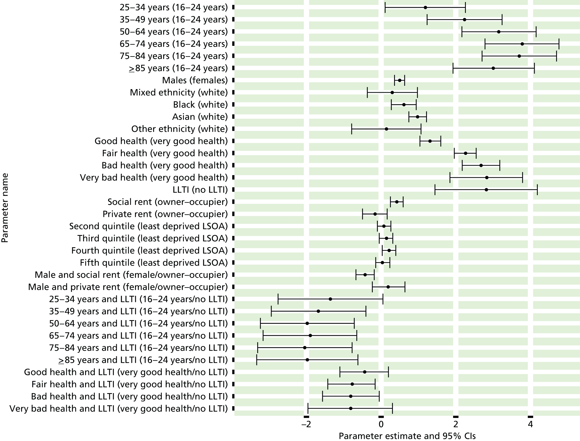
It is important to recognise that no direct causal relationship (or direction) is being claimed. The proposed model ‘merely’ offers the best means of utilising data (available for local areas) for predicting whether or not an individual will exhibit or develop a particular disease, condition or health-risk behaviour. To that extent, it does not matter, for instance, that it is having diabetes that, in causal terms, means that an individual is more likely to have a LLTI. From a predictive perspective, when one is able to use only data available for local areas, if an individual has a LLTI then this increases the likelihood that they will have diabetes – as it does, of course, across many of the other CVD/CVD-related and mental health problems considered in this study. At an individual level this is of limited utility, but when likelihood estimates (derived using all available sociodemographic data) are applied to populations, this allows us to predict how many adults are likely to have diabetes, or any of the other conditions in which we are interested.
The only complication when interpreting this, and most other parameter plots, is allowing for the possible impact of interaction effects. In this instance, although there is much uncertainty as to the exact scale of the effect, various combinations of age and LLTI, and of general health and LLTI, are included as having a statistically significant relationship with the likelihood that an individual will report diabetes as a LLTI. The complication is that these interact with the respective main effects, although in this instance the overall picture remains quite clear.
One final aspect of model fitting needs to be noted. All the surveys which provided data to this study utilised a stratified random probability sample to select households. This approach incorporates a geographic ‘primary sampling unit’ (PSU) in the sampling framework which, in theory, could result in some covariance. To test whether or not PSU membership explains any of the variation in each response variable, we fitted a ‘mixed’ model equivalent to the final generalised linear model. This generalised linear mixed model, implemented in R Statistics using the glmer function of the lme4 package,471 incorporated the PSU as a random effect and the size of that effect was considered. This was invariably statistically insignificant and could be discounted.
From parameter estimates to disease likelihoods
An exploration of the various tables and plots in Appendices 26 and 27 will illustrate the nature of the relationships which underpin the estimation of local disease prevalence rates, but it should be reiterated that these are essentially ‘predictive’ rather than ‘explanatory’ models. Indeed, in a very real sense it is quite unimportant whether or not the particular phenomena represented in the final models are, in themselves, causally related to morbidity. Rather, they represent the best fitted solution for predicting variations in morbidity using only variables for which cognate census-derived covariate data are also available. The issue is now how best to utilise the information captured by the survey-based models for predicting disease prevalence in small populations.
As outlined in the introduction to this chapter, the approach adopted is to use the parameter estimates to calculate the likelihood that different types of person, as defined by each model, will have a particular condition or disease. Thus, the model for ‘diabetes as a LSI illustrated by Figure 1 comprises six individual-level variables and a total of 24 factors: age band with seven factors (16–24 years, 25–34 years, 35–49 years, 50–64 years, 65–74 years, 75–84 years and ≥ 85 years); sex with two factors (male and female); ethnicity with five factors (white, mixed, black, Asian and other); general health status with five factors (very good, good, fair, bad and very bad health); LLTI with two factors (yes and no); and tenure with three factors (owner–occupier, social renting and private renting/other). This, in fact, defines 7 × 2 × 5 × 5 × 2 × 3 = 2100 ‘person-types’ for whom a specific disease likelihood can be calculated; this rises to 10,500 person types once one includes reference to the IMD quintile of the LSOA in which an individual lives. Different models will generate likelihood estimates for a different number of person-types depending on the number of factors in the model, but in all cases a rich description of how disease likelihood varies across the sociodemographic spectrum is provided. The particular advantage of this approach is that, in association with the use of interaction effects, the full compositional diversity of different populations can be incorporated into the final estimates of disease prevalence.
Microsimulation for small-area estimation describes how suitable local covariate data are obtained, and Small-area estimation: prediction describes how the person-type disease likelihood estimates are attached to those covariate data to finally derive the required local prevalence estimates, but a key difficulty with this process is how to incorporate parameter uncertainty into those prevalence estimates. Figure 1 makes clear that, even for clearly statistically significant parameters such as age, there is still considerable uncertainty around the actual parameter estimate.
Capturing uncertainty: a bootstrapping approach
Although this study commenced with the intention of using an explicitly Bayesian approach, in practice this proved problematic, principally because of the computational demands of Markov chain Monte Carlo which, in the context of fitting multiple models with many parameters and with respect to relatively large data sets, proved too time-consuming. The perceived advantage of a Bayesian approach had been that, in explicitly generating posterior distributions for small-area estimates, it offered a suitable framework for capturing model uncertainty in the final estimates. Retaining this focus on understanding estimate uncertainty was deemed essential, and thus we turned to an alternative method of inferring the precision of the estimates based on a well-established technique known as bootstrapping.
The classic illustration of bootstrapping concerns estimating the mean height of people worldwide. We cannot measure the heights of all people in the global population, so instead we sample only a tiny part of the population and measure the height of the people within that. From this sample of n individuals a single mean height is obtained, but we have no sense of how reliable that mean estimate actually is. The bootstrap approach involves multiple resampling (with replacement) from the original sample to obtain a large number of bootstrap samples, from each of which we derive a mean height. From this set of ‘bootstrapped’ means we can calculate both an overall ‘point estimate’ and 2.5% and 97.5% quantiles to indicate the range over which we are 95% confident that the actual global mean lies (assuming, of course, that we had taken a suitably representative sample in the first place).
The key feature of the bootstrap approach as applied here is that, following standard practice, multiple bootstrap (‘with replacement’) samples were taken of the original survey data set (retaining the PSU structure to reflect the underlying sampling methodology) and each was then used to generate a new set of model parameter estimates. Given the time available, 220 bootstrap samples, and, thus, 220 independent sets of parameter estimates, were obtained for each model. This is a very small number compared with most bootstrap procedures (which typically extract thousands of samples) and the precision of the upper and lower 95% CIs will be affected, but it is worth emphasising that each bootstrap sample is used to generate 220 sets of likelihood estimates for each and every one of the 10,500 person-types, and that these are then aggregated to generate the 220 sets of estimates for all LSOAs, MSOAs and higher geographies. Although this massively increases the computational burden, it enables us to extract summary statistics to capture how model-based uncertainty affects the final estimates at all scales. Thus, as detailed in Small-area estimation: prediction, the range within which 95% of the 220 bootstrap-based estimates lie provides a good, albeit approximate, empirical measure of the 95% credible interval. (The term ‘credible interval’, rather than ‘confidence interval’, is preferred, as it represents a region, sometimes known as the ‘credible region’, of the predictive distribution defined by the 0.025 and 0.975 quantiles.)
Microsimulation for small-area estimation
As noted above, a ‘bottom-up’ approach to small-area estimation requires that the disease ‘likelihood estimates’ calculated for each of the individual ‘person-types’ defined at the modelling stage can be applied to appropriate counts of the number of such ‘person-types’ in each LSOA. The principle is straightforward: if there is a 0.2 risk that a particular type of person (defined in terms of age, sex, general health and whatever other variables are included in the model) has a particular disease, and there are 10 such people in a particular LSOA, then 2 of the 10 people in the LSOA might be expected to have the disease. Summing the results of this calculation across all ‘person-types’ provides an estimate of the total number of people in the LSOA with the disease, and dividing by the relevant population denominator provides the required prevalence rate. The implementation of this algorithmic process is described in Small-area estimation: prediction, but it fundamentally depends on being able to fully describe the composition of the relevant population; not just in terms of a series of cross-tabulations available for 2011 census data, but in terms of the number of people in each uniquely defined person-type category. In other words, to take a trivial example, rather than knowing how many males and females there are in a particular area and, separately, how many people report having ‘very good’, ‘good’, ‘fair’, ‘bad’ and ‘very bad’ health, we now need to know how many males have very good health, how many females have very good health, and so on. In general terms, we need to utilise the information available in existing census tables on the aggregate characteristics of LSOA populations (so-called ‘marginal distributions’) to derive an estimate of the underlying, and unknown, ‘full joint distribution’.
An approach generically known as ‘iterative proportional fitting’ has long been used to combine marginal distributions (including two-, three- and four-way joint distributions) to derive full joint distributions. Such approaches are often constrained to a dependency structure derived from an analysis of individual-level sample data, such as is provided for the 2001 census data by the Individual Sample of Anonymised Records. Unfortunately, when the analysis was undertaken, sample-based micro data were not yet available for the 2011 census and, as a result, our implementation iterative proportional fitting cannot utilise such information.
We have thus developed a form of iterative proportional fitting which seeks to iteratively assign individuals to cells in the full joint distribution in such a way as to minimise a test statistic which sums the aggregate difference between the resulting ‘provisional’ marginal estimates and the ‘known’ marginal totals taken from the census tables listed in Table 4. At each iteration, individuals are moved between cells to minimise the test statistic until, in theory, an allocative solution is found in which the full joint distribution matches in all respects what is known, through the census-based marginal totals, about a population.
At the heart of this approach is a (0,1) relational matrix linking each person-type with each of the ‘known’ marginal totals. Table 9 provides a (highly) simplified illustration of how this matrix allows the estimated number of people in each marginal total (the right-hand column) to be related to the known marginal totals (the penultimate row). This example assumes there to be three census tables through which we know there are 51 males and 49 females; 75 people aged 16–54 years and 25 people aged 55–74 years; and 53 people with a LLTI and 47 people without. Although the tables tell us nothing about the full distribution, by iteratively moving individuals between person-types (using a constrained ‘random walk’) we can calculate, as given in the final row of the table, how close the estimated number of people in each person-type category is to a fitted solution. The goal, of course, is to determine an allocation which results in a set of estimated marginal totals that equals, or very closely approximates, the set of known marginal totals. In this case a ‘fitted’ solution would be achieved (i.e. with all column ‘absolute differences’ = 0) using the person-type counts given in brackets.
| Person-type category | Link matrix | Estimated number of people in category | |||||
|---|---|---|---|---|---|---|---|
| M | F | 16–54 years | 55–74 years | LLTI | No LLTI | ||
| M, 16–54 years, LLTI | 1 | 0 | 1 | 0 | 1 | 0 | ←27 (26) |
| M, 16–54 years, no LLTI | 1 | 0 | 1 | 0 | 0 | 1 | ←14 (15) |
| M, 55–74 years, LLTI | 1 | 0 | 0 | 1 | 1 | 0 | ←7 (5) |
| M, 55–74 years, no LLTI | 1 | 0 | 0 | 1 | 0 | 1 | ←5 (5) |
| F, 16–54 years, LLTI | 0 | 1 | 1 | 0 | 1 | 0 | ←14 (16) |
| F, 16–54 years, no LLTI | 0 | 1 | 1 | 0 | 0 | 1 | ←16 (18) |
| F, 55–74 years, LLTI | 0 | 1 | 0 | 1 | 1 | 0 | ←8 (6) |
| F, 55–74 years, no LLTI | 0 | 1 | 0 | 1 | 0 | 1 | ←9 (9) |
| Estimated marginal count of persons | ↓ | ↓ | ↓ | ↓ | ↓ | ↓ | |
| 53 | 47 | 71 | 29 | 56 | 44 | Sum of absolute differences | |
| Known marginal count | 51 | 49 | 75 | 25 | 53 | 47 | |
| Absolute difference | 2 | 2 | 4 | 4 | 3 | 3 | →18 |
In reality the process is significantly more complex, involving a link matrix with 21,000 ‘person-type’ rows [covering the 10,500 person types described above living in (a) households and (b) communal establishments] and 384 ‘marginal total’ columns (relating to census table marginal totals). The iterative process was extremely computationally demanding, not least because it had to be replicated for each of the 32,844 LSOAs for which prevalence estimates were to be produced. It was eventually scripted using a new high-level, high-performance dynamic programming language for technical computing known as Julia472 and, in practice, we allowed the iteration to terminate when the sum of absolute differences (across all 384 columns) fell below five. The length of time it took to achieve a perfect solution could not be justified given that the original census data had been perturbed to ensure confidentiality.
The key point is that any final ‘fitted’ solution constitutes a detailed description of the composition of an area which matches, or almost matches, what is known (through available census tables) about an LSOA. We can then apply modelled likelihood estimates for each ‘person-type’ to appropriate count data. This, we believe, greatly increases the specificity of the final estimates, particularly with respect to the way in which parameter interaction effects will play out in different areas. It is, however, important to recognise that multiple solutions (at least in theory) will exist to any given set of marginal totals. This implies additional uncertainty to the final estimates which have not been fully investigated and which are not captured by the formal estimate CIs.
Small-area estimation: prediction
The prediction component of small-area estimation is an entirely straightforward and algorithmic process, even though it raises, once again, substantial computational challenges. Modelling large-scale surveys described how appropriate models were specified and fitted to large scale-survey data with a view to producing up to 10,500 person-type specific disease ‘likelihood’ estimates for each of the 65 response items considered. It also described how bootstrapping was, in each case, used to generate 220 independent estimates which captured model parameter uncertainty. Microsimulation for small-area estimation, meanwhile, described how available multivariate census tables were used to ‘microsimulate’ a full joint distribution for each LSOA which, in effect, provides a description of the detailed sociodemographic composition of each LSOA. Now the task is ‘simply’ one of applying the appropriate disease likelihood risks to the relevant counts of the number of people in each person-type category in each LSOA, and then summing the products to determine how many people in each LSOA (and higher unit) are likely to have the disease.
Here, the issue is how, precisely, should those disease risk likelihood estimates be applied? The fact of the matter is that a particular individual will either have a disease or not have a disease. They will not have 0.2 of a disease, even if that is the underlying probability. As simply summing the probabilities of illness multiplied by the number of individuals to which they applied would underestimate the uncertainty implicit in the likelihood estimates, a more appropriate approach is to predict for each individual in the population (on the basis of their individual disease likelihood) whether or not they have the disease/condition in question, and then sum these predictions. This, of course, is a Bernoulli trial, and now the overall prevalence rate is not simply the sum of ‘likelihoods × counts’, but rather the sum of the outcomes of Bernoulli ‘coin tosses’ applied to each and every individual in the population.
In this way, we capture not only model uncertainty by replicating the process for each of the 220 bootstrapped data sets – resulting in 220 independent sets of parameter estimates which are used to compute 220 independent disease risk estimates for each of the 10,500 person-types – but also the inherent uncertainty concerning whether or not an individual, with a particular risk, will have the disease. The outcomes of the Bernoulli trials are then summed for 12 age-/sex-defined cohorts, and for the overall population, in each LSOA and all higher units. This results, in each case, in 220 bootstrap-based estimates of the number of people we predict will have the disease or condition in question. The final step, therefore, is to describe the resulting distributions in terms of the range within which 95% of the values fall. These summary data are then retained and constitute the information to be made available via PHE’s local health website. 441
To clarify, therefore, the MSOA, LA, CCG and all other estimates have not been generated by statistically amalgamating LSOA-level summary estimates, but by directly undertaking Bernoulli trials, based on appropriate disease risk likelihoods, with respect to all individuals within the units in question. It is worth noting that smaller credible intervals (explicitly the range within which 95% of the 220 bootstrapped estimates fall) are obtained for larger populations purely because variability induced by bootstrapping and the Bernoulli trial is dampened. Underlying model uncertainty remains the same throughout, resulting in a less dramatic improvement in estimate precision than might have been expected.
Chapter 4 Investigating equity in the utilisation of cardiovascular services
Introduction
The aim of this chapter is to determine the extent to which variations in the presentation and management of CVD reflect underlying differences in the health-care needs of populations. To this end, we have rejected the use of administrative data to proxy need (as this, we argue, runs the risk of reflecting both unmet need and unjustified supply) and have instead developed modelled estimates of cardiovascular need. The methods used to this end were described in Chapter 3. In this chapter we (a) test the estimates and select which, of a number of various indicators, we will use in our investigation of use relative to need, and (b) investigate the extent to which PCT- and practice-level variations in the presentation, primary management and specialist management of diabetes, CHD, hypertension and stroke can be explained by underlying need and/or population characteristics (deprivation, age, ethnicity and rurality).
The importance of capturing health-care needs
As discussed in Chapter 2 (see Methodological issues and Administrative data), one approach to exploring issues of equity has been to use administrative data as denominators of need. 205,213,291,295,299–301,305,306,311 Here, ‘prevalence rates’ refer to, for example, QOF ‘prevalence’ rates (the number of people on GP registers for particular conditions such as depression, CHD or hypertension) or the proportion of hospital patients admitted with a particular diagnosis (such as angina). This can throw light on variations in access and use once patients are ‘within’ the health service, for example the extent to which particular treatments and/or procedures are provided relative to the number of people admitted with a particular diagnosis. It does not, however, address the extent to which different populations and cohorts use health services relative to the underlying prevalence of illness because expressed demand inevitably incorporates both unmet need and unjustified supply.
Primary care trust- and CCG-level modelled disease prevalence rates disseminated by the Public Health Observatories and, more latterly, PHE, try to get around this problem by modelling direct estimates of disease prevalence within the community. 210–215,473 These have not, however, been widely used in studies of health service equity211,215,222,474–476 and, as discussed below, there are some questions regarding their relative reliability for underpinning studies of health service equity.
Ignoring access to and use of health services relative to underlying needs is a problem in its own right as it leaves unexplored a key aspect of access, but it has a broader significance insofar as variations in rates of specific treatments and/or procedures within the health service must, to some degree, reflect variations in initial presentation. This is not simply because, at an individual level, belated presentation is likely to result in the need for higher levels of health care at a later date. Even allowing for this, if a smaller proportion of any given population is presenting with early and/or minor symptoms, this will tend to ‘weight’ the cohort and make it appear that, relative to the number of people who have actually presented, a higher level of care is being provided. The potential contradiction is obvious, and there is a real danger that one is not comparing like-with-like denominator populations when examining ‘within-system’ variations. The point is that it is difficult to adequately interpret ‘within-system’ variations in the use of particular treatments without reliable evidence on underlying needs in the broader community.
Estimating the prevalence of particular diseases and conditions in the community is thus key to any full understanding of health-care equity, as well as, of course, of potential significance for public health planning and the commissioning of services. Developing a robust approach for generating prevalence estimates for small populations and, more specifically, redressing the effective absence of such data for key cardiovascular and mental health conditions has been a core project objective. To that end a range of prevalence estimates have been produced. The problem, though, is how can one assess the reliability of those prevalence estimates as a baseline for studies of equity of use of specific health services?
Cardiovascular disease prevalence estimates: testing for reliability
The lack of a gold standard
The fact of the matter is that there is no ‘gold standard’ measure of disease prevalence against which to assess the prevalence estimates. Indeed, if there were, those estimates would immediately become redundant. Legitimacy can only flow from methodological rigour (the subject of the previous chapter) and, problematically, a somewhat circular comparison with available utilisation data. This is circular (and problematic) in the sense that, although the prevalence rates are to be used as a measure of underlying illness (need) in an assessment of how health service use varies relative to need, the only evidence we have on variations in illness lies with data collected by the NHS about people who have actually accessed some form of health care. This is not optimal, but it is inescapable.
The fundamental problem is, thus, that it is impossible to prove whether or not discrepancies, whether systematic or stochastic, are due to inadequacies in the need estimates or because of variations in uptake relative to need. However, although definitive proof may be elusive, we would argue that confidence in the legitimacy and usefulness of the prevalence estimates generated can be obtained by comparing them in detail against a variety of measures of health service utilisation. We acknowledge that, for any particular scenario, contradictory interpretations can always be placed on the same observations – discrepancies between need estimates and utilisation data could be due to inadequacies in the needs estimates or because of local variations in access – but it is the overall weight of evidence in the context of a coherent explanatory narrative that matters.
Quality and Outcomes Framework data
In this section, therefore, we compare our CVD need estimates with QOF disease registration data. The QOF database72,440 publishes counts of people on each practice disease register and, using denominators based on overall or age-specific patient populations, practice-level prevalence rates. As practices are paid for keeping the registers, and as the number of people on their disease registers is used to calculate payments within each of the clinical indicator groups, the policy intention is that registers are properly kept and that efforts are made to ensure that as many patients as possible with the specified conditions are identified and registered. As a result QOF-based prevalence rates have been used as a source of proxy data on the level of health-care need in different populations. 140,243,247,259,262,289,477
There are, however, significant problems with the use of QOF disease registers, both generally and as a comparator against which to assess the reliability of our model-based need estimates. The first is their provenance as a tool designed to influence and reward GP behaviour. This can have very specific implications, such as the fact that an individual can be included on the diabetes register only if the practice has established not only that a patient has diabetes, but whether the diabetes is type 1 or type 2. A more fundamental problem is that QOF prevalence rates will reflect variations in case finding. One consequence is that they tend to increase over time (inclusion of registers within the QOF payments system was, in part, intended to improve case finding). More significantly, case finding will also vary in response to factors such as the time, commitment and resource GPs direct towards such activity as well as, no doubt, the responsiveness of the populations being served.
A further issue is the fact that no information is available on the age–sex profile of patients included on the various QOF disease registers. 478 The published QOF prevalence rates are ‘crude’ rates affected by differences in, or changes to, the demographic composition of practice populations. Practices, PCTs and CCGs have very different populations and variations in ‘crude’ QOF prevalence rates are as likely to reflect varying demographic structures as any genuine difference in the health status of populations. Indeed, the stronger a disease’s demographic gradient, the more problematic will be the QOF prevalence rate.
Such problems notwithstanding, the QOF registers explicitly count the number of people ‘known’ by GPs to have a series of specific conditions and, as such, represent a key measure of primary presentation. We can thus simultaneously ‘test’ our estimates by assessing whether or not they broadly align with the number presenting and, by focusing on the differences between presentation (QOF registration) and underlying need (modelled prevalence estimates), can begin to investigate the nature and scale of variations in the utilisation of primary care.
Determining appropriate need indicators
Although we are principally concerned (as detailed below) with comparing how counts and rates vary at more local levels (practices, PCTs and CCGs), we must first establish which of the modelled prevalence rates are likely to provide the most reliable guide to variations in the underlying prevalence of the conditions for which suitable QOF data are available, namely diabetes, CHD, hypertension, stroke and, in Chapter 5, depression. As argued in Chapter 3 (see Methodology overview), it was not possible to determine a priori which of the prevalence rates that could be derived from large-scale survey data would provide the most ‘useful’ indicators of health-care needs. Thus, a range of alternative prevalence rates have been modelled – distinguished by definitional differences and/or because they have been drawn from different surveys using different predictor variables. This is of particular relevance to depression (see Chapter 5, Variations in the use of mental health services relative to need), where a large and very diverse range of prevalence rates is available and where there is scant a priori evidence on which to choose between them.
The only sensible approach to deciding between the alternative prevalence rates as potential indicators of ‘health service needs’ is to incorporate an assessment of how well they compare with the QOF registration data. This is not the only consideration, for there are often definitional differences that affect how the estimates should be interpreted (such as the distinction between biometric, diagnosis-based and self-reported LSI measures), but it is nonetheless important that a convincing explanatory narrative can link any putative measure of ‘health service need’ with the only proxy source we have on the number of people known to have such a need, namely the number of people on QOF registers.
Diabetes
Although diabetes is not classed as a ‘cardiovascular disease’, colleagues at PHE encouraged us to generate diabetes prevalence estimates as diabetes is of key interest to the public health community. Furthermore, key aspects of the disease make it a useful benchmark condition against which to compare modelled and QOF prevalence rates. First, diabetes is a well-recognised condition and individuals responding to the HSfE are likely to be using the term in a way that is directly and unequivocally comparable with its use in the QOF. Prescribing and inpatient utilisation data relating to diabetes are relatively unambiguous (unlike a number of CVD drugs that can be prescribed for a range of clinical conditions). The QOF diabetes register also refers to an age-defined cohort (albeit of patients aged 17 years or older, whereas our modelled estimates relate to people aged 16 years or older).
As Table 10 shows, the overall number of patients estimated to have diabetes in the community (however defined) is very similar to the overall number of people on the QOF register. This implies relatively good case-finding in primary care settings although, as might be expected, the number of people estimated to have ‘doctor diagnosed or undiagnosed diabetes’ slightly exceeds the number who have been diagnosed with diabetes, who report diabetes as a LSI, or who appear on the QOF register.
| QOF register | Practice population (≥ 17 years) | Patients (≥ 17 years) on register | QOF prevalence rate, % |
|---|---|---|---|
| Diabetes mellitus 2010–11 | 44,291,915 | 2,455,937 | 5.5 |
| Diabetes mellitus 2011–12 | 44,569,825 | 2,566,436 | 5.8 |
| Potential diabetes needs indicators (2001 ADS population ≥ 16 years = 44,813,241) | |||
| Modelled prevalence | Predicted cases (≥ 16 years) | Prevalence rate, % (95% CI) | |
| As a LSI | 2,118,013 | 4.7 (4.4 to 5.0) | |
| Doctor diagnosed | 2,577,799 | 5.2 (4.6 to 5.8) | |
| Diagnosed and undiagnosed | 2,900,779 | 6.5 (5.9 to 7.0) | |
The crucial question, though, is the extent to which each of these potential needs indicators correlates with QOF registrations at practice and PCT level. We consider below how use-to-need rates vary at practice and PCT level with respect to a range of health service activities, but here we examine how estimated counts of the underlying number of people with diabetes in practices and PCTs compare with counts of the number of people on the QOF diabetes disease register. Correlation statistics for count data can mislead because of the overwhelming effect of population size on the number of people with any given condition, but this nevertheless avoids any potential bias arising from different demographic profiles. If the modelled estimates are accurate, and are thus a useful guide to variations in the need for services, they should be highly predictive of the number of people who are QOF registered.
Alongside overall QOF and modelled estimate prevalence rates, Table 11 records PCT-level ratios of QOF and modelled prevalence with respect to each of the potential definitions of needs. For instance, in terms of the need indicator based on the number of people estimated to have diabetes as a LSI, there is a 1.77-fold variation in PCT-level registrations per expected (modelled) case (from 0.91 registrations per case and 1.77 registrations per case). Table 11 also reports the extent to which the QOF registration counts are correlated with the various estimates of the number of people with diabetes. Thus, 97.5% of the variation in QOF registrations can be explained by the need indicator based on the LSI indicator. This is a somewhat larger proportion than either of the alternatives, based on ‘doctor-diagnosed diabetes’ and a composite measure of ‘diagnosed and undiagnosed diabetes’, which explain 95.9% and 96.8% of the variation in QOF registration counts, respectively. All three definitions of need generate estimates that are much better at predicting QOF registrations than the size of the underlying ‘at-risk’ populations, which accounts for ‘just’ 93.5% of PCT-level variation. This is also true at practice level (n = 8067), with the ‘LSI’ indicator explaining 90.8% of the variation in practice-level QOF registration counts, compared with just 75.9% explained by the size of the ‘at-risk’ population.
| Denominator population | Prevalence rate (%) | Registrations per expected case | Count correlation | |||
|---|---|---|---|---|---|---|
| Mean | Minimum–maximum | Variation | R | % R2 | ||
| Total QOF population (≥ 17 years) | 5.8 | – | – | – | 0.967 | 93.5 |
| Adults reporting diabetes as a LSI | 4.7 | 1.20 | 0.91–1.61 | 1.77 | 0.988 | 97.5 |
| Adults ever been doctor-diagnosed with diabetes | 5.2 | 1.08 | 0.85–1.84 | 2.16 | 0.979 | 95.9 |
| Adults with diagnosed or undiagnosed | 6.5 | 0.88 | 0.63–1.12 | 1.78 | 0.984 | 96.8 |
It is perhaps surprising that the estimates based on LSI should prove more effective at predicting variations in QOF registrations than either of the alternatives, which, after all, incorporate information on actual diagnosis. This may be attributable to the fact that many more survey responses are available with respect to ‘diabetes as a LSI’ (n = 29,905) than to either ‘doctor-diagnosed diabetes’ (n = 18,684) or ‘diagnosed and undiagnosed diabetes’ (n = 11,061). As a direct result, LSI -based estimates are more precise (as detailed in Appendix 26) and the relationship with the phenomenon being described less subject to less uncertainty.
Choosing which prevalence rate best proxies needs is a balance between definitional, evidential and predictive considerations. ‘Diabetes as a LSI’ is perhaps a less satisfactory definition of underlying morbidity than one which includes a biometric assessment of clinical diabetes (e.g. ‘diagnosed and undiagnosed diabetes’), and it does give rise to estimates that are somewhat lower than indicated by QOF registrations (4.7% as opposed to 5.8%). However, in this case the extent to which it predicts variations in QOF registrations suggests that it offers the most appropriate ‘needs indicator’ for our analysis of the factors which influence variations in QOF registration, prescribing and inpatient activity. Such interpretative issues affect decisions about all of the modelled prevalence estimates. In order to make these as transparent as possible, information about the definition, provenance and prediction of modelled variables is provided in Appendix 26.
Coronary heart disease
Once again a number of modelled prevalence rates are available as potential ‘needs indicators’ for CHD. These are based on the following definitions:
-
‘CHD as a LSI’ – explicitly including ‘heart attack’, ‘angina’, ‘coronary thrombosis’ and ‘MI’; the only difficulty here is that coding is of respondent descriptions and this may not always be clinically precise enough to categorise as CHD.
-
‘Doctor-diagnosed CHD’ – respondents stating that a health professional had diagnosed ‘angina or a heart attack (including MI and coronary thrombosis)’.
-
‘CHD symptoms (angina and/or MI)’ – respondents reporting that they have ever had chest pain in sternum, sternum lower or anterior lower chest and in the left arm (possible angina) or have had severe pain across the front of their chest lasting half an hour or longer (possible MI).
-
‘Clinical evidence of CHD’ – respondents who have ever had symptoms of angina and/or MI (as above), who are currently taking drugs for CHD (see Appendix 26 for details), or who have recently (past 12 months) been diagnosed with angina or having had a heart attack.
-
‘Current evidence of CHD’ – extends the ‘clinical evidence’ definition to include respondents who self-report angina and/or heart attack as a LSI.
-
History of CHD’ – extends the ‘current evidence’ definition to include respondents who have ever been diagnosed with angina or having had a heart attack (rather than being restricted to those diagnosed in the past 12 months).
As shown in Table 12, national prevalence rates (for adults aged ≥ 16 years) based on these definitions range from 2.0% to 12.5% as opposed to the national QOF CHD prevalence rate of 3.4% (for people of all ages).
| QOF register (all ages) | Practice population (all ages) | Patients on the register | QOF prevalence rate, % |
|---|---|---|---|
| CHD 2010–11 | 55,169,643 | 1,877,518 | 3.4 |
| CHD 2011–12 | 55,525,732 | 1,875,548 | 3.4 |
| Potential CHD needs indicators (2001 ADS population ≥ 16 years = 44,813,241) | |||
| Modelled prevalence | Predicted cases (≥ 16 years) | Prevalence rate, % (95% CI) | |
| As a LSI | 909,846 | 2.0 (1.9 to 2.2) | |
| Doctor-diagnosed CHD | 2,406,474 | 5.4 (4.9 to 5.8) | |
| CHD symptoms (angina/MI) | 3,769,658 | 8.4 (7.8 to 9.0) | |
| Clinical evidence of CHD | 5,213,527 | 11.6 (10.9 to 12.4) | |
| Current evidence of CHD | 5,294,388 | 11.8 (11.1 to 12.5) | |
| History of CHD | 5,616,107 | 12.5 (11.8 to 13.3) | |
As with diabetes, the modelled estimate of the number of people living with CHD as a long-standing disease is somewhat lower than the number of patients on the QOF disease register. In both cases this probably reflects the way respondents to the HSfE respond to a question that asks them to record as a LSI anything that ‘has troubled you over a period of time, or that is likely to affect you over a period of time’. For some, a well-controlled condition may not be seen as ‘troubling’, though a GP should still place them on the CHD register. This would also explain why a substantial proportion of people who report having been diagnosed with CHD fail to report it as a LSI.
The 3.4% QOF prevalence rate for people of all ages equates, in broad terms, to a rate of about 4.2% for adults aged 16 years or older. It is interesting that this falls short of the proportion of people estimated to have been doctor diagnosed (5.4%), though this may simply be due to this estimate being based on a lifetime recall of ever having had the disease compared with the people being entered onto the register since it was implemented in 2004–5.
The QOF rate also falls short of the proportion of people expected to have CHD symptoms, and a long way short of the remaining measures. This tallies with previous research comparing modelled APHO CHD prevalence and diagnosed prevalence215 and is indicative of significant levels of undiagnosed and unrecognised CHD in the community. In Chapter 5 (see Common mental health disorder prevalence estimates: testing for reliability) we examine whether or not there is any evidence of systematic variations in unmet need, but it is again first necessary to determine which of the prevalence rates is likely to provide the most useful measure of health service needs.
Following the approach described with respect to diabetes, and referring to the information summarised on Table 13, in this case it is ‘doctor-diagnosed’ CHD which most closely predicts PCT-level variations in QOF registrations (% R2 = 97.4%). This is, of course, exactly what one should expect given that the definitions are precisely cognate. It would, however, obviously be problematic to use such an explicitly utilisation-based measure of needs as the basis for assessing how use varies relative to needs. A case could again be made for using the LSI definition as a proxy needs indicator, as this exhibits the least variation in registrations per expected case and, after ‘doctor diagnosis’, best explains variations in the overall number of registrations at PCT level. In this case, however, the overall prevalence rate falls so far short of the QOF registration rate that it seems more appropriate to use ‘clinical evidence of CHD’ as the basis on which to measure health service needs. This captures whether people have ever had symptoms of angina or MI, are taking prescribed drugs for CHD, or have recently been diagnosed with angina or having had a heart attack.
| Denominator population | Prevalence rate, % | Registrations per expected case | Count correlation | |||
|---|---|---|---|---|---|---|
| Mean | Minimum–maximum | Variation | R | % R2 | ||
| Total QOF population (all ages) | 3.4 | – | – | – | 0.918 | 84.3 |
| Total population ≥ 16 years | 4.2 | – | – | – | 0.924 | 85.4 |
| Adults reporting CHD as a LSI | 2.0 | 2.02 | 1.32–2.54 | 1.92 | 0.980 | 96.0 |
| Adults ever been doctor diagnosed with CHD | 5.4 | 0.78 | 0.48–0.97 | 2.02 | 0.987 | 97.4 |
| Adults with angina/MI symptoms | 8.4 | 0.49 | 0.24–0.66 | 2.75 | 0.966 | 93.4 |
| Adults with clinical evidence of CHD | 11.6 | 0.35 | 0.19–0.45 | 2.37 | 0.978 | 95.6 |
| Adults with current evidence of CHD | 11.8 | 0.35 | 0.19–0.44 | 2.32 | 0.979 | 95.8 |
| Adults with any history of CHD | 12.5 | 0.33 | 0.18–0.42 | 2.33 | 0.979 | 95.9 |
The ‘clinical evidence of CHD’-based definition explains 95.6% of the variation in PCT-level QOF registrations, considerably more than the 85.4% explained simply with respect to the number of people aged 16 years or older. The ‘clinical evidence’ definition of CHD prevalence also explains far more of the variation in QOF counts at practice level (n = 8068), in this case 90.4% compared with the 68.7% that can be explained with reference to the number of ‘at-risk’ people in each practice.
Hypertension (high blood pressure)
High blood pressure is also a well-defined and widely recognised condition which respondents to the HSfE might be expected to report reliably, although it should be noted that the QOF threshold for high blood pressure is 150/90 mmHg, compared with the 140/90 mmHg threshold used in the HSfE. Also blurring precise comparability is the fact that clinical hypertension requires elevated readings to be obtained on more than one occasion, whereas the survey-based designation of high blood pressure is based on a one-off reading.
Once again, as illustrated in Table 14, considerably fewer people report high blood pressure as a LSI than appear in the QOF hypertension disease register, presumably for the same reasons as given above. What is most notable, however, is the very much higher number of people estimated to have high blood pressure when that estimate is derived from variables relating to nurse measurement or diagnosis. Here, the alternative estimates are based on:
-
‘nurse-measured high blood pressure’ – the number of survey respondents with a systolic reading of > 140 mmHg and/or a diastolic reading of > 90 mmHg
-
‘nurse-measured high blood pressure or blood pressure drugs’ – which extends the definition to include respondents taking diuretics, beta-blockers, ACE inhibitors, calcium channel blockers or ‘other blood medication’ specifically intended to control high blood pressure
-
‘clinical evidence of high blood pressure’ – which further incorporates respondents diagnosed with current high blood pressure
-
‘any evidence of high blood pressure’ – which finally includes respondents who have ever been diagnosed with high blood pressure or who report it as a LSI.
| QOF register | Practice population (all ages) | Patients on the register | QOF prevalence rate, % |
|---|---|---|---|
| Hypertension 2010–11 | 55,169,643 | 7,460,497 | 13.5 |
| Hypertension 2011–12 | 55,525,732 | 7,567,965 | 13.6 |
| Potential hypertension needs indicators (2001 ADS population ≥ 16 years = 44,813,241) | |||
| Modelled prevalence | Predicted cases (≥ 16 years) | Prevalence rate, % (95% CI) | |
| As a LSI | 3,010,018 | 6.7 (6.5 to 7.0) | |
| Nurse-measured | 9,251,361 | 21.5 (20.2 to 21.5) | |
| Nurse-measured or on blood pressure drugs | 13,408,487 | 30.1 (29.4 to 30.7) | |
| Clinical evidence | 14,473,610 | 32.5 (31.9 to 33.0) | |
| Any evidence | 16,101,059 | 36.1 (35.4 to 35.7) | |
These definitions may appear progressively inclusive, but it is important to recognise that they also differ in terms of potential utilisation and social bias and their interpretation is not entirely straightforward. For instance, although nurse-measured blood pressure data may seem free of bias – they are effectively based on blood pressure readings taken from a random sample of household residents – in fact a proportion of people will have normotensive blood pressure only because they are on medication. As an individual’s recognition that they need to seek treatment may not be socially neutral, and may furthermore reflect the availability and accessibility of appropriate health care, this measure would, somewhat perversely, tend to underestimate the needs of populations which are actually receiving high levels of support through prescribing and the associated primary management of hypertension. It would seem reasonable, therefore, to include people who report that they are currently taking prescription drugs to control blood pressure. But, if so, what about individuals who have been diagnosed with hypertension but who (possibly because of non-pharmacological treatments and/or lifestyle changes) do not provide a high blood pressure reading to the nurse administering the HSfE? They too have demonstrably made demands on health services (at the very least having been diagnosed by a health professional), even though to include them risks incorporating additional supply-side bias. Finally, what about those who return a normal blood pressure reading but who report high blood pressure as a LSI? There may be socioeconomic and/or demographic bias in how individuals respond to the LSI question, but, arguably, if a respondent states that a condition has ‘troubled’ them over a period of time, they have, by definition, a health-care need.
Given the possible sources of bias it is perhaps surprising that, as shown in Table 15, all of the definitions generate estimates that prove to be extremely powerful at predicting PCT-level QOF registration counts. From a public health perspective there may be a case for adopting the most inclusive ‘any evidence’ definition, but marginally the best predictor of variations in PCT-level registration is based on ‘clinical evidence’ of diagnosed or undiagnosed high blood pressure. This predicts a remarkable 99.2% of the variation in PCT-level QOF registrations. The advantage of using this prevalence rate as a ‘needs indicator’ for hypertension is illustrated effectively by Figure 2. This contrasts scatterplots of QOF registrations against (a) at-risk populations (people aged ≥ 16 years) and (b) the estimated number of people with hypertension. The former is relatively effective (predicting 94.3% of the variation in QOF registrations), but use of the ‘clinical evidence’-based measure of needs drags the outliers into an almost straight line. Using this indicator of needs has an equally dramatic impact with respect to practices (n = 8181), for which 77.8% of the variation in QOF registration counts can be explained by variations in the size of the underlying ‘at-risk’ practice populations, as opposed to 94.1% if one uses the number of people expected to have hypertension in each practice.
| Denominator population | Prevalence rate, % | Registrations per expected case | Count correlation | |||
|---|---|---|---|---|---|---|
| Mean | Minimum–maximum | Variation | R | % R2 | ||
| Total QOF population (all ages) | 13.6 | – | – | – | 0.971 | 94.3 |
| Total population ≥ 16 years | 16.9 | – | – | – | 0.974 | 94.9 |
| Adults reporting hypertension as a LSI | 6.7 | 2.50 | 1.99–2.88 | 1.45 | 0.994 | 98.8 |
| Adults with nurse-measured hypertension | 21.5 | 0.81 | 0.59–0.95 | 1.61 | 0.995 | 99.0 |
| Adults with nurse-measured or taking drugs for hypertension | 30.1 | 0.56 | 0.42–0.66 | 1.55 | 0.996 | 99.2 |
| Adults with clinical evidence of hypertension | 32.5 | 0.52 | 0.40–0.61 | 1.53 | 0.996 | 99.2 |
| Adults with any evidence of hypertension | 36.1 | 0.47 | 0.35–0.54 | 1.57 | 0.995 | 99.1 |
FIGURE 2.
Primary care trust-level QOF registrations against population and modelled estimate denominators: hypertension. (a) Population (≥ 16 years) against QOF registrations, 2011–12; and (b) estimate (≥ 16 years) against QOF registrations, 2011–12.
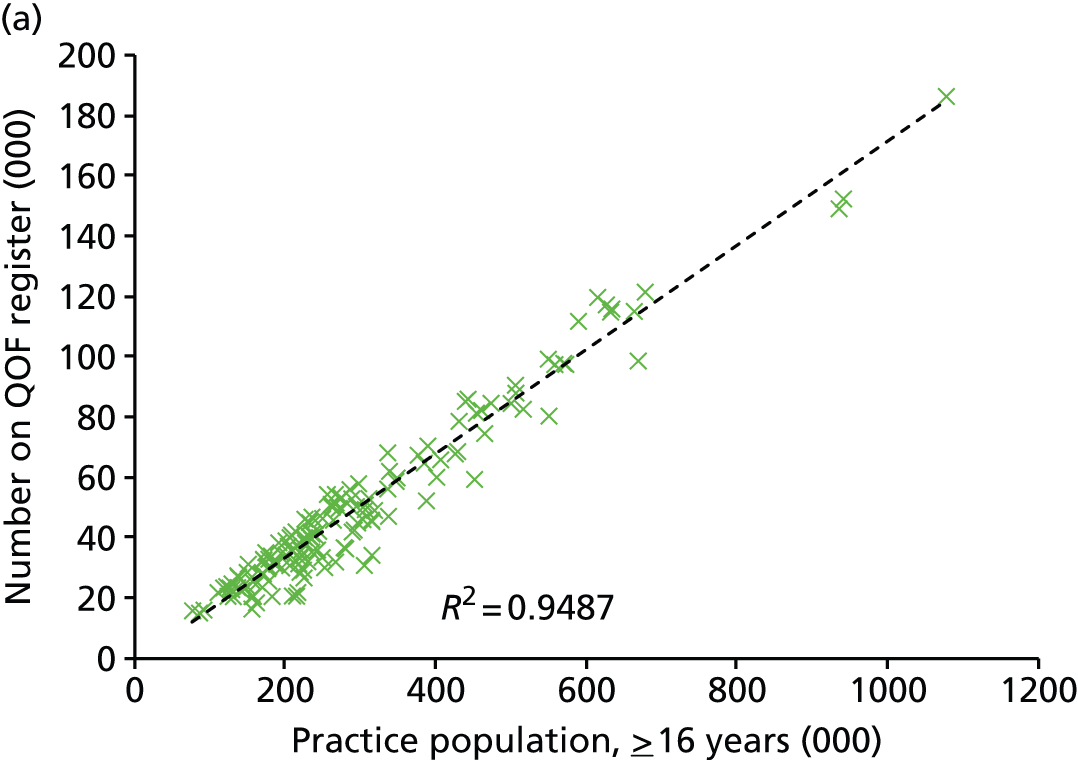
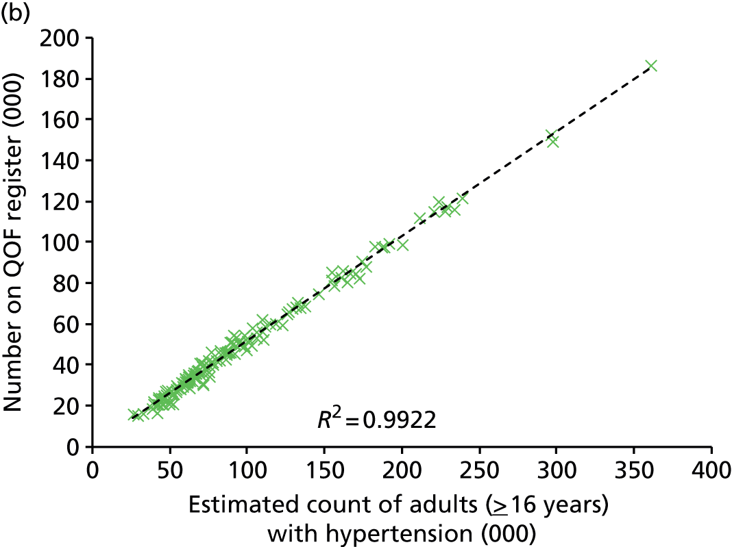
Interestingly, although we have evidence of high levels of unmet need (the QOF ‘all-ages’ rate of 13.6% is broadly equivalent to about 17% for adults aged 16 years and older, which is far short of the estimated 32.5% of people aged ≥ 16 years with hypertension), there is, nevertheless, a very strong relationship between, on the one hand, the modelled estimate of the number of people with hypertension and, on the other hand, the number of patients with hypertension who are ‘known’ to primary care services. This, we would argue, is strongly indicative that the modelled estimates are fundamentally robust and that case finding is relatively consistent at both PCT and practice level. It does not, in other words, seem plausible that any misestimation of the number of people with hypertension should be so effectively balanced by an opposite and equal variation in rates of case finding.
Stroke
The final QOF register which provides relevant comparator data on CVD-related morbidity is the Stroke and Transient Ischaemic Attack (TIA) Disease Register. In this case only one prevalence rate is available as a potential needs indicator, based on the number of people reporting a stroke (including cerebral haemorrhage and cerebral thrombosis) as a LSI. As shown in Table 16, the resulting prevalence rate is significantly lower than the number of patients on the QOF stroke and TIA disease register. This reflects the pattern found with diabetes, CHD and hypertension, and, once again, no doubt reflects how respondents have interpreted whether an illness ‘has troubled you over a period of time, or that is likely to affect you over a period of time’.
| QOF register | Practice population (all ages) | Patients on the register | QOF prevalence rate, % |
|---|---|---|---|
| Stroke and TIA 2010–11 | 55,169,643 | 944,099 | 1.7 |
| Stroke and TIA 2011–12 | 55,525,732 | 964,273 | 1.7 |
| Potential stroke needs indicator (2001 ADS population ≥ 16 years = 44,813,241) | |||
| Modelled prevalence | Predicted cases (≥ 16 years) | Prevalence rate, % (95% CI) | |
| As a LSI | 424,768 | 0.95 (0.78 to 1.14) | |
This disparity does not, of course, mean that local estimates of the number and proportion of people living with stroke as a LSI cannot be used to proxy variations in the need for appropriate health-care services. Indeed, as with respect to the other conditions for which we have ‘LSI’ estimates, the very fact that the condition ‘troubles’ respondents implies a need for health care. More generally, however, the issue is whether or not the relationship between reporting stroke ‘as a LSI’ and the need for relevant health-care services is socially and demographically invariant.
In fact, as shown in Table 17, the number of people estimated to be living with stroke as a LSI condition is very strongly predictive of PCT-level variations in the number of people on the QOF register. Thus, whereas the number of people in ‘at-risk’ populations aged ≥ 16 years predicts only 88.3% of the variation in QOF registrations, the estimated number of people living with stroke as a ‘LSI’ predicts 98.3% of the variation. Figure 3 graphically illustrates the far better relationship achieved by the needs indicator compared with using a simple ‘at-risk’ population. This is also apparent at practice level, where practice-level counts of people aged ≥ 16 years explains 69.4% of the variation in the number of people QOF registered, compared with 91.4% of variation explained by modelled estimates of the number of people in each practice living with stroke as a LSI.
| Denominator population | Prevalence rate, % | Registrations per expected case | Count correlation | |||
|---|---|---|---|---|---|---|
| Mean | Minimum–maximum | Variation | R | % R2 | ||
| Total QOF population (all ages) | 1.74 | – | – | – | 0.933 | 87.0 |
| Total population ≥ 16 years | 2.15 | – | – | – | 0.939 | 88.3 |
| Adults reporting stroke as a LSI | 0.95 | 2.23 | 1.69–2.76 | 1.63 | 0.991 | 98.3 |
FIGURE 3.
Primary care trust-level QOF registrations against population and modelled estimate denominators: stroke. (a) Population (≥ 16 years) against QOF registrations, 2011–12; and (b) estimate (≥ 16 years) against QOF registrations, 2011–12.
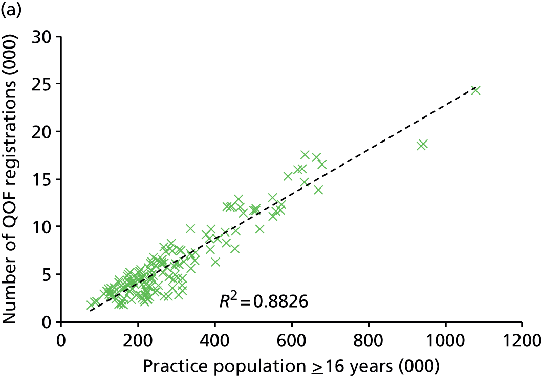
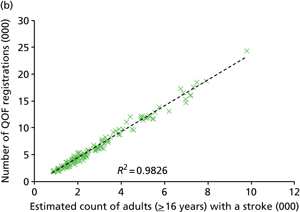
Comparison with existing prevalence estimates
It is necessary to conclude this assessment of the ‘competence’ of our modelled needs indicators by comparing them with the only available alternative measures of modelled prevalence, namely the various prevalence estimates published by PHE. Prevalence models for hypertension and CVD were produced at around the same time that we commenced this project. 213,214 As in our approach, these models were developed from data from the HSfE. However, different modelling strategies have been used (see Chapter 3, Introduction). Moreover, the existing PHE estimates have been made available at PCT level and are in the process of being converted to CCG level. However, they are not available for LSOAs and MSOAs and, therefore, cannot be used to model variation in utilisation at a finer geographical level.
Table 18 compares our modelled estimates with those of PHE for each of the four conditions for which we have appropriate QOF registration data. The ‘need estimate only’ correlation (r) and associated ‘proportion of variance explained’ (% R2) statistics describe how well (a) the PHE and (b) our Plymouth estimates of health service need predict PCT-level variations in QOF registration rates. In each case the Plymouth estimate significantly outperforms the equivalent PHE estimate, often markedly so. For instance, whereas published PHE modelled estimates of the prevalence rate for stroke explain 52.4% of the variation in PCT-level QOF registration rates, the Plymouth estimate explains 87.4% of variation.
| Condition | Need estimate only | Full linear regression model predicting utilisation | |||||||
|---|---|---|---|---|---|---|---|---|---|
| % R2 | Significant coefficients (standardised) | ||||||||
| R | % R2 | Need | Asian | Black | Pop < 50 | IMD | Rural | ||
| Diabetes 2012–13 CCGs (n = 211) | |||||||||
| (a) PHE estimates | 0.763 | 58.0 | 67.3 | 0.386 | 0.307 | – | –0.595 | 0.419 | – |
| (b) Plymouth estimates | 0.804 | 64.5 | 75.1 | 0.720 | 0.463 | –0.112 | –0.239 | – | – |
| CHD 2011/12 PCTs (n = 151) | |||||||||
| (a) PHE estimates | 0.768 | 58.7 | 87.4 | –0.212 | – | –0.310 | –1.071 | 0.634 | –0.105 |
| (b) Plymouth estimates | 0.930 | 86.3 | 89.6 | 0.734 | 0.106 | –0.192 | –0.160 | – | – |
| Hypertension 2011–12 PCTs (n = 151) | |||||||||
| (a) PHE estimates | 0.889 | 78.9 | 86.4 | – | 0.092 | 0.117 | –1.281 | 0.293 | –0.170 |
| (b) Plymouth estimates | 0.931 | 86.6 | 89.3 | 1.359 | – | 0.113 | 0.286 | – | –0.114 |
| Stroke 2011–12 PCTs (n = 151) | |||||||||
| (a) PHE estimates | 0.724 | 52.4 | 90.6 | –0.122 | –0.083 | –0.189 | –0.975 | 0.404 | – |
| (b) Plymouth estimates | 0.935 | 87.4 | 90.4 | 0.273 | –0.075 | –0.154 | –0.588 | 0.213 | – |
As they are, in and of themselves, better predictors of variations in QOF registrations rates, it is highly likely that the Plymouth estimates are better indicators of underlying morbidity across all four conditions. This is reinforced by the evidence given on the right-hand side of Table 18, which describes the outcome of stepwise-selection-based linear regression modelling of QOF registration rates relative to underlying per-capita morbidity (‘need’) and a series of measures which attempt to capture the sociodemographic and geographical characteristics of PCTs. Specifically, the percentage of PCT populations of Asian or British Asian ethnicity (‘Asian’); the percentage of black or black British ethnicity (‘black’); the percentage aged < 50 years (‘pop < 50’); a measure of average deprivation for the PCT; and, finally, the percentage of PCT populations living in LSOAs defined as ‘rural’.
The first column describes the total variation in PCT-level QOF registration rates that is explained by the final linear regression model, while the remaining columns give the standardised coefficient values for all model parameters. For instance, with respect to diabetes (the only one of the conditions for which PHE estimates are available for CCGs), when using currently available PHE prevalence estimates, an initial ‘need estimate only’ % R2 value of 58.9% rises to 67.3% once ‘Asian’, ‘pop < 50’ and ‘IMD’ factors are included in the model. In this case the parameter coefficients suggest that QOF registration was higher than expected in PCTs serving more deprived populations (with higher IMD scores) and with a higher percentage of people of Asian or British Asian ethnicity, and lower than might have been expected in PCTs with younger populations.
This can be compared with the model based on Plymouth estimates, which explains a somewhat larger 75.1% of the variation in PCT-level QOF registration rates and, crucially, incorporates a somewhat different set of parameter estimates in the final predictive model. The effect of deprivation (IMD) disappears, although rates remain higher than expected in PCTs serving populations with a higher percentage of people of Asian ethnicity, and lower than expected in PCTs serving younger populations. There is now also some evidence of relative under-registration in PCTs with a higher percentage of people of black or black British ethnicity.
There is much to glean from this table, but two sets of interrelated observations stand out. First, the Plymouth need estimates are always better predictors of variations in QOF registration rates than the PHE estimates and, moreover, whereas the former are generally incorporated as the most important factor in the linear regression model, the PHE need estimates behave erratically. The PHE need estimate is thus excluded from the hypertension model, and incorporated as a negative parameter in both the CHD and the stroke models. Second, although the final linear regression models tend to explain a similar amount of the variation of PCT-level QOF registration rates, the factors included in the models do differ. Most significantly, deprivation is always incorporated as a positive factor in the PHE models, but appears in only one of the Plymouth models (for stroke). The point here is that if, as seems extremely likely, the PHE estimates fail to fully capture variations in the underlying prevalence of these four conditions, then little can be concluded from any analysis of variations in use relative to need. In this case, for instance, the apparent relatively higher-than-expected rates of QOF registration in areas of high deprivation are almost certainly spurious.
In contrast, using the Plymouth estimates offers a very much more satisfactory explanation of variations in QOF registration rates across all four conditions. In particular, the fact that one gets consistently large and positive standardised ‘need’ parameter values and, conversely, almost invariably much smaller parameter values associated with all other parameters except ‘pop < 50’ is strongly suggestive of measures which genuinely capture variations in underlying morbidity.
There is every reason, therefore, to believe that these needs indicators can be used to study variations in access to, and uptake of, health services relative to need. This is the subject of Variations in the use of cardiovascular care relative to need, though it should be noted that the foregoing discussion also serves to demonstrate the intrinsic value of the estimates to the public health community and commissioners of local NHS services. With precisely the same methodology being used to produce prevalence rates for a wide range of geographical and organisational units (LSOAs, MSOAs, upper- and lower-tier LAs, regions, general practices, PCTs, CCGs and SHAs), many of which are to be made available via PHE’s Local Health website (www.localhealth.org.uk/), these prevalence rates constitute a robust evidence base for future investigations into health service equity at a variety of scales and using a variety of measures of service use, performance and outcomes.
Conclusion
This part of the chapter has been primarily concerned with (a) identifying which of the range of prevalence rates available for diabetes, CHD, hypertension and stroke should be used as needs indicators, and (b) establishing whether or not there is prima facie evidence that the selected indicators are sufficiently robust and unbiased to provide a suitable basis for assessing variations in health service utilisation relative to need. As noted in The lack of a gold standard, in one sense the latter is an impossible goal, as there can be no definitive empirical proof that the modelled estimates accurately describe variations in the underlying morbidity of populations. Nevertheless, the extent to which variations in the number of patients on the various QOF registers are so strongly related to estimates of the underlying number of people with relevant conditions lends some initial support to the veracity of the estimates.
The count-based correlations and associated R2 statistics considered above are, however, of only limited utility to this study. The overwhelming significance of the relative size of different PCTs and practices on the number of people who are QOF registered (or who utilise other health services) means they impart an impression of strength of association which is not matched when rates, rather than counts, are compared. Standard measures of inequality such as the Gini coefficient (or, for that matter, other measures, such as the Theill and Atkinson Indices which similarly aim to describe how an outcome, such as use of health-care services, is distributed between cohorts481–484) are also of only limited analytical utility.
In terms of Gini coefficients, access to primary health care at PCT level (as measured by QOF registration relative to our condition-specific needs estimates) appears very equitable. With a scale that runs from 0 (complete equality) to 1 (complete inequality), the coefficients for diabetes, CHD, hypertension and stroke are 0.0497, 0.0884, 0.0358 and 0.0549, respectively. Indeed, in each case the ‘Lorenz curve’, which plots the cumulative proportion of PCT-level QOF registrations against the cumulative number of people in PCTs estimated to have each condition, is very close to the 45° ‘line of equality’. As might be expected, greater inequalities of access to primary health care is apparent at practice level, with Gini coefficients for diabetes, CHD, hypertension and stroke of 0.1105, 0.1290, 0.0948 and 0.1393, respectively.
Gini coefficients and associated plots of health-care inequality (using Lorenz curves) can thus be used to illustrate how, in general terms, equity of use relative to estimated need varies between different conditions (Figure 4) or, for each condition, between different stages of the care pathway (Figure 5), but this does not help us to understand the sociodemographic dimensions of inequalities. To that end ‘concentration indices’ have often been used which, in the present context, would describe the extent to which inequalities in use-to-need ratios are associated with particular factors,483,485 generating, for instance, measures of ‘deprivation-related’ health-care inequality or ‘age-related’ health-care inequality. Our preferred approach, however, has been to utilise regression models to isolate and quantify the independent effect of the different factors, that is, once the role of other factors in predicting variations in use-to-need ratios has been allowed for.
FIGURE 4.
Condition-specific inequality (Lorenz) curves for QOF registrations relative to need.

FIGURE 5.
Condition-specific inequality (Lorenz) curves for QOF registrations and prescribing and secondary programme budget expenditure. (a) Diabetes; (b) CHD; (c) hypertension; and (d) stroke.
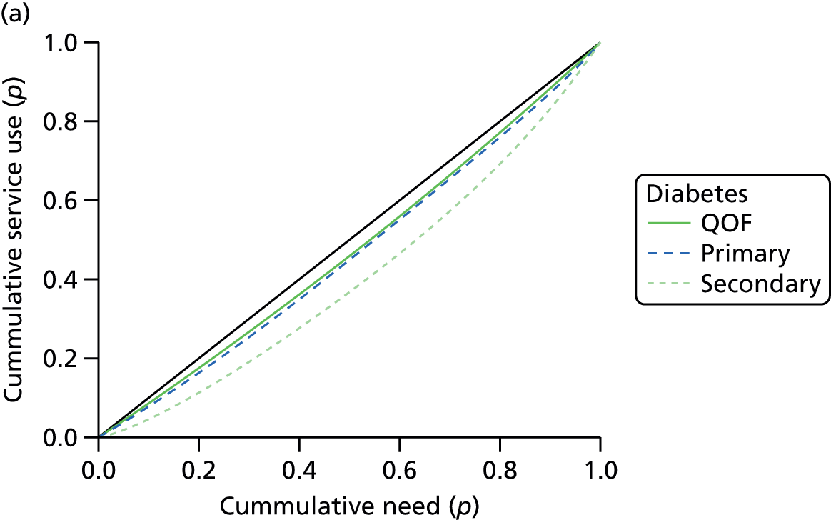
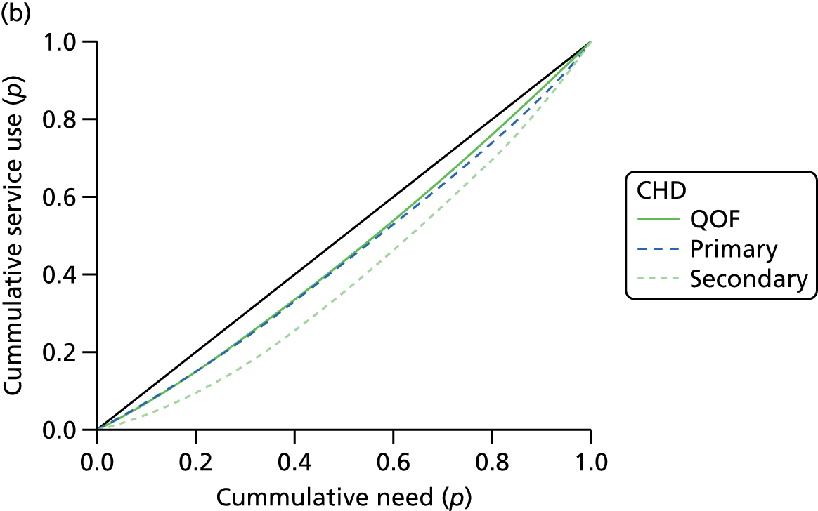
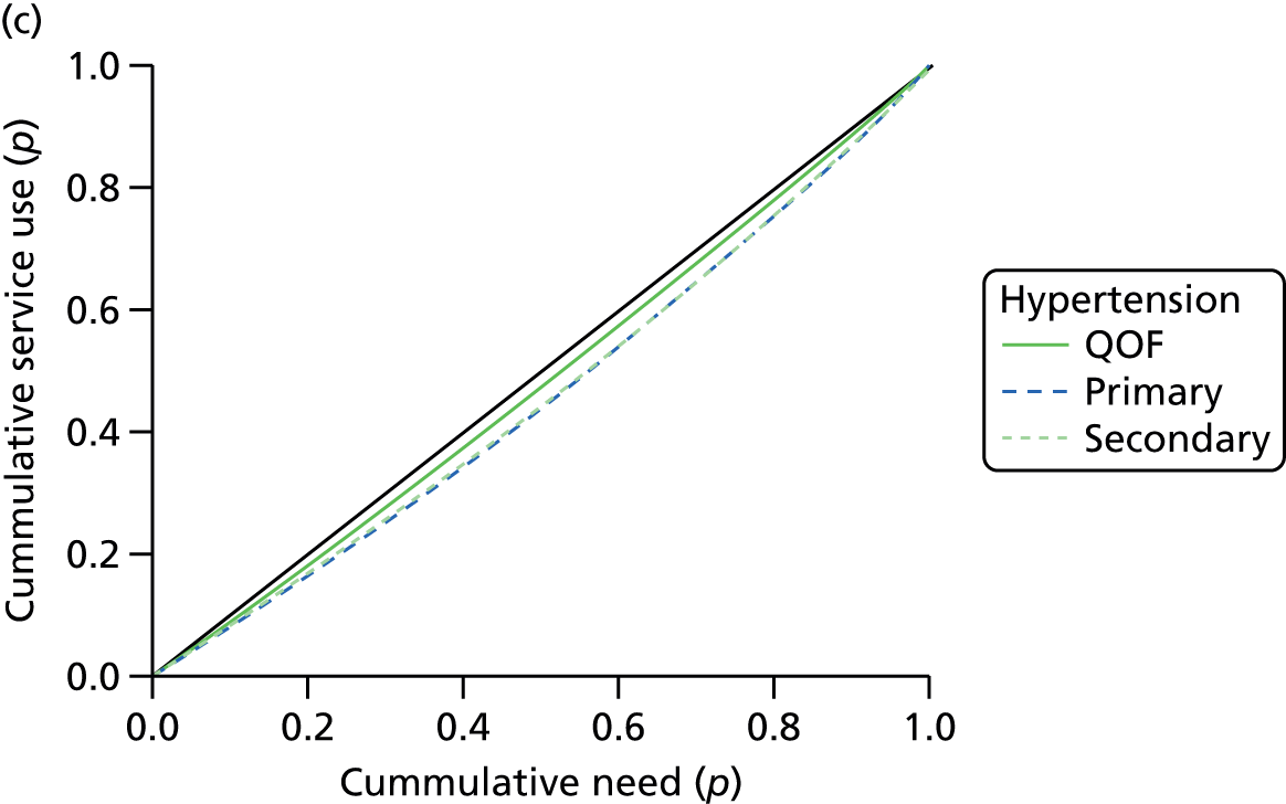

Thus, in the next section, which turns to consider evidence of equity with respect to the uptake of services associated with the care of patients with diabetes, CHD, hypertension and stroke, we examine how per-capita QOF registration rates, along with other per-capita utilisation rates, compare with per-capita estimates of underlying morbidity. Linear regression modelling is used to establish whether measures summarising the age composition, ethnicity, deprivation or rurality (a systematic as opposed to random measure of geography) of practices and PCTs can account for any of the variation in the relationship between estimated service need and recorded service use. An important aspect of this modelling is to construct a coherent and convincing narrative which demonstrates that the modelled estimates capture as much as possible of any systematic sociodemographic and spatial variation in underlying morbidity, ensuring that any remaining unexplained variation in the relationship between use and needs is attributable to patterns of unmet need rather than to inadequacies in the underlying need estimates. This is crucial to the entire project, as any systematic failure of the needs indicator will result in spurious relationships between use and need.
Variations in the use of cardiovascular care relative to need
Introduction
As noted in Chapter 1 (see Implications for research), in order to capture the possibility that inequalities in access and use occur in different ways at different stages of the care pathway, we have explored evidence with respect to presentation, primary management and secondary management (Table 19). For each of the disease conditions under consideration, variations in presentation are explored by examining variations in QOF-recorded prevalence relative to modelled prevalence. Primary management is measured by examining rates of prescribing and Programme Budget Category (PBC) expenditure on prescribing. 486 British National Formulary (BNF)487 codes for drugs examined in each category are listed in Tables 20–23. Finally, variations in secondary management are examined with respect to elective and emergency admissions, the utilisation of specific procedures, and PBC secondary expenditure.
| Condition | Presentation | Primary management | Secondary management |
|---|---|---|---|
| Diabetes | QOF-registered diabetes (2011–12) | Prescribing of diabetic use drugs; insulin; other anti-diabetic drugs PBC prescribing (£) for diabetes |
Hospital admission for diabetes: any diagnosis; main diagnosis; main diagnosis for emergency admission PBC diabetes secondary (£) |
| CHD | QOF-registered CHD (2011–12) | Prescribing of ACE inhibitors; aspirin; beta-blockers; bendroflumethiazide; lipid-lowering drugs; statins PBC prescribing (£) for CHD |
Hospital admission for angina or acute MI: any diagnosis; main diagnosis; main diagnosis for emergency admission Hospital admission for CABG procedure: main admission; emergency admission Hospital admission for PCI: main admission; emergency admission PBC CHD secondary (£) |
| Hypertension | QOF-registered hypertension (2011–12) | Prescribing of ACE inhibitors; ARBs; calcium channel blockers; thiazide diuretics PBC prescribing (£) for problems of circulation; CHD; cerebrovascular; other circulation |
Hospital admission for hypertension: any diagnosis; main diagnosis; main diagnosis for emergency admission PBC secondary (£) for problems of circulation; CHD; cerebrovascular; other circulation |
| Stroke | QOF-registered stroke and TIA (2011–12) | Prescribing of oral anticoagulants; antiplatelets; warfarin PBC prescribing (£) for cerebrovascular |
Hospital admission (stroke as main diagnosis) Emergency admission (stroke as main diagnosis) PBC cerebrovascular secondary (£) |
Variations in use relative to need: diabetes
Diabetes has been included in the study for reasons outlined in Chapter 1 (see Aims and objectives), not least because it is an important risk factor for CHD, hypertension and stroke. Table 20 shows the results of full linear regression modelling to predict per-capita service use for diabetes at PCT level, and Table 21 predictions at general practice level (n = 6984). The ‘need’ parameter is the estimated per-capita rate of diabetes, using the LSI definition. The first thing to note is that, taken on its own, the underlying prevalence of diabetes explains 62.1% of the variation of PCT-level QOF registration rates, suggesting that a good deal of the variation in presentation can be explained by underlying need. As might be expected, the percentage of variation that is predicted at practice level is smaller (44.5%).
| Per-capita service use | Need estimate only | Full linear regression model predicting utilisation | |||||||
|---|---|---|---|---|---|---|---|---|---|
| % R2 | Significant coefficients (standardised) | ||||||||
| R | % R2 | Need | Asian | Black | Pop < 50 | IMD | Rural | ||
| QOF register 2011–12 | 0.789 | 62.1 | 75.6 | 0.623 | 0.559 | – | –0.394 | – | – |
| Prescribing | |||||||||
| Diabetic use (NIC) | 0.674 | 45.0 | 60.1 | 0.239 | 0.643 | – | –0.758 | 0.302 | – |
| Insulin (NIC) | 0.574 | 32.5 | 49.7 | 0.531 | 0.335 | –0.451 | – | – | 0.174 |
| Other antidiabetic (NIC) | 0.546 | 29.3 | 45.4 | 0.506 | 0.406 | – | – | – | – |
| PBC prescribing expenditure486 | |||||||||
| Diabetes | 0.612 | 37.0 | 51.4 | 0.562 | 0.461 | –0.154 | – | – | – |
| Diabetes (ICD-10: E10–14) patients488 | |||||||||
| Any diagnosis; all patients | 0.718 | 51.2 | 63.8 | 0.690 | 0.139 | –0.452 | – | 0.310 | –0.0194 |
| Main diagnosis; all patients | 0.331 | 10.4 | 18.0 | 0.195 | –0.285 | – | – | – | – |
| Main diagnosis; emergency | 0.504 | 25.4 | 45.6 | 0.277 | –0.284 | – | – | 0.477 | –0.168 |
| PBC secondary expenditure486 | |||||||||
| Diabetes | 0.123 | – | 27.8 | – | –0.241 | 0.451 | – | 0.345 | – |
| Per-capita service use | Need estimate only | Full linear regression model predicting utilisation | |||||||
|---|---|---|---|---|---|---|---|---|---|
| % R2 | Significant coefficients (standardised) | ||||||||
| R | % R2 | Need | Asian | Black | Pop < 50 | IMD | Rural | ||
| QOF register 2011–12 | 0.667 | 44.5 | 57.6 | 0.604 | 0.391 | –0.128 | – | 0.089 | 0.062 |
| Prescribing | |||||||||
| Diabetic use (NIC) | 0.509 | 25.9 | 37.7 | 0.366 | 0.344 | –0.194 | –0.077 | 0.243 | 0.084 |
| Insulin (NIC) | 0.424 | 17.9 | 25.8 | 0.437 | 0.127 | –0.282 | 0.127 | 0.165 | 0.138 |
| Other antidiabetic (NIC) | 0.416 | 17.3 | 33.6 | 0.183 | 0.427 | –0.002 | –0.191 | 0.273 | – |
| Diabetes (ICD10: E10–14) patients488 | |||||||||
| Any diagnosis; all patients | 0.668 | 44.6 | 52.6 | 0.590 | 0.156 | –0.262 | – | 0.228 | – |
| Main diagnosis; all patients | 0.290 | 8.4 | 16.2 | 0.319 | –0.186 | –0.043 | 0.206 | 0.215 | 0.040 |
| Main diagnosis; emergency | 0.255 | 6.5 | 18.9 | 0.264 | –0.142 | –0.063 | 0.227 | 0.275 | – |
Although underlying prevalence accounts for the greater proportion of presentation relative to need at both PCT and practice levels, additional factors increase the variance explained (to 75.6% between PCTs and 57.6% between practices). As indicated by the standardised coefficients given in Table 20, both the proportion of people of Asian or British Asian ethnicity and the percentage of people under the age of 50 years contribute to the explanation of variations in PCT-level QOF registration rates. At practice level (see Table 21), diabetes registration is also significantly higher than one might expect among Asian populations. However, registrations are also higher in deprived and rural communities, and lower in practices with larger percentages of black populations.
As one moves up the care pathway, the percentage of variance that can be explained by either estimated prevalence or additional factors falls. With respect to diabetic prescribing items, for example, < 50% of the variation at PCT level can be explained by underlying need alone. However, once additional variables are factored in, prediction improves [e.g. to 60.1% for PCT-level variations in prescribing of diabetic drugs (BNF 6.1487)]. Prediction is far poorer at practice level (25.9% for diabetic drugs). Again, significantly higher rates of prescribing among Asian populations appear to play an important role in improving explanation of overall variance. Here, however, additional factors emerge as explanatory variables. Prescribing rates are significantly higher in deprived and rural communities, and lower in practices with larger percentages of black populations. However, younger communities continue to appear to be underserved, albeit with mixed results, with practices with a higher percentage of adults under the age of 50 years being less likely to prescribe diabetic drugs (BNF 6.1487) and other antidiabetic drugs (BNF 6.1.2487) but more likely to prescribe insulin (BNF 6.1.1487). It is important to note that, although these coefficients are significant (i.e. p < 0.05), their contribution, compared with underlying need, is small.
With regard to secondary care, the direction of some of these coefficients changes. Importantly, PCTs and practices with a higher percentage of Asian populations now have lower-than-expected rates of admission (elective and emergency) for a main diagnosis of diabetes and lower PBC expenditure on the disease. By contrast, PCTs with a higher percentage of black populations have higher PBC expenditure on hospital care (data available at PCT level only). This suggests that relative mix of care may be a key factor in understanding variations in the appropriateness of NHS care provided. High rates of presentation and prescribing among Asian populations and lower-than-expected rates of secondary care suggest that, among this population, diabetes may be better managed within primary and community settings than among other population groups. Against this, more deprived PCTs and practices have higher-than-expected rates of both prescribing and secondary care (particularly with respect to emergency admission for diabetes as a main diagnosis); and PCTs and practices with higher black populations have lower utilisation rates than expected in both primary and secondary care.
Finally, it is worth pointing out that, although full linear regression modelling can throw light on variations in access and use according to population characteristics, a significant percentage of variation remains unexplained. This may be indicative of random variation (i.e. a ‘postcode lottery’). However, as we explore with respect to CHD, systematic regional differences in use relative to need may complicate the picture. This is discussed in the following section.
Variations in use relative to need: coronary heart disease
Variations in the presentation of coronary heart disease
At the PCT level, estimated prevalence of CHD (based on the clinical evidence definition) explains a very high percentage (86.3%) of variations in QOF registrations (Table 22). Once additional factors are accounted for, 89.6% of variance can be explained. At practice level (n = 7848), variance explained by underlying need (65.4%) increases to 70.5% in the full linear regression model (Table 23). Again, registration (relative to need) is significantly higher than one might expect among Asian populations and significantly lower in PCTs with higher percentages of black and younger populations at both scales of analysis. These results correspond with those of several published studies that note significantly higher levels of presentation among South Asians227,233 and lower CHD QOF registrations than expected among younger people. 222,233 The lack of evidence on socioeconomic differences in registration also accord with the rather mixed findings reported in Chapter 2 (see Variations in access to and use of cardiovascular care in England: what does the evidence tell us? and The direction of inequality, Presentation of cardiovascular problems), some studies finding that the gap between modelled and registered prevalence was higher among practices in more deprived areas224 and others finding that people from less advantaged communities are more likely to present to, for example CHD risk-screening programmes. 225,228 We have not found published evidence that suggests that black populations are less likely to present for CHD.
| Per-capita service use | Need estimate only | Full linear regression model predicting utilisation | |||||||
|---|---|---|---|---|---|---|---|---|---|
| % R2 | Significant coefficients (standardised) | ||||||||
| R | % R2 | Need | Asian | Black | Pop < 50 | IMD | Rural | ||
| QOF register 2011–12 | 0.930 | 86.3 | 89.6 | 0.734 | 0.106 | –0.192 | –0.160 | – | – |
| Prescribing | |||||||||
| ACE inhibitors (NIC) | 0.836 | 69.7 | 75.6 | 0.575 | 0.146 | – | –0.444 | – | – |
| Aspirin (NIC) | 0.912 | 83.0 | 86.5 | 0.745 | 0.194 | –0.117 | –0.250 | – | – |
| Beta-blockers (NIC) | 0.869 | 75.3 | 79.7 | 0.790 | – | –0.142 | –0.136 | – | |
| Bendroflumethiazide (NIC) | 0.773 | 59.5 | 66.6 | 0.538 | – | – | –0.248 | – | 0.142 |
| Lipid-lowering drugs (NIC) | 0.654 | 42.4 | 45.0 | 0.527 | – | – | –0.281 | – | –0.273 |
| Statins (NIC) | 0.659 | 43.1 | 43.1 | 0.659 | – | – | – | – | – |
| PBC prescribing expenditure486 | |||||||||
| CHD | 0.628 | 39.0 | 42.7 | 0.696 | – | – | – | – | –0.212 |
| Angina or acute MI (ICD-10: I20–21) patients (main diagnosis)488 | |||||||||
| Any admissions | 0.805 | 64.6 | 64.6 | 0.805 | – | – | – | – | – |
| Emergency admissions | 0.821 | 67.3 | 67.3 | 0.821 | – | – | – | – | – |
| CABG (OPCS-4 operation codes K40–46) patients490 | |||||||||
| Any admissions | 0.593 | 34.8 | 40.4 | 0.430 | 0.279 | – | –0.412 | – | – |
| Emergency admissions | 0.200 | 4.0 | 5.9 | – | – | –0.188 | – | 0.68 | – |
| PCI (OPCS-4 operation codes K49–50, K75) patients490 | |||||||||
| Any admissions | 0.543 | 35.2 | 42.4 | 0.242 | 0.361 | – | –0.649 | – | – |
| Emergency admissions | 0.326 | 10.0 | 12.4 | 0.437 | 0.206 | – | – | – | – |
| PBC secondary expenditure486 | |||||||||
| CHD | –0.013 | – | – | – | – | – | – | – | – |
| Per-capita service use | Need estimate only | Full linear regression model predicting utilisation | |||||||
|---|---|---|---|---|---|---|---|---|---|
| % R2 | Significant coefficients (standardised) | ||||||||
| R | % R2 | Need | Asian | Black | Pop < 50 | IMD | Rural | ||
| QOF register 2011–12 | 0.809 | 65.4 | 70.5 | 0.680 | 0.102 | –0.219 | –0.117 | – | – |
| Prescribing | |||||||||
| ACE inhibitors (NIC) | 0.538 | 28.9 | 30.8 | 0.403 | 0.059 | – | –0.217 | – | – |
| Aspirin (NIC) | 0.752 | 56.6 | 61.2 | 0.647 | 0.195 | –0.115 | –0.177 | – | 0.058 |
| Beta-blockers (NIC) | 0.672 | 45.1 | 51.0 | 0.433 | – | –0.161 | –0.258 | – | –0.070 |
| Bendroflumethiazide (NIC) | 0.534 | 28.5 | 32.8 | 0.497 | – | 0.063 | –0.101 | –0.132 | 0.059 |
| Lipid-lowering drugs (NIC) | 0.535 | 28.6 | 32.2 | 0.140 | 0.059 | –0.084 | –0.525 | 0.200 | –0.166 |
| Statins (NIC) | 0.534 | 28.5 | 31.9 | 0.117 | 0.065 | –0.076 | –0.550 | 0.225 | –0.137 |
| Angina or acute MI (ICD-10: I20–21) patients (main diagnosis)488 | |||||||||
| Any admissions | 0.620 | 38.4 | 42.1 | 0.596 | 0.171 | –0.163 | – | 0.084 | 0.083 |
| Emergency admissions | 0.614 | 37.7 | 41.6 | 0.597 | 0.182 | –0.168 | – | 0.080 | 0.066 |
| CABG (OPCS-4 operation codes K40–46) patients490 | |||||||||
| Any admissions | 0.291 | 8.5 | 12.6 | 0.376 | 0.156 | – | – | –0.197 | 0.067 |
| Emergency admissions | 0.077 | 0.6 | 0.8 | 0.118 | 0.030 | 0.031 | – | –0.055 | –0.037 |
| PCI (OPCS-4 operation codes K49–50, K75) patients490 | |||||||||
| Any admissions | 0.206 | 4.2 | 15.7 | 0.326 | 0.228 | 0.154 | –0.069 | –0.280 | 0.166 |
| Emergency admissions | 0.245 | 6.0 | 8.6 | 0.153 | 0.155 | – | –0.205 | – | 0.031 |
Variations in the primary management of coronary heart disease
The modelled needs estimates explain far less of the variance in primary management at practice level than at PCT level (e.g. 69.7% and 28.9%, respectively, of variation in prescribing of ACE inhibitors). Again, prescribing data at both scales of analysis suggest higher-than-expected rates among Asian populations and lower-than-expected rates (with the exception of beta-blockers and bendroflumethiazide) among younger and black populations, though it is important to note that these additional factors explain a relatively small proportion of overall variance. Variations in prescribing according to deprivation and rurality are mixed. Practices serving more deprived populations prescribe less bendroflumethiazide than expected but more lipid-lowering drugs, including statins, while practices serving rural populations prescribe higher-than-expected levels of bendroflumethiazide and aspirin, but lower levels of beta-blockers, lipid-lowering drugs and statins.
Again, these findings accord with those of some but not all published studies (see Chapter 2, Variations in access to and use of cardiovascular care in England: what does the evidence tell us? and The direction of inequality, Primary management of cardiovascular disease). Equal or better primary management of CHD for South Asian populations has been reported in several studies,144,198,229,253,258,279,281 as have lower rates of prescribing among black populations. 241,258 The findings of published studies on variations in primary management by socioeconomic status are, like our own results, mixed, with some finding lower prescribing rates among deprived populations233,252,253,262,263 and others finding no difference or a positive association in prescribing and referral rates by social deprivation. 144,241,256,258,264,266,267 Our finding that practices serving younger populations have significantly lower prescribing rates for CHD drugs than expected does conflict with the results of published studies, which report consistent evidence that rates of CHD prescribing are lower than expected among older people. 191,192,195,252,253,258,272,273,275
Variations in the secondary management of coronary heart disease
With respect to secondary management of CHD, the percentage of variance explained by both underlying need and the full model falls away significantly. This is likely to reflect the fact that ‘within-system’ management is a more important determinant of need for specialist CHD services than underlying prevalence. However, in contrast to our findings on diabetes, significantly higher rates of presentation and prescribing in South Asian populations are not accompanied by lower rates of inpatient use. Practices with high South Asian populations have higher-than-expected rates of admissions for CABG and PCI, the latter on an elective and emergency basis. This corresponds with the results of several studies that find higher cardiac procedure rates among South Asian populations,144,217,295,307,310 although some studies suggest lower rates of use relative to need,306 particularly for cardiac rehabilitation297,309 (which we do not have data for).
In other respects, we have very little evidence of systematic bias in the secondary management of CHD. Practices serving deprived populations have higher-than-expected rates of emergency admissions for CABG, a trend that has been previously observed,245,259,265 although it is important to note that such studies find that there is little evidence to suggest that the clinical quality of primary care plays a role in this. Again, practices serving younger populations have lower-than-expected rates of elective CABGs and PCIs, a finding that is difficult to square with the results of published studies that suggest that older patients are more likely to be discriminated against with respect to revascularisation. 243,335,337,342,346 This could reflect differences in clinical need, with community and/or primary management being more appropriate and effective among younger patients (it is important to note that the modelled estimate is of underlying prevalence of CHD in the community).
As Hospital Episode Statistics (HES) provide the age and sex of patients (unlike QOF registration and prescribing data), it is possible to explore some of these contradictions (Table 24), although the results are difficult to interpret. First, with the exception of PCI among males, underlying need appears to account for greater variance in younger age cohorts than older cohorts. As a higher correlation (% R2) between need and utilisation implies that utilisation is more ‘equitable’ (insofar as a greater proportion of the variation in rates of use is ‘explained’ by variations in underlying need), this may indicate a greater disconnect between disease prevalence and secondary use of cardiac care at older ages.
| Cohort | Need estimate only | Full linear regression model predicting utilisation | ||||||
|---|---|---|---|---|---|---|---|---|
| % R2 | Significant coefficients (standardised) | |||||||
| R | % R2 | Need | Asian | Black | IMD | Rural | ||
| Acute MI/angina patients | ||||||||
| Males, 50–64 years | 0.507 | 25.2 | 41.1 | 0.574 | 0.511 | –0.338 | NS | NS |
| Males, 65–74 years | 0.416 | 17.3 | 25.7 | NS | NS | NS | 0.512 | NS |
| Males, ≥ 75 years | 0.417 | 16.8 | 19.5 | 0.518 | 0.206 | NS | NS | NS |
| Females, 50–64 years | 0.532 | 28.3 | 40.7 | 0.394 | NS | –0.355 | 0.335 | NS |
| Females, 65–74 years | 0.549 | 30.1 | 42.6 | 0.504 | NS | –0.370 | 0.260 | NS |
| Females, ≥ 75 years | 0.243 | 5.3 | 20.1 | 0.524 | 0.240 | –0.304 | NS | NS |
| CABG patients | ||||||||
| Males, 50–64 years | 0.178 | 3.2 | 21.7 | NS | 0.377 | –0.280 | 0.319 | NS |
| Males, 65–74 years | 0.108 | 1.2 | 7.1 | 0.199 | 0.283 | NS | NS | NS |
| Males, ≥ 75 years | 0.186 | 0.0 | NS | NS | NS | NS | NS | NS |
| Females, 50–64 years | 0.598 | 35.8 | 36.7 | 0.474 | 0.182 | NS | NS | NS |
| Females, 65–74 years | 0.444 | 19.2 | 19.2 | 0.444 | NS | NS | NS | NS |
| Females, ≥ 75 years | 0.117 | 1.4 | NS | NS | NS | NS | NS | NS |
| PCI patients | ||||||||
| Males, 50–64 years | 0.210 | 4.4 | 24.0 | NS | 0.377 | –0.280 | 0.324 | NS |
| Males, 65–74 years | –0.292 | 8.5 | 16.4 | –0.192 | 0.316 | NS | NS | NS |
| Males, ≥ 75 years | –0.430 | 18.0 | 18.0 | –0.430 | NS | NS | NS | NS |
| Females, 50–64 years | 0.562 | 31.6 | 40.5 | NS | NS | –0.202 | 0.685 | NS |
| Females, 65–74 years | 0.401 | 15.5 | 15.5 | 0.401 | NS | NS | NS | NS |
| Females, ≥ 75 years | 0.138 | 1.9 | 8.2 | NS | 0.296 | NS | NS | NS |
For younger women, rates of admission for angina (aged 50–64 and 65–74 years) are higher than expected in deprived areas, as are rates of PCI among women aged 50–64 years. Admissions for angina/acute MI, CABG and PCI are lower than expected for younger black men (aged 50–64 years). Black women of all ages have lower-than-expected rates of angina/MI admissions, and younger black women (aged 50–64 years) have lower-than-expected admissions for PCI. Finally, Asian men under the age of 74 years have higher-than-expected rates of CABG and PCI, while the pattern for Asian women is more mixed.
Is there a ‘geography’ to variations in cardiac care?
As noted above, although the modelled estimates predict a good proportion of variance, particularly at earlier stages of the care pathway, a significant percentage of variation remains unexplained. Although this may be indicative of random variations in medical practice, we propose that there may also be regional variations in utilisation relative to need, which cannot be explained by their compositional (i.e. socioeconomic, sociodemographic and ethnic) characteristics.
Maps of QOF registrations (Figure 6), PBC prescribing (Figure 7), PBC secondary expenditure (Figure 8) and total CHD expenditure (Figure 9) by expected CHD case suggest that the North East has relatively high levels of use of cardiac care, as do parts of the South East and South Central regions. By contrast, the East of England, South West and East and West Midlands have relatively low levels of use. Interestingly, although rurality did not emerge as a significant factor explaining variation in use relative to need, several ‘shires’ (Shropshire, Herefordshire, Worcestershire, Warwickshire, Leicestershire, Northamptonshire, Staffordshire, Derbyshire, Norfolk and Devon) have lower levels of CHD expenditure than expected by their caseloads. This does not appear to be explained by higher levels of prescribing, which might be expected to reduce levels of secondary use in these areas (see Figure 4).
FIGURE 6.
Map of QOF CHD registrations72 per expected CHD case. Contains Ordnance Survey data © Crown copyright and database right 2012.
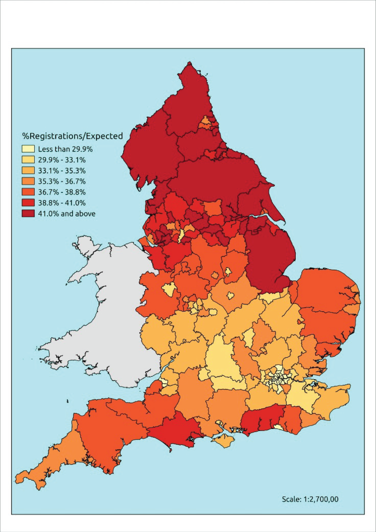
FIGURE 7.
Map of PBC CHD prescribing expenditure486 per expected CHD case. Contains Ordnance Survey data © Crown copyright and database right 2012.
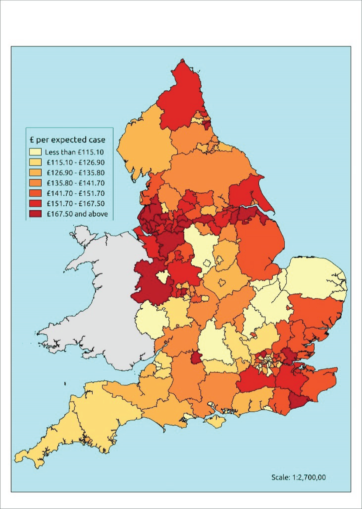
FIGURE 8.
Map of PBC CHD secondary expenditure486 per expected CHD case. Contains Ordnance Survey data © Crown copyright and database right 2012.

FIGURE 9.
Map of PBC CHD total expenditure486 per expected CHD case. Contains Ordnance Survey data © Crown copyright and database right 2012.

One factor that may be worth further investigation is the role of per-capita funding. Referring back to Table 1, which compared allocations for PCTs with the youngest and the oldest demographies, it is worth noting that, apart from North Staffordshire and Devon (which, respectively, received per capita allocations of £1614 and £1506 in 2010–11), all of the shires listed above received < £1500 per head for their Hospital and Community Health Services. By comparison, all of the PCTs (n = 12) in the North East SHA, 12 of 14 in Yorkshire and the Humber, 23 of 24 in the North West, 6 of 8 in the South East, and 30 of 31 in London received higher funding allocations.
Variations in use relative to need: hypertension
Variations in the presentation of hypertension
At the PCT level, estimated prevalence of hypertension (based on the clinical evidence definition) explains a very high percentage (86.6%) of variations in QOF registrations (Table 25). Once additional factors are accounted for, prediction increases to 89.3% of explained variance. At practice level (n = 7848), variance in presentation explained by underlying need (56.1%) increases to 57.6% in the full linear regression model (Table 26).
| Per-capita service use | Need estimate only | Full linear regression model predicting utilisation | |||||||
|---|---|---|---|---|---|---|---|---|---|
| % R2 | Significant coefficients (standardised) | ||||||||
| R | % R2 | Need | Asian | Black | Pop < 50 | IMD | Rural | ||
| QOF register 2011–12 | 0.931 | 86.6 | 89.3 | 1.359 | – | 0.113 | 0.286 | – | –0.114 |
| Prescribing | |||||||||
| ACE inhibitors NIC | 0.852 | 72.5 | 76.2 | 0.971 | – | – | – | 0.133 | –0.134 |
| ARBs NIC | 0.630 | 39.3 | 39.3 | 0.630 | – | – | – | – | – |
| Calcium channel NIC | 0.842 | 70.7 | 75.6 | 0.912 | – | – | – | 0.235 | – |
| Thiazide diuretics NIC | 0.747 | 55.5 | 58.1 | 0.937 | – | 0.256 | – | – | – |
| PBC prescribing expenditure486 | |||||||||
| Problems of circulation | 0.766 | 58.4 | 68.3 | 0.947 | – | – | – | 0.228 | –0.191 |
| CHD | 0.566 | 31.6 | 46.5 | 0.634 | – | –0.207 | – | 0.282 | –0.232 |
| Cerebrovascular | 0.673 | 44.7 | 61.6 | 0.550 | – | –0.332 | – | 0.416 | – |
| Other circulation | 0.876 | 76.5 | 81.1 | 0.987 | – | – | – | 0.117 | –0.99 |
| Hypertensive disease (ICD-10: I10–13, I15) patients488 | |||||||||
| Any diagnosis/all admissions | 0.706 | 49.5 | 57.8 | 0.920 | – | – | – | – | –0.363 |
| Main diagnosis/all admissions | 0.096 | – | 22.3 | 0.546 | – | 0.313 | – | 0.311 | –0.211 |
| Main diagnosis/emergency | –0.132 | – | 22.0 | – | – | – | – | 0.475 | – |
| PBC secondary expenditure486 | |||||||||
| Problems of circulation | 0.461 | 20.7 | 25.9 | 0.701 | 0.188 | – | – | – | –0.214 |
| CHD | 0.152 | – | – | – | – | – | – | – | – |
| Cerebrovascular | 0.343 | 11.2 | 11.2 | 0.343 | – | – | – | – | – |
| Other circulation | 0.215 | – | 12.4 | – | – | – | –0.343 | 0.383 | – |
| Per-capita service use | Need estimate only | Full linear regression model predicting utilisation | |||||||
|---|---|---|---|---|---|---|---|---|---|
| % R2 | Significant coefficients (standardised) | ||||||||
| R | % R2 | Need | Asian | Black | Pop < 50 | IMD | Rural | ||
| QOF register 2011–12 | 0.749 | 56.1 | 57.6 | 0.817 | – | 0.048 | – | 0.081 | –0.052 |
| Prescribing | |||||||||
| ACE inhibitors NIC | 0.531 | 28.2 | 30.4 | 0.404 | – | –0.059 | –0.172 | 0.192 | –0.034 |
| ARBs NIC | 0.472 | 22.5 | 24.5 | 0.090 | 0.146 | – | –0.493 | – | –0.054 |
| Calcium channel NIC | 0.615 | 37.8 | 39.8 | 0.541 | –0.049 | – | –0.106 | 0.177 | – |
| Thiazide diuretics NIC | 0.475 | 22.6 | 23.5 | 0.525 | –0.042 | 0.107 | – | – | –0.035 |
| Hypertensive disease (ICD10: I10–13, I15) patients488 | |||||||||
| Any diagnosis/all admissions | 0.713 | 50.9 | 57.1 | 0.921 | – | –0.039 | 0.134 | 0.162 | –0.130 |
| Main diagnosis/all admissions | 0.089 | 0.8 | 11.9 | 0.163 | 0.092 | 0.136 | –0.140 | 0.250 | –0.069 |
| Main diagnosis/emergency | 0.012 | – | 7.5 | 0.186 | 0.070 | 0.143 | 0.140 | – | –0.078 |
Of the factors that yield significant standardised coefficients at the PCT and practice levels, underlying need accounts for most explainable variation in presentation. Smaller but significant coefficients are found for percentage of black population and percentage of population aged < 50 years, both of which are associated with higher presentation rates than expected. Presentation of hypertension in more rural PCTs and practices is significantly lower than expected, although again the coefficients are small.
Variations in the primary management of hypertension
Different patterns of primary management are observed among Asian populations for hypertension from those for diabetes and CHD. At the practice level of analysis, prescribing rates of calcium channel blockers and thiazide diuretics are lower than expected, although Asian populations receive higher than expected rates of ARBs and the standardised coefficient for ACE inhibitors does not reach significance. The findings for black populations are mixed, with lower-than-expected rates of prescribing of ACE inhibitors being found, against higher-than-expected rates of thiazide diuretics. Results in the published literature on the primary management of hypertension are also mixed (although most studies focus on blood pressure monitoring rather than prescribing). For example, Schofield et al. 283 found that, although blood pressure monitoring was similar across ethnic groups and as good, if not better, for black patients as for white, blood pressure control was poor in Caribbean patients with CHD. Similarly, Lee et al. 280 noted statistically significant short-term reduction in systolic BP in white and black but not in south Asian patients with hypertension. By contrast, Nazroo et al. 198 observed no ethnic inequalities for the clinical outcomes of care for hypertension, while Ashworth et al. 243 report that practices performing less well in terms of blood pressure monitoring were those with higher proportions of black or black British residents in the local population.
With respect to deprivation, both the PCT- and practice-level analyses find higher rates of ACE inhibitor and thiazide diuretics than expected in deprived populations. PBC expenditure is also higher in more deprived PCTs. Although this conflicts with earlier studies,243 others have noted a reduction in the socioeconomic gap in the quality of primary care for CVD over time. 247,248,250 Thus, the results do not challenge expectations. More surprising, perhaps, is our finding that, in more rural practices, levels of prescribing of hypertensive drugs (ACE inhibitors, ARBs and thiazide diuretics) are lower than expected.
Variations in the secondary management of hypertension
Hypertension does not tend to be ‘managed’ within the secondary care setting. Thus, it is not surprising that admissions with the main diagnosis of hypertension are poorly explained by the needs estimates. Interestingly, however, > 50% of variations in admissions where hypertensive disease is recorded in any analysis can be explained by % R2. Although the coefficients are small, it is also worth noting that emergency admissions (main diagnosis hypertensive disease) are significantly higher in practices with higher Asian, black and young populations and lower in more rural practices.
Variations in use relative to need: stroke
At the PCT level, estimated prevalence of hypertension (based on the clinical evidence definition) explains a very high percentage (87.4%) of variations in QOF registrations (Table 27). Once additional factors are accounted for, prediction increases to 90.4% of explained variance. At practice level (n = 7839), variance in presentation explained by underlying need (57.1%) increases to 60.1% in the full linear regression model (Table 28).
| Per-capita service use | Need estimate only | Full linear regression model predicting utilisation | |||||||
|---|---|---|---|---|---|---|---|---|---|
| % R2 | Significant coefficients (standardised) | ||||||||
| R | % R2 | Need | Asian | Black | Pop < 50 | IMD | Rural | ||
| QOF register 2011–12 | 0.935 | 87.4 | 90.4 | 0.273 | –0.075 | –0.154 | –0.588 | 0.213 | – |
| Prescribing | |||||||||
| Oral anticoagulants NIC | 0.677 | 45.5 | 55.3 | – | –0.149 | – | –0.638 | – | – |
| Antiplatelets NIC | 0.843 | 70.9 | 76.4 | 0.927 | – | – | – | 0.171 | –0.118 |
| Warfarin NIC | 0.740 | 54.5 | 63.3 | – | –0.141 | –0.186 | –0.544 | – | – |
| PBC prescribing expenditure486 | |||||||||
| Cerebrovascular | 0.493 | 24.1 | 46.0 | – | – | –0.598 | – | –0.181 | – |
| Stroke (ICD-10: I60–64) patients488 | |||||||||
| Main diagnosis all patients | 0.916 | 83.8 | 86.2 | 0.338 | – | –0.680 | – | 0.244 | – |
| Main diagnosis emergency | 0.917 | 84.0 | 86.6 | 0.323 | –0.083 | –0.646 | – | 0.277 | – |
| PBC secondary expenditure486 | |||||||||
| Cerebrovascular | 0.810 | 65.4 | 69.8 | 0.497 | – | –0.493 | – | 0.292 | –0.192 |
| Per-capita service use | Need estimate only | Full linear regression model predicting utilisation | |||||||
|---|---|---|---|---|---|---|---|---|---|
| % R2 | Significant coefficients (standardised) | ||||||||
| R | % R2 | Need | Asian | Black | Pop < 50 | IMD | Rural | ||
| QOF register 2011–12 | 0.756 | 57.1 | 60.1 | 0.401 | –0.087 | –0.091 | –0.314 | 0.130 | 0.036 |
| Prescribing | |||||||||
| Oral anticoagulants NIC | 0.410 | 16.8 | 22.0 | – | –0.069 | –0.056 | –0.367 | 0.050 | 0.085 |
| Antiplatelets NIC | 0.622 | 38.6 | 43.4 | 0.399 | – | –0.078 | –0.298 | 0.285 | –0.083 |
| Warfarin NIC | 0.626 | 39.2 | 46.2 | 0.192 | –0.113 | –0.082 | –0.366 | 0.032 | 0.059 |
| Stroke (ICD-10: I60–64) patients488 | |||||||||
| Main diagnosis: all patients | 0.647 | 41.9 | 43.2 | 0.377 | –0.025 | – | –0.325 | 0.148 | – |
| Main diagnosis: emergency | 0.647 | 41.8 | 43.2 | 0.385 | –0.030 | – | –0.313 | 0.151 | – |
Although stroke registration and prescribing at practice-level is higher than expected in more deprived areas, younger age and ethnicity emerge as consistently significant coefficients of lower use. In this case, both black and Asian populations appear to have lower QOF registrations and lower prescribing of oral anticoagulants and warfarin than expected. Antiplatelet prescribing is also lower than expected among black populations.
Hospital admissions for stroke are also lower than expected for Asian and younger patients, although the standardised coefficients for percentage black population do not reach significance. Again, admissions for stroke are higher than expected among deprived practices. This finding conflicts with that of Chen et al.,287 who found that deprived patients had statistically significant reductions in odds of being admitted to hospital.
Conclusion
As noted above, the higher the correlation (% R2) between underlying needs and utilisation, the greater the proportion of the variation in per capita use that can be ‘explained’ by variations in per-capita need. We interpret this to mean that the higher the percentage R2 statistic, the more ‘equitable’ the utilisation. It is thus encouraging that variation in several indicators of use is largely explained by underlying need. For example, the underlying prevalence of health-care needs explains (% R2) between 62.1% (diabetes) and 87.4% (stroke) of the variation in PCT-level QOF registration rates and between 44.5% (diabetes) and 65.4% (CHD) of the variation in practice-level registrations. Full linear regression modelling (i.e. including measures of deprivation, demography, Asian and black ethnicity and rurality) increases prediction to between 75.6% (diabetes) and 90.4% (stroke) at PCT level and to between 57.6% (diabetes) and 70.5% (CHD) at practice level. These are encouraging results.
As one moves up the care pathway, the percentage of variance that can be explained by either estimated prevalence or additional factors declines, although at the PCT level, prediction (full model) exceeds 50% for a number of use indicators, including drugs for diabetic use and PBC diabetic prescribing (diabetes); ACE inhibitor, beta-blocker, aspirin and bendroflumethiazide prescribing (CHD) and admissions for main diagnosis angina/acute MI (CHD); ACE inhibitor, calcium channel blockers, thiazide diuretic and PBC all circulatory/cerebrovascular prescribing (hypertension); and oral anticoagulant, antiplatelet, warfarin and PBC cerebrovascular prescribing as well as hospital admissions (stroke).
Against this, the regression models yielded a number of significant (p < 0.05) standardised coefficients, which suggest systematic inequalities in utilisation. In some cases, populations make greater use of services than expected, and in other cases they make less. There are further insights to be gleaned from the data and considerable scope for more modelling (e.g. to incorporate supply-side factors; and to use funnel plots to examine how much variation at practice level we might expect to observe by chance). Nevertheless, the results include some important findings.
Key findings
-
PCTs and practices with higher Asian populations have higher-than-expected rates of diabetes presentation and prescribing and lower-than-expected rates of secondary care.
-
PCTs and practices with higher black populations have lower-than-expected rates of CHD presentation and prescribing (for four of the six items examined) and higher-than-expected rates of emergency admissions for CABG and any admission for PCI.
-
There are pronounced geographical variations in use relative to need for CHD care. The North East has relatively high levels of use of cardiac care, as do, at least with respect to PBC secondary and total expenditure, parts of the South East and South Central regions. Rural (shire) areas have low levels of use relative to need.
-
With the exception of lower-than-expected rates of prescribing among younger and rural practice populations, evidence of inequality in the management of hypertension is mixed.
-
Both black and Asian populations have lower QOF registrations of stroke and lower prescribing of oral anticoagulants and warfarin than expected. Younger populations have lower presentation and prescribing rates. Secondary care use is also lower than expected among ethnic populations.
-
Across the four categories, deprivation does not emerge as a consistent predictor of lower use relative to need. Deprived practices make higher use than expected for diabetes, hypertension and stroke. However, they have lower-than-expected rates of CABG and PCI interventions.
-
There is little evidence of inequality among older populations, which conflicts with a key finding of the literature review.
Chapter 5 Investigating equity in the utilisation of mental health services
Introduction
The aim of this chapter is to determine the extent to which variations in the presentation and management of CMHDs reflect underlying differences in the health-care needs of populations. To this end, we have again rejected the use of administrative data to proxy need (as this, we argue, runs the risk of reflecting both unmet need and unjustified supply) and have instead developed modelled estimates of CMHDs. The methods used to this end have been described in Chapter 3. In this chapter we (a) evaluate the estimates and select which, of a number of various indicators, we will use in our investigation of use relative to need; and (b) investigate the extent to which CCG-, PCT- and practice-level variations in the presentation and primary and specialist management of CMHDs can be explained by underlying need or population characteristics (deprivation, age, ethnicity and rurality). Although we have hitherto focused on health service data for 2011–12 (to align with estimates that were generated using 2011 census data and calculated using ADS practice population denominators for 2011–12), in this section we recognise the fact that mental health service data are rapidly improving and have, thus, also used 2012–13 data. This was specifically in order to include important data on the utilisation of Community Mental Health and IAPT services. These more recent data refer to CCGs rather than to PCTs.
Common mental health disorder prevalence estimates: testing for reliability
Determining appropriate need indicators
Identifying a suitable indicator to describe how CMHDs vary between populations is complicated by the wide range of possible survey-based measures which, unlike the CVD prevalence rates considered in Chapter 4, are likely to be describing very different phenomena. Thus, although, for instance, CHD as a LSI represents a particular type of need which differs in important ways from evidence that an individual has had symptoms of CHD, it was nevertheless reasonable for us to treat both as potential proxies for the same underlying condition. This is less obviously the case with respect to mental health.
The nature of the problem is illustrated by the diversity of rates obtained using definitions ranging from rather narrowly conceived concepts such as ‘doctor-diagnosed clinical depression’ through to very broadly defined measures capturing how individuals respond to questions about their current level of anxiety and/or depression. Thus, although only about 2.3% of adults are estimated to be ‘extremely anxious or depressed’, and 4.0% are ‘currently diagnosed with clinical depression’, some 21.7% are estimated to be ‘moderately or extremely anxious and/or depressed’, a figure which rises to 24.2% if one includes people who, though not reporting being anxious or depressed, are nevertheless taking prescribed medication for anxiety or depression (see Tables 29 and 30).
The various indicators can also bear very little relation to one another in terms of their descriptions of how mental health needs vary between populations. For instance, the definition based on individuals scoring ≥ 12 on the revised Clinical Interview Schedule (CIS-R) returns an overall national prevalence rate of 6.4%, compared with the 21.5% prevalence rate with respect to people who report ‘ever having had a mental health issue’. Both are derived from an analysis of the 2007 APMS, but the resulting CCG-level prevalence estimates are completely unrelated (with a correlation coefficient of –0.009). Whatever phenomena they are describing, they are clearly very different phenomena. More to the point, it is quite uncertain which, if any, is likely to provide the best measure, or proxy, of variations in health service needs.
As with respect to our investigation of CVD and related conditions, the absence of any clear a priori criteria on which to base the choice between the alternative prevalence rates means that it is necessary to consider how well they predict variations in health service activity, once again, of course, acknowledging the essentially circular logic that the subsequent analysis of inequalities in utilisation will depend on use-to-need ratios that are based on a need indicator which, in part, has been chosen because it best mirrors variations in health service utilisation.
To that end we generated 41 different sets of prevalence rates across the whole range of geographies and organisational structures in which we are interested (LSOAs, MSOAs, upper- and lower-tier LAs, regions, general practices, PCTs, CCGs and SHAs). Apart from four very specific definitions, which are unlikely to relate to broader data on health service activity (namely generalised anxiety disorder, mixed anxiety/depressive disorder, symptoms of a depressive episode, and a combined measure which captures whether or not an individual has exhibited symptoms of any of these conditions), these are summarised in Tables 29 and 30.
| Potential depression needs indicators (2001 ADS population ≥ 16 years = 44,813,241) | ||
|---|---|---|
| Modelled prevalence | Predicted cases | Prevalence rate, % (95% CI) |
| Diagnosed clinical depression (UKHLS wave 1) | 2,878,388 | 6.4 (6.0 to 6.8) |
| Current diagnosed clinical depression (UKHLS wave 1) | 1,793,194 | 4.0 (3.7 to 4.3) |
| Ever diagnosed clinical depression (UKHLS waves 1 and 2) | 3,241,959 | 7.2 (6.5 to 8.0) |
| Diagnosed clinical depression 1 year incidence (UKHLS waves 1 and 2) | 929,515 | 2.1 (1.7 to 2.6) |
| Current diagnosed clinical depression incidence (UKHLS waves 1 and 2) | 653,100 | 1.5 (1.2 to 1.8) |
| Moderate/extreme anxiety/depression (HSfE) | 9,729,483 | 21.7 (21.1 to 22.3) |
| Extreme anxiety/depression (HSfE) | 1,033,069 | 2.3 (2.1 to 2.5) |
| Moderate/extreme anxiety/depression or drugs (HSfE) | 10,844,470 | 24.2 (23.5 to 24.8) |
| Extreme anxiety/depression or mental health drugs (HSfE) | 3,864,945 | 8.6 (8.2 to 9.0) |
| ‘Ever had a mental health issue’ (APMS) | 9,630,160 | 21.5 (20.4 to 22.5) |
| ‘Mental health issue’ in last 12 months (APMS) | 5,178,544 | 11.6 (10.7 to 12.5) |
| ‘Mental health issue’ first experienced ≥ 1 year ago (APMS) | 4,427,746 | 9.9 (9.1 to 10.7) |
| ‘Mental health issue’ first experienced ≥ 5 years ago (APMS) | 2,998,412 | 6.7 (6.1 to 7.3) |
| As a LSI (HSfE) | 1,756,157 | 3.9 (3.6 to 4.2) |
| Neurotic disorder symptoms (APMS) | 7,628,839 | 17.0 (16.0 to 18.1) |
| CIS-R score of ≥ 12 (APMS) | 7,112,795 | 15.9 (14.8 to 17.0) |
| CIS-R score of ≥ 18 (APMS) | 3,470,033 | 7.7 (6.9 to 8.6) |
| CIS-R score of ≥ 12 or any mental health treatment (APMS) | 8,745,221 | 19.5 (18.4 to 20.6) |
| CIS-R score of ≥ 18 or any mental health treatment (APMS) | 5,750,602 | 12.8 (12.0 to 13.7) |
| Modelled prevalence | Predicted cases | Prevalence rate, % (95% CI) |
|---|---|---|
| ‘Possible’ psychiatric morbidity (GHQ12 score of ≥ 4) | ||
| HSfE (2006, 2008–10) | 7,047,454 | 15.7 (15.2 to 16.2) |
| UKHLS (wave 1, 2009–10) | 7,815,929 | 17.4 (16.8 to 18.1) |
| UKHLS (wave 2, 2010–11) | 8,288,777 | 18.5 (17.4 to 19.5) |
| ‘Possible’ psychiatric morbidity (GHQ12 score of ≥ 4) or currently prescribed mental health drugs | ||
| HSfE (2006, 2008–10) | 8,953,543 | 20.0 (19.4 to 20.6) |
| UKHLS (wave 1, 2009–10) | 10,592,530 | 23.6 (22.5 to 25.0) |
| UKHLS (wave 2, 2010–11) | 10,792,295 | 24.1 (23.1 to 25.0) |
| ‘Probable’ psychiatric morbidity (GHQ12 score of ≥ 6) | ||
| HSfE (2006, 2008–10) | 4,462,361 | 10.0 (9.5 to 10.4) |
| UKHLS (wave 1, 2009–10) | 4,897,092 | 10.9 (10.4 to 11.5) |
| UKHLS (wave 2, 2010–11) | 5,420,520 | 12.1 (11.2 to 13) |
| ‘Probable’ psychiatric morbidity (GHQ12 score of ≥ 6) or currently prescribed mental health drugs | ||
| HSfE (2006, 2008–10) | 6,617,226 | 14.8 (14.2 to 15.3) |
| UKHLS (wave 1, 2009–10) | 7,799,102 | 17.4 (16.3 to 18.5) |
| UKHLS (wave 2, 2010–11) | 8,166,994 | 18.2 (17.4 to 19.0) |
| Psychiatric morbidity (GHQ12 score of ≥ 8) | ||
| HSfE (2006, 2008–10) | 2,776,746 | 6.2 (5.8 to 6.6) |
| UKHLS (wave 1, 2009–10) | 2,893,221 | 6.5 (6.1 to 6.9) |
| UKHLS (wave 2, 2010–11) | 3,407,967 | 7.6 (6.9 to 8.4) |
| Psychiatric morbidity (GHQ12 score of ≥ 8) or currently prescribed mental health drugs | ||
| HSfE (2006, 2008–10) | 5,321,483 | 11.9 (11.4 to 12.3) |
| UKHLS (wave 1, 2009–10) | 6,295,494 | 14.0 (13.1 to 15.0) |
| UKHLS (wave 2, 2010–11) | 6,665,881 | 14.9 (14.3 to 15.5) |
In addition to a series of self-reported measures (e.g. ‘ever having had a mental health issue’) and number addressing doctor-diagnosed clinical depression (the full details of which are provided in Appendix 27), these include estimates based on a standard instrument used to assess the presence of a CMHD, the CIS-R, and one designed to identify the presence of non-psychotic minor psychiatric disorders, the 12-item General Health Questionnaire (GHQ12). But even here there are issues concerning (a) which thresholds should be used – for instance, a CIS-R score of ≥ 12 indicates the presence of a CMHD while a score of ≥ 18 has been taken to indicate a CMHD in ‘need of treatment’; (b) whether or not it is appropriate to ‘adjust’ responses by taking into account the fact that individuals may score below any given threshold because they are on medication and are thus, by definition, already receiving (presumably necessary) health care; and (c) evidence of survey-specific effects on scores (with, for instance, precisely the same GHQ12 instrument generating somewhat different results in the HSfE and the two waves of the UKHLS).
Comparisons with Quality and Outcomes Framework registration data
The overall national prevalence rates associated with each of the defined measures listed in Tables 29 and 30 can be compared with QOF disease register rates of 11.2% and 11.7% in 2010–11 and 2011–12, respectively, and then 5.8% and 6.5% in 2012–13 and 2013–14 (Table 31). The halving of the rate between 2011–12 and 2012–13 was owing to a change in the definition of who was to be included on the register, which now excludes any patients identified prior to April 2006. This change emphasises the fact that a comparison with national prevalence rates is somewhat moot; what matters is the extent to which variations in QOF registration can be explained. Here, in marked contrast to what was found with respect to cardiovascular and related conditions, it is apparent (with respect to 2011–12 PCT-level data, Table 32, or with respect to 2012–13 data, Table 33), that none of the modelled prevalence rates performs particularly well.
| QOF register | Practice population (≥ 18 years) | Patients on the register | QOF prevalence rate, % |
|---|---|---|---|
| Depression 2010–11 | 43,578,391 | 4,878,188 | 11.2 |
| Depression 2011–12 | 43,855,136 | 5,123,948 | 11.7 |
| Depression 2012–13 | 44,238,483 | 2,582,233 | 5.8 |
| Depression 2013–14 | 44,667,478 | 2,912,592 | 6.5 |
| Depression register | Rate, % | Registrations per expected case | Count correlation | |||
|---|---|---|---|---|---|---|
| Mean | Minimum–maximum | Variation | R | % R2 | ||
| Total QOF population (≥ 18 years) | 11.7 | – | – | – | 0.945 | 89.3 |
| CIS-R score of ≥ 12 | 15.9 | 0.71 | 0.24–1.23 | 5.13 | 0.881 | 77.7 |
| CIS-R score of ≥ 18 | 7.7 | 1.47 | 0.43–2.76 | 6.42 | 0.811 | 65.7 |
| CIS-R score of ≥ 12 or any treatment | 19.5 | 0.57 | 0.20–0.96 | 4.80 | 0.909 | 82.7 |
| CIS-R score of ≥ 18 or any treatment | 12.8 | 0.87 | 0.30–1.45 | 4.83 | 0.920 | 84.6 |
| CMHD symptoms | 15.1 | 0.74 | 0.26–1.27 | 4.88 | 0.898 | 80.6 |
| Neurotic disorder symptoms | 17.0 | 0.66 | 0.23–1.12 | 4.87 | 0.899 | 80.8 |
| GHQ12 score of ≥ 4 (HSfE) | 15.7 | 0.71 | 0.26–1.12 | 4.31 | 0.922 | 85.0 |
| GHQ12 score of ≥ 6 (HSfE) | 10.0 | 1.12 | 0.39–1.81 | 4.64 | 0.908 | 82.4 |
| GHQ12 score of ≥ 8 (HSfE) | 6.2 | 1.80 | 0.61–2.99 | 4.90 | 0.881 | 77.6 |
| GHQ12 score of ≥ 4 or drugs (HSfE) | 20.0 | 0.56 | 0.21–0.84 | 4.00 | 0.944 | 89.1 |
| GHQ12 score of ≥ 6 or drugs (HSfE)a | 14.8 | 0.75 | 0.30–1.12 | 3.73 | 0.950 | 90.3 |
| GHQ12 score of ≥ 8 or drugs (HSfE)a | 11.9 | 0.93 | 0.38–1.38 | 3.63 | 0.952 | 90.7 |
| GHQ12 score of ≥ 4 (UKHLS 2) | 18.5 | 0.61 | 0.23–1.00 | 4.35 | 0.930 | 86.5 |
| GHQ12 score of ≥ 6 (UKHLS 2) | 12.1 | 0.93 | 0.34–1.55 | 4.56 | 0.923 | 85.2 |
| GHQ12 score of ≥ 8 (UKHLS 2) | 7.6 | 1.48 | 0.55–2.40 | 4.36 | 0.929 | 86.3 |
| GHQ12 score of ≥ 4 or drugs (UKHLS 2) | 24.1 | 0.47 | 0.18–0.76 | 4.22 | 0.939 | 88.2 |
| GHQ12 score of ≥ 6 or drugs (UKHLS 2)a | 18.2 | 0.61 | 0.25–0.96 | 3.84 | 0.949 | 90.0 |
| GHQ12 score of ≥ 8 or drugs (UKHLS 2)a | 14.9 | 0.75 | 0.30–1.15 | 3.83 | 0.952 | 90.6 |
| Diagnosed clinical depression (UKHLS 1)a | 6.4 | 1.73 | 0.72–2.60 | 3.61 | 0.958 | 91.9 |
| Current clinical depression (UKHLS 1)a | 4.0 | 2.77 | 1.03–4.41 | 4.28 | 0.946 | 89.5 |
| Diagnosed clinical depression (UKHLS 1 and 2)a | 7.2 | 1.54 | 0.63–2.23 | 3.70 | 0.956 | 91.3 |
| Diagnosed clinical depression (UKHLS 1 and 2) | 2.1 | 5.41 | 1.82–8.91 | 4.90 | 0.927 | 85.9 |
| Current clinical depression (UKHLS 1 and 2) | 1.5 | 7.73 | 2.56–12.65 | 4.94 | 0.910 | 82.9 |
| Moderate/extreme anxiety/depression | 21.7 | 0.51 | 0.20–0.79 | 3.95 | 0.939 | 88.1 |
| Extreme anxiety/depression | 2.3 | 4.85 | 1.56–8.52 | 5.46 | 0.856 | 73.3 |
| Moderate/extreme anxiety/depression or drugsa | 24.2 | 0.46 | 0.18–0.71 | 3.94 | 0.947 | 89.7 |
| Extreme anxiety/depression or drugsa | 8.6 | 1.29 | 0.54–1.84 | 3.41 | 0.959 | 91.9 |
| ‘Ever had a mental health issue’a | 21.5 | 0.52 | 0.23–0.83 | 3.61 | 0.959 | 92.0 |
| ‘Mental health issue’ in last year | 11.6 | 0.96 | 0.38–1.51 | 3.97 | 0.944 | 89.2 |
| ‘Mental health issue’ for ≥ 1 year | 9.9 | 1.12 | 0.44–1.76 | 4.00 | 0.944 | 89.1 |
| ‘Mental health issue’ for ≥ 5 years | 6.7 | 1.66 | 0.65–2.56 | 3.94 | 0.947 | 89.7 |
| As a LSI | 3.9 | 2.83 | 0.99–4.61 | 4.66 | 0.918 | 84.3 |
| Depression register | Rate, % | Registrations per expected case | Count correlation | |||
|---|---|---|---|---|---|---|
| Mean | Minimum–maximum | Variation | R | % R2 | ||
| Total QOF population (≥ 18 years) | 5.8 | – | – | – | 0.937 | 87.8 |
| CIS-R score of ≥ 12 | 15.9 | 0.36 | 0.16–0.77 | 4.82 | 0.892 | 79.6 |
| CIS-R score of ≥ 18 | 7.7 | 0.75 | 0.29–1.61 | 5.54 | 0.839 | 70.3 |
| CIS-R score of ≥ 12 or any treatment | 19.5 | 0.28 | 0.14–0.61 | 4.50 | 0.916 | 83.9 |
| CIS-R score of ≥ 18 or any treatment | 12.8 | 0.43 | 0.20–0.90 | 4.49 | 0.924 | 85.5 |
| CMHD symptoms | 15.1 | 0.37 | 0.17–0.80 | 4.65 | 0.906 | 82.2 |
| Neurotic disorder symptoms | 17.0 | 0.33 | 0.15–0.71 | 4.60 | 0.908 | 82.5 |
| GHQ12 score of ≥ 4 (HSfE) | 15.7 | 0.34 | 0.17–0.72 | 4.25 | 0.925 | 85.6 |
| GHQ12 score of ≥ 6 (HSfE) | 10.0 | 0.55 | 0.26–1.14 | 4.39 | 0.911 | 83.0 |
| GHQ12 score of ≥ 8 (HSfE) | 6.2 | 0.89 | 0.40–1.85 | 4.59 | 0.887 | 78.6 |
| GHQ12 score of ≥ 4 or drugs (HSfE)a | 20.0 | 0.27 | 0.14–0.55 | 3.97 | 0.944 | 89.1 |
| GHQ12 score of ≥ 6 or drugs (HSfE)a | 14.8 | 0.36 | 0.18–0.72 | 3.90 | 0.947 | 89.6 |
| GHQ12 score of ≥ 8 or drugs (HSfE)a | 11.9 | 0.44 | 0.23–0.88 | 3.85 | 0.947 | 89.7 |
| GHQ12 score of ≥ 4 (UKHLS wave 2) | 18.5 | 0.29 | 0.15–0.64 | 4.17 | 0.936 | 87.5 |
| GHQ12 score of ≥ 6 (UKHLS wave 2) | 12.1 | 0.45 | 0.23–0.99 | 4.27 | 0.929 | 86.4 |
| GHQ12 score of ≥ 8 (UKHLS wave 2) | 7.6 | 0.71 | 0.37–1.53 | 4.12 | 0.934 | 87.2 |
| GHQ12 score of ≥ 4 or drugs (UKHLS wave 2)a | 24.1 | 0.22 | 0.12–0.48 | 4.12 | 0.943 | 88.9 |
| GHQ12 score of ≥ 6 or drugs (UKHLS wave 2)a | 18.2 | 0.29 | 0.15–0.62 | 3.99 | 0.951 | 90.4 |
| GHQ12 score of ≥ 8 or drugs (UKHLS wave 2)a | 14.9 | 0.36 | 0.19–0.74 | 3.93 | 0.952 | 90.7 |
| Diagnosed clinical depression (UKHLS wave 1)a | 6.4 | 0.85 | 0.46–1.73 | 3.77 | 0.958 | 91.7 |
| Current clinical depression (UKHLS wave 1)a | 4.0 | 1.36 | 0.67–2.82 | 4.18 | 0.946 | 89.5 |
| Diagnosed clinical depression (UKHLS waves 1 and 2)a | 7.2 | 0.75 | 0.41–1.56 | 3.84 | 0.956 | 91.4 |
| Diagnosed clinical depression (UKHLS waves 1 and 2) | 2.1 | 2.66 | 1.20–5.72 | 4.78 | 0.930 | 86.5 |
| Current clinical depression (UKHLS waves 1 and 2) | 1.5 | 3.78 | 1.67–8.10 | 4.86 | 0.915 | 83.7 |
| Moderate/extreme anxiety/depressiona | 21.7 | 0.25 | 0.13–0.51 | 3.98 | 0.940 | 88.4 |
| Extreme anxiety/depression | 2.3 | 2.42 | 1.02–4.92 | 4.81 | 0.867 | 75.2 |
| Moderate/extreme anxiety/depression or drugsa | 24.2 | 0.22 | 0.11–0.45 | 3.97 | 0.947 | 89.6 |
| Extreme anxiety/depression or drugsa | 8.6 | 0.6 | 0.31–1.17 | 3.80 | 0.950 | 90.3 |
| ‘Ever had a mental health issue’a | 21.5 | 0.25 | 0.13–0.51 | 3.95 | 0.958 | 91.7 |
| ‘Mental health issue’ in last yeara | 11.6 | 0.47 | 0.25–0.97 | 3.84 | 0.947 | 89.6 |
| ‘Mental health issue’ for ≥ 1 yeara | 9.9 | 0.55 | 0.29–1.13 | 3.90 | 0.946 | 89.4 |
| ‘Mental health issue’ for ≥ 5 yearsa | 6.7 | 0.81 | 0.43–1.63 | 3.82 | 0.946 | 89.4 |
| As a LSI | 3.9 | 1.4 | 0.65–2.84 | 4.37 | 0.921 | 84.9 |
These tables describe how much interPCT and interCCG variation exists in terms of the ‘registration per expected case’ ratios constructed using the different prevalence rates, and this is invariably far higher than was found with respect to the cardiovascular and related conditions considered in the previous chapter. The degree of variation is generally lower in 2012–13, by which time the new criteria for QOF registration had been introduced, even though this was with respect to a greater number of CCGs (n = 211) than PCTs (n = 151). In 2011–12 it was the ‘extreme anxiety/depression or using mental health drugs’ definition which resulted in the least variation; in 2012–13 it was one of the ‘doctor-diagnosed clinical depression’ definitions. Also notable is how poorly correlated the PCT- and CCG-level QOF count data are with the variously defined modelled counts of people with mental health problems. As previously noted (see Chapter 4, Conclusion), correlations based on count data tend to be exceptionally high at PCT or CCG levels because of the overwhelming effect of population size on the number of people with any given condition. Yet the highest correlation statistic for 2011–12 was 0.959 (R2 = 92.0%) and in 2012–13 it was 0.958 (R2 = 91.7%). This contrasts markedly with, for instance, the fact that it was possible to explain 99.2% of the variation in the number of people on PCT-level QOF hypertension registers.
The fact of the matter is that most (though not all) of the modelled prevalence estimates prove to be very poor at predicting how many people in each PCT or CCG will be QOF registered with depression. Indeed, in 2011–12 only 10 of the 32 measures (Table 32) are more effective than a simple count of the ‘at-risk’ population (people aged ≥ 16 years) in each PCT, although in 2012–13 (and with respect to CCGs) this rises to 16 of the 32 putative measures of health-care needs (Table 33). The indicators perform equally poorly at practice level, with the best (‘ever had a mental health issue’) explaining only very slightly more of the variation in the number of people on the QOF depression register than does a simple count of practice ‘at-risk’ populations (63.9% as opposed to 61.6% in 2012–13).
Two quite different interpretations could be placed on this. First, although the method clearly proves perfectly adequate at capturing relative levels of underlying cardiovascular and related morbidity, some aspect of the way in which people respond to questions about their mental health undermines the use of the resulting data for predictive purposes. This is, of course, plausible, but it seems far more likely that the problem lies with variations in QOF case finding, particularly as all of the modelled prevalence rates are significantly more effective at predicting CCG-level variations in the number, and proportion, of people accessing community mental health and IAPT services. The vast majority are also far more effective at predicting CCG-level variations in the number of people using secondary mental health services.
Comparisons with other indicators of mental health service use
Moving away from a focus on count data, Table 34 summarises the extent to which the various per-capita modelled estimates predict CCG-level variations in per-capita (a) QOF registration; (b) prescribing [net ingredient cost for BNF 4.4.1–4.1.3 (hypnotics and anxiolytics) and BNF 4.3.1–4.3.4 (antidepressant drugs)];487 (c) uptake of specialist community mental health-care services (based on the combined number of people accessing Community Mental Health and IAPT services); and (d) use of specialist secondary care services (based on the number of people in contact with secondary mental health services). As intimated by the foregoing discussion, most of the modelled estimates simply do not correlate with CCG-level variations in QOF registration rates. This is also true with respect to CCG-level variations in per-capita prescribing costs. Nevertheless, a small number of modelled prevalence rates estimates do stand out. The estimate based on self-reported ‘ever had a mental health problem’ is the best predictor of CCG-level per-capita variations in QOF registrations (R = 0.551; R2 = 0.304). This is the second best predictor of variations in per-capita prescribing costs (R = 0.678; R2 = 0.460), with the best being self-reported ‘extreme anxiety and/or depression (r = 0.689; r2 = 0.474). It seems reasonable to presume that these indicators, at least to a degree, are capturing variations in the CMHDs that are being picked up in general practice. What is intriguing is that these potential ‘need indicators’ are relatively poor at describing variations in the use of specialist community and secondary services. For these services, other prevalence rates are far more predictive.
| Need indicator | QOF | Prescribing | Primary services (community and IAPT) | Secondary services |
|---|---|---|---|---|
| CIS-R score of ≥ 12 | 0.0% | 0.3% | 14.9% | 32.5% |
| CIS-R score of ≥ 18 | 0.2% | 0.0% | 17.8% | 32.1% |
| CIS-R score of ≥ 12 or any treatment | 0.4% | 0.2% | 18.1% | 32.0% |
| CIS-R score of ≥ 18 or any treatment | 3.6% | 4.4% | 23.1% | 27.0% |
| CMHD symptoms | 0.1% | 0.0% | 16.6% | 31.1% |
| Neurotic disorder symptoms | 0.0% | 0.0% | 16.6% | 31.4% |
| GHQ12 score of ≥ 4 (HSfE) | 3.7% | 4.2% | 22.2% | 29.2% |
| GHQ12 score of ≥ 6 (HSfE) | 3.4% | 3.8% | 21.1% | 29.0% |
| GHQ12 score of ≥ 8 (HSfE) | 1.9% | 2.0% | 19.2% | 29.4% |
| GHQ12 score of ≥ 4 or drugs (HSfE) | 11.6% | 17.9% | 22.5% | 18.8% |
| GHQ12 score of ≥ 6 or drugs (HSfE) | 18.8% | 30.0% | 21.4% | 12.3% |
| GHQ12 score of ≥ 8 or drugs (HSfE) | 21.3% | 34.9% | 21.2% | 10.1% |
| GHQ12 score of ≥ 4 (UKHLS wave 2) | 0.4% | 1.3% | 13.0% | 29.5% |
| GHQ12 score of ≥ 6 (UKHLS wave 2) | 1.6% | 3.4% | 9.9% | 28.5% |
| GHQ12 score of ≥ 8 (UKHLS wave 2) | 0.0% | 0.1% | 15.7% | 28.9% |
| GHQ12 score of ≥ 4 or drugs (UKHLS wave 2) | 1.1% | 1.4% | 20.2% | 27.1% |
| GHQ12 score of ≥ 6 or drugs (UKHLS wave 2) | 11.5% | 17.8% | 25.2% | 14.8% |
| GHQ12 score of ≥ 8 or drugs (UKHLS wave 2) | 15.6% | 24.8% | 23.8% | 10.0% |
| Diagnosed clinical depression (UKHLS wave 1) | 26.3% | 38.3% | 23.8% | 8.1% |
| Current clinical depression (UKHLS wave 1) | 15.6% | 22.6% | 25.9% | 15.7% |
| Diagnosed clinical depression (UKHLS waves 1 and 2) | 22.2% | 32.3% | 25.9% | 11.9% |
| Diagnosed clinical depression (UKHLS waves 1 and 2) | 2.3% | 2.5% | 18.3% | 16.6% |
| Current clinical depression (UKHLS waves 1 and 2) | 0.7% | 0.5% | 16.7% | 17.6% |
| Moderate/extreme anxiety/depression | 6.3% | 9.1% | 22.1% | 23.8% |
| Extreme anxiety/depression | 5.5% | 7.4% | 23.8% | 27.7% |
| Moderate/extreme anxiety/depression or drugs | 12.7% | 20.2% | 22.7% | 17.5% |
| Extreme anxiety/depression or drugs | 27.6% | 47.5% | 18.1% | 3.9% |
| ‘Ever had a mental health issue’ | 30.4% | 46.0% | 12.2% | 0.2% |
| ‘Mental health issue’ in last year | 13.6% | 18.7% | 26.7% | 21.0% |
| ‘Mental health issue’ for ≥ 1 year | 14.8% | 21.1% | 26.4% | 19.2% |
| ‘Mental health issue’ for ≥ 5 years | 19.0% | 27.8% | 25.7% | 15.5% |
| As a LSI | 13.6% | 19.8% | 26.4% | 19.8% |
Thus, in stark contrast to its lack of explanatory power with respect to QOF registration and prescribing, the most effective predictor of CCG-level variations in the number of people in contact with secondary services is that based on the number of people with a CIS-R score of ≥ 12 (R = 0.570; R2 = 0.324). With respect to specialist community services, three self-reported measures stand out: from the APMS, having (a) ‘had a mental health issue in the last 12 months’ (R = 0.517; R2 = 0.267) and (b) having a ‘mental health issue first experienced at least a year ago’ (R = 0.514; R2 = 0.264); and, from the HSfE, (c) reporting ‘mental health’ as a LSI (R = 0.514; R2 = 0.264).
It seems, therefore, that quite different prevalence rates ‘best’ predict variations in the use of services at different points on the health-care pathway and, moreover, that perhaps one should abandon the idea of testing equity of utilisation against a single measure (or proxy) of mental health needs. Arguably, ‘unexplained variation’ in health service use should instead be calculated with reference to service-specific needs indicators. This implies that to predict the underlying number of people with depression (and, thus, how many people expected to be on the QOF depression register) it is necessary to use the prevalence rate based on people reporting that they had ‘ever had a mental health issue’. In order to examine variations in net ingredient cost (NIC) prescribing, meanwhile, the most appropriate prevalence rate would be based on people reporting that they currently suffer ‘extreme anxiety and/or depression or are taking prescribed mental health medication’. With respect to number of people expected to require community mental health/IAPT services, the preferred ‘need indicator’ would be the prevalence rate based on self-reported ‘having had a mental health issue in the last 12 months’, while for an analysis of utilisation of specialist inpatient services it is to the prevalence rate based on people with a CIS-R score of ≥ 12 that we should turn as the most appropriate measure of underlying need.
This is the approach taken in Chapter 4 (see Cardiovascular disease prevalence estimates: testing for reliability) where, as in the analysis of cardiovascular and related conditions, the goal is to account for variations in use-to-need ratios in terms of the socioeconomic, sociodemographic and geographic characteristics of CCGs and practices. We recognise, however, that in taking this approach we risk confusing de facto relationships with what might be clinically desirable. Thus, with respect to each area of service activity Cardiovascular disease prevalence estimates: testing for reliability in Chapter 4 examines how use-to-need ratios vary using a needs indicator which, over the country as a whole, best predicts how that particular type of health service activity varies. Concepts of ‘higher-than-expected’ or ‘lower-than-expected’ use-to-need ratios must, thus, be interpreted as being relative to the current norm, rather with respect to, for instance, some agreed definition of the underlying mental health needs that such services should be addressing. Although this is entirely reasonable, as it allows us to identify whether there are socioeconomic, sociodemographic or other characteristics which influence the utilisation of care relative to current norms, the limitations of such an approach must be recognised.
Comparison with existing prevalence estimates
Before reporting the analysis of use relative to need for mental health services, it is worth assessing the relative ‘competence’ of our modelled needs indicators by comparing them with the only currently available measure of community prevalence of CMHDs. 491 This, produced by Glover for the North East Public Health Observatory (NEPHO), is available via PHE’s Disease Prevalence Models website, although it has not been included on its Community Mental Health Profiles website. The latter presents QOF prevalence data as well as prevalence estimates based on responses to the GP Patient Survey, both of which, of course, capture only those who are ‘known’ to GPs. Glover’s estimates model community prevalence (i.e. underlying need) and, as such, are the only directly applicable comparator against which to assess the Plymouth mental health estimates.
Table 35 describes the extent to which the NEPHO and Plymouth needs indicators predict, either on their own or as part of linear regression models incorporating a variety of contextual factors, PCT-level per-capita variations in (a) the number of people on the QOF Disease Register and (b) NICs for BNF 4.4.1–4.1.3 (hypnotics and anxiolytics) and BNF 4.3.1–4.3.4 (antidepressant drugs). 487 The ‘need estimate only’ correlation (r) and associated adjusted proportion of variance explained (% R2) statistics describe how well the Plymouth and NEPHO estimates predict PCT-level variations. In each case the Plymouth-based estimate wholly outperforms the NEPHO estimate. Indeed, the NEPHO estimate is not statistically correlated with PCT-level per-capita variation in QOF registration, and stepwise linear regression model selection fails to include the NEPHO estimate with respect to both QOF registration and prescribing costs. Using this measure, factors such as ethnicity and deprivation become the sole explanatory variables.
| Activity | Need estimate only | Full linear regression model predicting utilisation | |||||||
|---|---|---|---|---|---|---|---|---|---|
| % R2 | Significant coefficients (standardised) | ||||||||
| R | % R2 | Need | Asian | Black | Pop < 50 | IMD | Rural | ||
| PCT-level analysis (n = 151) using the Plymouth needs estimates | |||||||||
| QOF PCT Register 2011–12 | 0.613 | 37.2 | 42.9 | 0.409 | – | –0.320 | – | – | – |
| PBC prescribing | 0.610 | 37.2 | 57.9 | 0.330 | – | –0.409 | – | 0.527 | – |
| PCT-level analysis (n = 151) using NEPHO estimates of per capita with neurotic symptoms | |||||||||
| QOF PCT Register 2011–12 | 0.051 | – | 40.3 | – | –0.318 | –0.467 | – | 0.212 | – |
| PBC prescribing | 0.172 | 2.3 | 57.9 | – | –0.309 | –0.435 | – | 0.695 | – |
By contrast, the Plymouth estimates of underlying need explain 37.2% of variation with respect to both QOF registration and PBC prescribing. Here, stepwise model selection retains the needs indicators, alongside the percentage black or black British population and, in the case of prescribing, the IMD score. Importantly, although using the Plymouth needs indicator makes very little difference to the amount of variation that can be explained, it significantly alters how one interprets use relative to need. With respect to QOF registration, for instance, the inference to be drawn using the NEPHO prevalence is that registration tends to be higher than expected in more deprived areas (i.e. with higher IMD scores). With recourse to the Plymouth needs indicator, IMD disappears as a significant effect in the linear regression model. Here, the higher needs of more deprived populations are being directly captured in the needs indicator and are not being left to be picked up in apparently higher rates of use relative to need. This is clearly a spurious relationship, and we conclude that the Plymouth estimates offer a far more robust indicator of the underlying prevalence of mental health needs than the only currently available alternative.
Variations in the use of mental health services relative to need
Introduction
As with CVD, we have explored evidence of variations in use with respect to presentation, primary management and secondary management in order to examine whether or not variations occur at different levels of the care pathway. Presentation is captured by QOF registrations for depression. NIC prescribing data have been extracted from GP-level monthly presentation data489 and refer to BNF 4.4.1–4.1.3 (hypnotics and anxiolytics) and BNF 4.3.1–4.3.4 (antidepressant drugs). 487 Data on patients attending community mental health services have been extracted from CCG Indicator 2.9; data on patients accessing IAPT services have been extracted from CCG Indicator 2.10; and data on people in contact with secondary mental health services have been extracted from CCG Indicator 2.17. All data sets refer to 2013–14 and all are available via the HSCIC Indicator Portal. 71
Variations in the presentation of common mental health disorders
At the CCG level, estimated prevalence of CMHD (based on ‘ever had a mental health issue’) explains 30.4% of variations in QOF registrations (Table 36); at PCT and practice levels, 37.2% and 14.9% are, respectively, explained. These are poorer predictions than achieved with respect to CVD. Once additional factors are accounted for, prediction increases to 35.3%, 42.9% and 17.0% at CCG, PCT and practice levels. Thus, a large proportion of the variation in QOF registrations is unexplained.
| Resolved | Need estimate only | Full linear regression model predicting utilisation | |||||||
|---|---|---|---|---|---|---|---|---|---|
| % R2 | Significant coefficients (standardised) | ||||||||
| R | % R2 | Need | Asian | Black | Pop < 50 | IMD | Rural | ||
| CCG-level analysis (n = 211) | |||||||||
| QOF CCG register 2012–13 | 0.551 | 30.4 | 35.3 | 0.355 | – | –0.333 | – | 0.190 | – |
| Prescribing (NIC) | 0.689 | 47.2 | 58.2 | 0.283 | –0.251 | –0.428 | – | 0.230 | – |
| Community/IAPT services | 0.516 | 26.3 | 26.3 | 0.516 | – | – | – | – | – |
| Secondary services | 0.570 | 32.2 | 32.2 | 0.570 | – | – | – | – | – |
| PCT-level analysis (n = 151) | |||||||||
| QOF PCT register 2011–12 | 0.613 | 37.2 | 42.9 | 0.409 | – | –0.320 | – | – | – |
| PBC prescribing | 0.610 | 37.2 | 57.9 | 0.330 | – | –0.409 | – | 0.527 | – |
| PBC secondary | 0.515 | 26.0 | 33.2 | 1.288 | – | – | – | –0.810 | – |
| Practice-level analysis (n = 7848) | |||||||||
| QOF CCG register 2012–13 | 0.386 | 14.9 | 17.0 | 0.366 | 0.058 | –0.123 | – | – | – |
| Prescribing | 0.270 | 7.3 | 18.5 | 0.193 | –0.232 | –0.195 | – | 0.193 | – |
At all three scales of analysis, areas with higher percentages of black populations have significantly lower QOF-recorded depression than expected. This corresponds with the results of many studies that find that being a member of an ethnic minority is associated with lower rates of help-seeking behaviour for mental distress. 330,332,336,341,433 At practice level, however, we find that areas with higher percentages of Asian populations have significantly higher-than-expected rates of diagnosis. One qualitative study we reviewed found that GP consultation rates were higher in depressed people of Pakistani origin because they consulted more often for bodily symptoms. 338
At CCG level, more deprived areas have higher registrations than expected. This does not contradict the findings of the literature, in part because very few studies appear to have looked at socioeconomic differences in help-seeking behaviour for mental health problems. The two studies that did directly examine this found that the socially disadvantaged were more likely to seek formal help. 434,437
In the literature we reviewed, age emerged as a significant factor in help-seeking behaviour and studies suggested that older patients are sensitive to the stigma of formally diagnosed mental illness,431 are reluctant to recognise and name depression432,433 and, in consequence, are less likely to seek help. 434–436 Younger men are also reported to be disproportionately deterred from seeking help for mental health problems by stigma. 433,437 In our analysis, however, there is no evidence to suggest that younger or older populations have differential rates of diagnosis relative to need. This may be attributable to the use of large-scale survey data as the basis for modelling needs, insofar as it is plausible that whatever sensitivities affect individuals’ propensity to seek clinical help will also affect how they respond to questions about their mental health status.
Variations in the primary management of common mental health disorders
Estimated prevalence (based on those reporting extreme anxiety and/or depression or taking prescribed mental health medication) is a significant predictor of variations in net ingredient prescribing costs for hypnotics, anxiolytics and antidepressants (BNF 4.4.1–4.1.3 and 4.3.1–4.3.4487) at CCG level, explaining 47.2% of variation. At practice level, however, only 7.3% of the variation in prescribing is explained. This reflects partly the less precise modelled prevalence estimates available at the practice level, but also presumably significant local variations in prescribing practice. The PBC data for 2011–12 are for a broader ‘mental health’ category,486 but here, too, a significant proportion of variation can be explained by the prevalence-based need indicator (37.2%).
At all three scales, the percentage of population that is black is an important predictor in the linear regression of variations in per-capita prescribing (with areas with higher proportions of black/black British populations having lower-than-expected rates of prescribing). This corresponds with evidence from the National Psychiatric Morbidity Surveys, which found that black people were less likely to be taking antidepressants than their white counterparts after controlling for symptom severity. 332,355 Reviewed evidence also suggests that prescribing for anxiety and depression is significantly lower in areas with higher percentages of Asians. 345,362 This corresponds to our findings at CCG and practice levels.
Levels of prescribing are significantly higher than expected in more deprived CCGs, PCTs and practices. Again, this tallies with the conclusion of published studies that find no evidence of inverse care in the treatment of moderate and severe depression. 345,349,351 Unlike in the published literature, we find no evidence of systematic undertreatment of older populations.
Variations in the specialist community management of common mental health disorders
Expanding services in the community to address problems of anxiety and depression has been an important policy priority. Since its inception in 2008, the IAPT programme has expanded significantly. By 2012,493 more than 1 million people had been in receipt of IAPT services, over 680,000 completing a course of treatment, with recovery rates in excess of 45%.
Reviewed studies suggest that the IAPT initiative is addressing inverse care and that there is now a pro-poor socioeconomic gradient in public psychotherapy treatments which is widening over time. 365,367 We find no evidence of systematic bias – by socioeconomic status, age, ethnicity or rurality – in rates of use relative to need. Thus, IAPT would appear to be an equitable, if geographically varied (see The geography of variations in mental health service use relative to need), service.
Variations in the secondary management of common mental health disorders
As with respect to community/IAPT services, there is little evidence that the number of people in contact with secondary mental health services varies according to population characteristics at the CCG level. Thus, stepwise linear model selection rejected the inclusion of any parameters other than underlying need, implying that none of the unexplained variation in use-to-need ratios is systematically related to any of the sociodemographic factors offered to the model. In contrast, however, the stepwise linear regression model of variations in PCT-level PBC expenditure on secondary services in 2011–12 does reveal the IMD as a significant coefficient. This suggests that the PCTs serving more deprived communities are spending significantly less than expected. As the CCG data refer to numbers of patients, whereas the PCT data refer to expenditure, these results can be reconciled if levels of presentation are broadly as might be expected in areas with relatively deprived populations, but less is then spent on those who do access secondary services.
The geography of variations in mental health service use relative to need
The key observation to draw from the foregoing analysis is that, although the various needs indicators explain only a limited proportion of the variation in health service activity, introducing factors describing key aspects of CCG, PCT and practice populations to linear regression models does relatively little to improve matters. At CCG level, variations in NIC prescribing are best predicted, but even here incorporating factors describing the ethnic composition and level of deprivation of CCGs increases the amount of variation that can be explained only from 47.2% to 58.2%. Models describing variations in QOF Registration, the use of specialist community services and the number of people in contact with specialist secondary services can only account for 35.3%, 26.3% and 32.2% of variance, respectively. There is some evidence that rates of QOF registration and prescribing tend to be lower than expected in areas with large black populations, and higher than expected in areas serving more deprived populations, but the overall picture is one of unexplained variation.
This is reflected in the following CCG-level maps of variations in QOF Registrations relative to the expected number of people who have ‘ever had a mental health issue’ (Figure 10); net ingredient prescribing costs on hypnotics, anxiolytics and antidepressants relative to the number of people who report being currently ‘extremely anxious and/or depressed’ (Figure 11); and, finally, the number of patients in contact with specialist community services relative to the number of people expected to have ‘had a mental health issue in the last 12 months’ (Figure 12). Each presents something of a patchwork, with presentation, prescribing and community treatment rates varying markedly from place to place. Yet there is, perhaps, one key underlying geographical component which is interesting both in its own right and because it may have led, at least in part, to some of the relationships observed in the linear models described above. The 32 CCGs in the London Commissioning Board Area cover approximately 15% of the population, but rates of both QOF Registration and prescribing (relative to need) are very much lower than in the country as a whole (respectively 21.7% as opposed to 25.2%; and £54.30 per ‘expected’ person as opposed to £71.21). As illustrated by Figure 11, this ‘London effect’ is particularly marked with respect to prescribing, where 17 of the 20 CCGs with the lowest prescribing rates relative to need are to be found in the London area.
FIGURE 10.
Clinical Commissioning Group-level variations in QOF depression registered patients440 per expected person ‘who has ever had a mental health issue’. Contains Ordnance Survey data © Crown copyright and database right 2012.
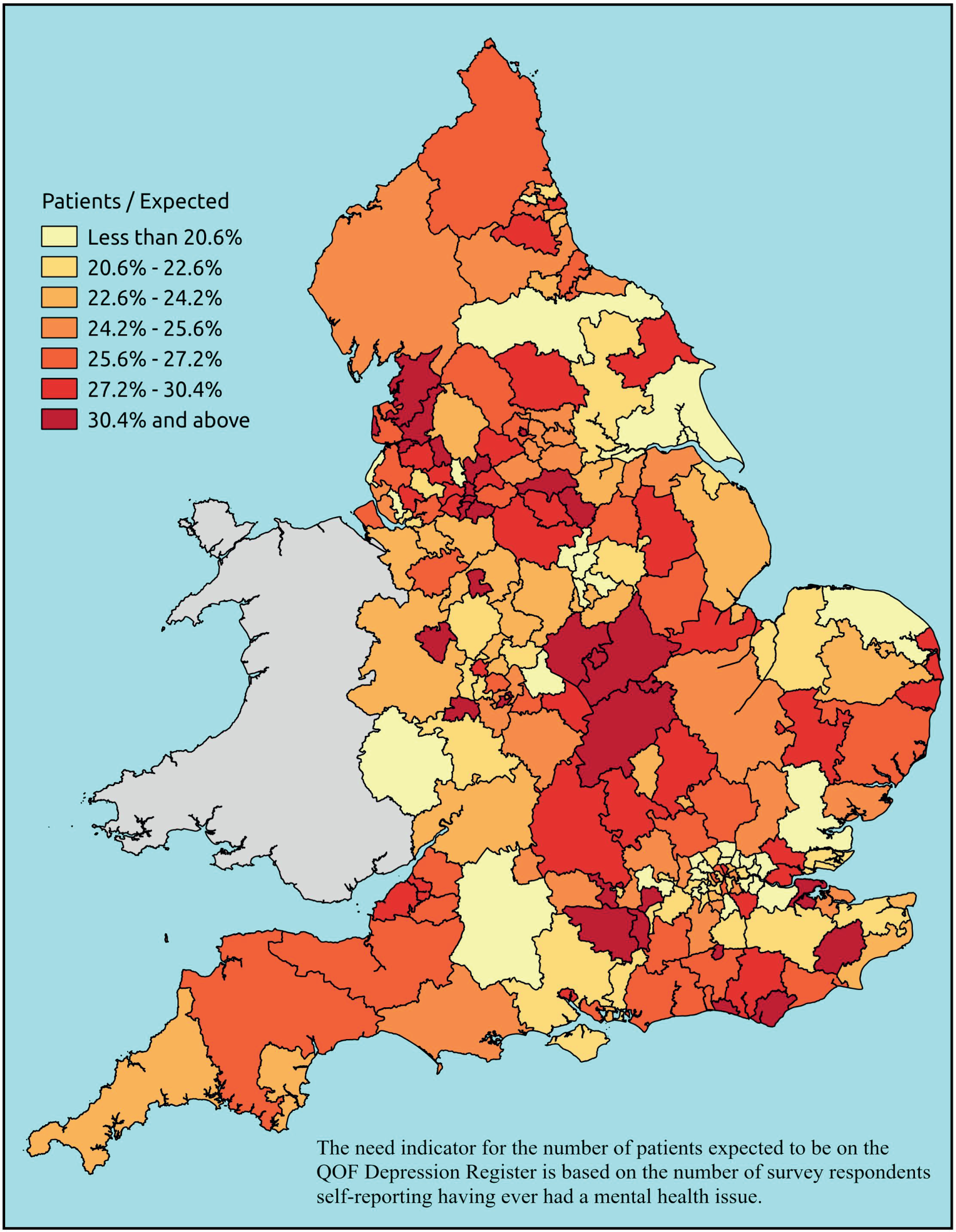
FIGURE 11.
Clinical Commissioning Group-level variations in NIC prescribing on hypnotics, anxiolytics and antidepressants489 per expected person who is ‘extremely anxious/depressed’. Contains Ordnance Survey data © Crown copyright and database right 2012.

FIGURE 12.
Clinical Commissioning Group-level variations in patients in contact with specialist community services158 per expected person who has ‘had a mental health issue in the last 12 months’. Contains Ordnance Survey data © Crown copyright and database right 2012.
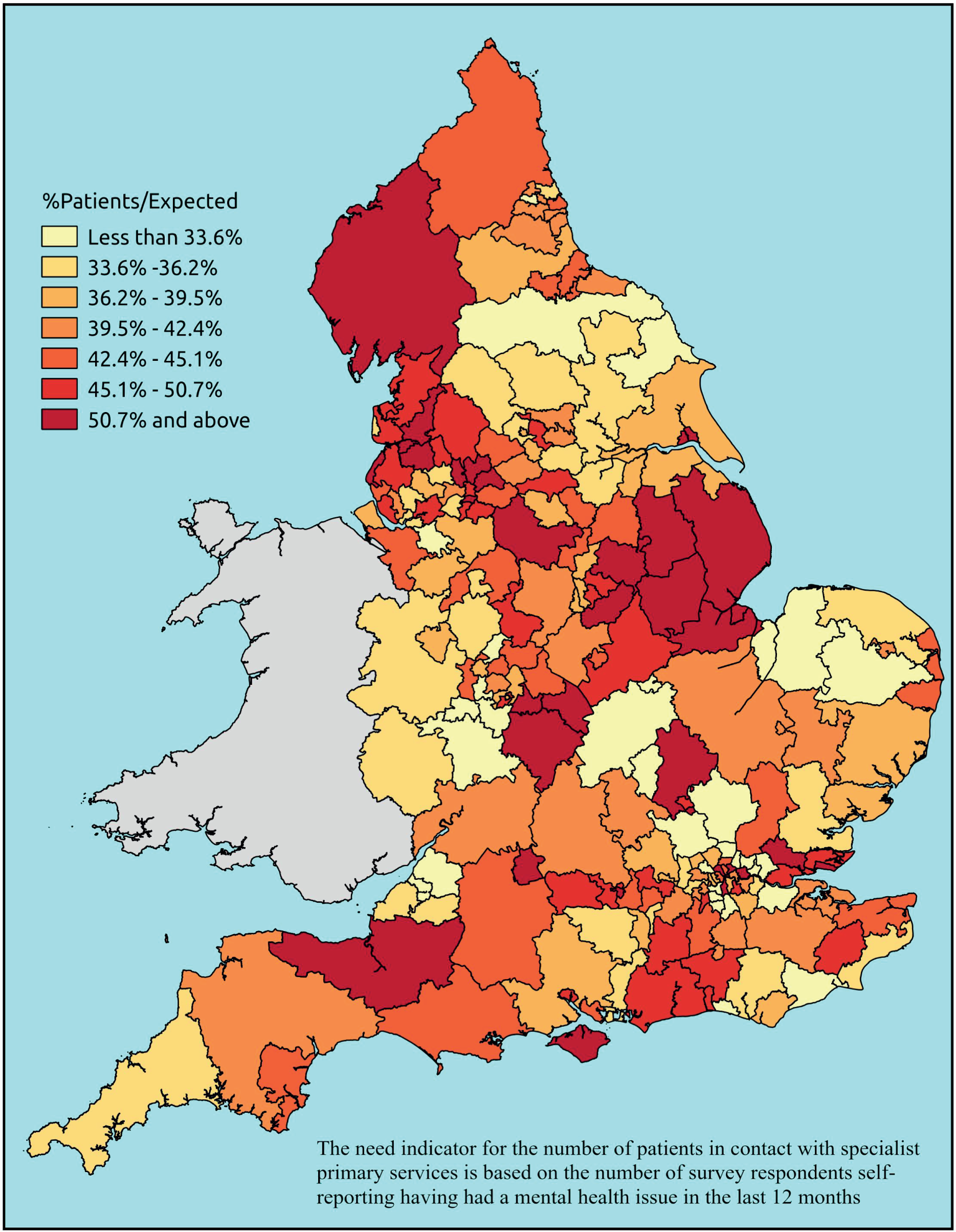
It appears there is strong evidence that in London, relative to national norms, utilisation of primary care and prescribing relative to need is much lower than might be expected, perhaps suggesting a local mental health service that is unable to adequately meet the primary care needs of its client population. In terms of the number of people accessing specialist community services, however, the overall London use-to-needs ratio is only slightly lower than the national average (38.7% as opposed to 41.2%) and, as illustrated by Figure 12, this includes considerable CCG-level diversity.
Beyond this London effect, it is difficult to point convincingly to any particular geographical tendency save that of great diversity. This is perhaps best illustrated by looking at the most local scale, namely how practice-level QOF Registration and prescribing rates vary relative to need (Figures 13 and 14, respectively). These maps are, of course, seriously compromised by the fact that they attempt to include information on nearly 8000 practices, but such notwithstanding, the degree of local variation is apparent. Even within London, where CCG-level QOF Registration and prescribing rates relative to need are almost invariably much lower than might be expected, there is still considerable practice-level diversity, though the generally lower level of QOF Registration and prescribing in the capital remains apparent.
FIGURE 13.
Practice-level variations in QOF depression registered patients440 per expected person ‘who has ever had a mental health issue’. Contains Ordnance Survey data © Crown copyright and database right 2012.
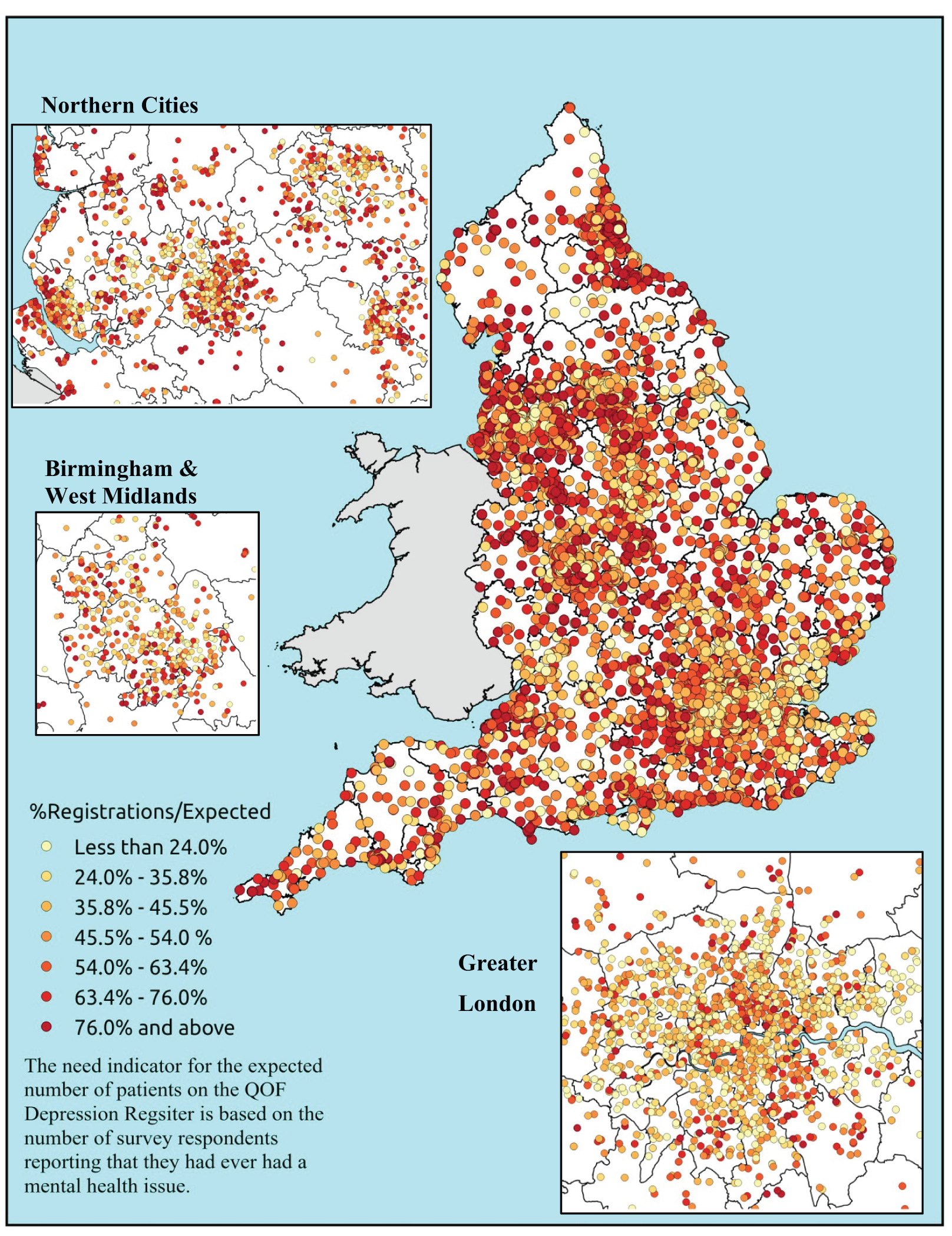
FIGURE 14.
Practice-level variations in NIC prescribing on hypnotics, anxiolytics and antidepressants489 per expected person who is ‘extremely anxious/depressed’. Contains Ordnance Survey data © Crown copyright and database right 2012.
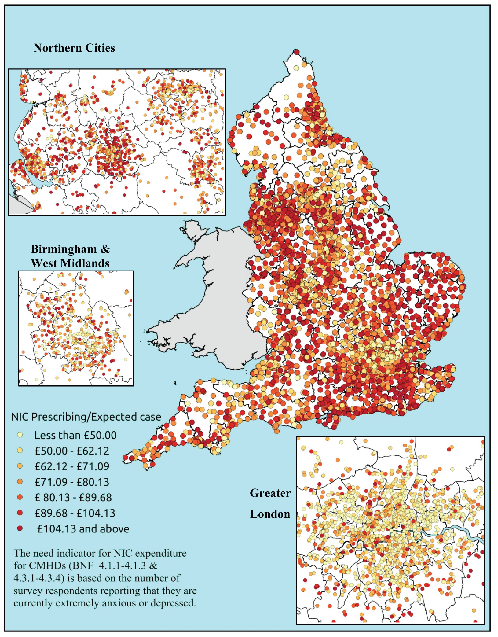
Thus, compared with patterns of use relative to need across the cardiovascular and related conditions considered in Chapter 4, the situation with respect to mental health is much more variable. It appears that there is a genuine ‘postcode lottery’, with access and uptake of services varying in ways that are only partly related to need and, save a possible serious underprovision of services relative to need in London, only marginally affected by the socioeconomic, demographic or geographical factors considered here. There may, of course, be very local (sub-CCG) organisational issues at work which we have, as yet, been unable to address.
Conclusion
If, as argued above, higher percentage R2 correlation coefficient values between per-capita needs and per-capita utilisation rates are indicative of a more ‘equitable’ use of health-care services relative to need, then it is of some concern that variation in mental health service use is poorly explained by underlying need. As the addition of potential explanatory factors does little to improve matters, the overall picture is one of unexplained variation.
Key findings
-
Rates of QOF registration and prescribing tend to be lower than expected in areas with large black populations.
-
Rates of QOF registration and prescribing tend to be higher than expected in areas serving more deprived populations.
-
Our findings of lower rates of mental health use among black populations and higher rates among deprived populations corresponds with existing literature. However, there is little evidence of inequality among older populations, which conflicts with a key finding of the literature review.
-
There appears to be a ‘London effect’, with rates of QOF prevalence and particularly prescribing being much lower than expected in London than in the country as a whole.
-
There is considerable practice-level variation in use relative to need, even within London and other major cities.
Chapter 6 Summary, conclusions and implications for policy and research
Introduction
The fact that this study has found little consistent evidence that deprived populations make lower than expected use of cardiovascular and mental health services may be surprising to those with an interest in health policy and health services research. The inverse care law has become a powerful meta-narrative in accounts of variations in access to and use of health care. Indeed, comments by senior NHS/Department of Health representatives, prominent medical commentators and politicians suggest that the idea that socioeconomically disadvantaged people are also disadvantaged in their access to health care is accepted by the mainstream. In the 2014 annual lecture to the Health Service Journal, Simon Stevens, Chief Executive of NHS England, referred to ‘some inner city areas where the inverse care law has persisted for years, you have an under-doctored area that is hard to recruit to, where perhaps there have been quality and access concerns’. 494 Iona Heath, ex-president of the RCGP, nominated by Pulse495 as the third most influential GP in the UK, has been passionate about the injustice of inverse care:
There is a desperate need to distribute health services resources according to need . . . Poorer people . . . need commensurately more access – not less as now . . . Why is Julian Tudor Hart’s inverse care law so pervasive even within the NHS . . .?496
Despite presiding over a significant redistribution of NHS resources towards deprived areas, the New Labour government also expressed concerns about inequity with respect to access to health care. Writing in 2006, Patricia Hewitt, the then Secretary of State for Health, claimed: ‘We’ve achieved a great deal, but there’s more to do. The “inverse care law”, whereby communities with the greatest health needs get the poorest services, still applies . . . Our White Paper will address these historic injustices’. 497 There are, however, few signs that professional bodies such as the RCGP believe that the injustice of inverse care has been addressed. As noted in Chapter 1, problems of access in deprived areas have been highlighted in several recent RCGP reports,101,102 with associated calls for GP funding to be more strongly weighted towards deprivation.
It is not only policy circles that accept the conventional wisdom of inverse care. In an editorial comment about research evidence on variations in health service use in Canada, Hutchison notes that some studies ‘show greater use of hospital services by those with lower income after controlling for healthcare need – perhaps calling into question the adequacy of existing measures of need’ (our emphasis). 498 This illustrates the ongoing tendency to believe that more intensive use of health services by lower income groups is always appropriate, and raises a wider issue with respect to research design and interpretation. As we proposed in Chapter 1, taken-for-granted assumptions can shape researchers’ choices about the way in which they pose research questions, design studies and interpret results or, in the case of editorial teams, make decisions about what to publish. Thus, if inequalities in access are to be properly understood and acted on, it is important that research is objective and robust.
Producing such evidence has been the aim of this project, a key rationale of which was our concern about the way in which the use of proxy measures for health service need may have given rise to findings that are subject to statistical artefact. Although, as we discuss below, it is important to examine ‘within-system’ inequalities in access to and utilisation of care, for example the extent to which particular hospital treatments and/or procedures are provided relative to the number of people admitted with a particular diagnosis, it is also important to acknowledge that such data will incorporate both unmet need and unjustified supply. In other words, they may bias our understanding of the extent to which services are being accessed relative to underlying need.
Against this background, we have sought to produce modelled estimates of health service need that are independent of unmet need and supply and to analyse those estimates against measures of health service utilisation. The focus on CVD and CMHD has allowed us to explore our hypothesis that the nature and direction of variations in access and use are likely to vary according to clinical conditions. Available data sets on utilisation (which are particularly rich with respect to CVD) have allowed us to examine whether or not variations in use relative to need differ at different points of the care pathway. Reflecting a concern that other dimensions of inequality may have been relatively neglected owing to a prevailing concern with inverse care, we have also explored the extent to which the ethnic, age and geographical characteristics of populations explain variations in use relative to underlying need.
Summary and discussion of findings
Estimating local disease prevalence
The decision to use a ‘bottom-up’ approach to estimating population-level disease prevalence through the aggregation of modelled individual-level disease risk estimates raised significant methodological and computational challenges. We were nevertheless concerned to produce estimates that were independent of issues of candidacy and adjudication. We have also sought to avoid a priori decisions about which particular survey questions (or biometric evidence) would best reflect variations in need and have instead made post-hoc assessments of the face-validity of the final estimates vis-à-vis a suboptimal but unavoidable comparison with available utilisation data. We have been clear about the fact that, in the absence of ‘gold-standard’ comparator data, confidence in the estimates must ultimately rest with the suitability and utility of the estimation methodology that underpins them. It is nevertheless encouraging that we were able to construct need estimates for CVD, diabetes, CHD, hypertension and stroke that are significantly better predictors of variations in QOF registration rates than the currently available PHE estimates. Furthermore, whereas the Plymouth estimates were generally incorporated as the most important factor in linear regression modelling of variations in health service utilisation, the PHE need estimates behaved erratically. We have little doubt that these new estimates offer a step-change improvement in our knowledge concerning the distribution of CVD and CVD-related needs.
The mental health estimates are more difficult to assess. Forty-one different estimates were produced, which give rise to a diversity of prevalence rates, not all of which even relate to each other. As predictors of QOF prevalence, they perform poorly. Indeed, in stark contrast to hypertension, CHD and diabetes, there is surprisingly little relationship between the proportion of patients on QOF Depression Registers and estimates of either (a) the number who report having ‘ever been diagnosed’ with depression or (b) any of a large number of self-reported or schedule-based assessments of the presence of a CMHD. For instance, at practice level, the strongest correlation with QOF registration rates is with the proportion of people who report that they ‘had ever had a mental health issue’ (R = 0.386; R2 = 0.149).
Prevalence rates based on established schedule-based assessments of the presence of CMHDs are even less well correlated with QOF registration rates. For instance, correlation with GP-level estimates of the proportion of people with a CIS-R score of ≥ 12 (commonly taken to indicate the presence of a non-psychotic psychiatric disorder) is R = 0.088 (R2 = 0.008), while correlation with the estimated proportion of people scoring ≥ 18 (indicative of a non-psychotic psychiatric disorder in need of treatment) is only marginally better at R = 0.121 (R2 = 0.015). The CIS-R interview captures a wide range of non-psychotic mental health disorders, but the subset concerned with ‘symptoms of a depressive episode’ generates a set of estimates which are only marginally better correlated with QOF Depression Register rates (r = 0.124; r2 = 0.015). Estimates of the proportion of people with a GHQ12 score of ≥ 4 (indicating possible psychological disturbance or mental ill health) are similarly poorly correlated with QOF rates (R = 0.134; R2 = 0.018).
The overwhelming impression is that our modelled estimates of the prevalence of depression (and non-psychotic mental illness generally) bear very little relation to QOF registration rates; but is this because of a complete failure of our approach to capture variations in CMHD morbidity, or because QOF registration of depression is profoundly variable?
In the first place, it would be surprising if the underlying approach, demonstrably effective with respect to hypertension, CHD and diabetes, should fail with respect to mental health. Thus, although it is possible that the way in which people respond to questions about their mental health may undermine the use of the resulting data for predictive purposes, the fact of the matter is that the same data sources are used, the same method of deriving individual-level risk estimates is employed, and those estimates are then applied to the same microsimulated populations. Second, some of the modelled estimates for CMHDs perform much more creditably with respect to other measures of health service use. For instance, in stark contrast to their lack of association with CCG-level QOF registration (R = −0.005), estimates of the proportion of adults with a CIS-R score of ≥ 12 are much better correlated with estimates of the proportion of adults in contact with secondary services (R = 0.570; R2 = 0.322). Similarly, although the proportion of adults reporting that they ‘had a mental health issue in the last 12 months’ is relatively poorly correlated with QOF registration rates at CCG-level (R = 0.379; R2 = 0.143), it is a better predictor of the proportion of adults accessing community mental health or IAPT services (R = 0.516; R2 = 0.263). CCG-level prescribing, meanwhile, correlates relatively well with CCG-level estimates of the proportion of adults per capita reporting ‘extreme anxiety and/or depression or taking prescribed mental health medication’ (R = 0.689; R2 = 0.472).
These associations are not as close as those found with respect to diabetes, hypertension and CHD, but they do indicate that the proportion of adults QOF registered with depression is likely to be a poor indicator of underlying rates of depression, let alone of non-psychotic mental illness more generally. In other words, much of the discontinuity between our estimates of need and QOF registration rates is likely to lie with practice- and PCT-/CCG-level variations in case finding.
One cannot, of course, attribute ‘truth’ to the modelled estimates of need and we recognise that the mental health estimates are, by their nature, more problematic than those for CVD. Indeed, given ongoing debate about the construct validity and reliability of psychiatric diagnostic categories and criteria (diagnosis itself purportedly lacking a gold standard), the hope of producing clear and uncontested indicators of mental health service need was perhaps naive. Yet there were some encouraging findings, not least the fact that the modelled prevalence rates were significantly more effective than both QOF prevalence and the existing Public Health Observatory estimate at predicting CCG-level variations in the number and proportion of people accessing community mental health and IAPT services, as well as at predicting variations in secondary mental health service use.
We thus argue that the Plymouth estimates are based on methodological rigour and offer useful measures of underlying need with respect to both CVD and CMHDs. They may not be definitive, but need estimates are required for planning, commissioning and evaluative purposes and, for the present, there is no plausible alternative means of quantifying the underlying ‘need’ for health-care services.
Understanding the distribution of health service need
To this end, an important finding is the significant variation that exists in the geographical distribution of CVD and CMHD. Reflecting the relative contributions of age, deprivation, ethnicity, etc. in disease risk, the prevalence of most CVD conditions is largely driven by demography and exacerbated by poverty. Thus, the highest prevalence rates of diabetes (a risk factor for CVD) are to be found in Lincolnshire, Newcastle and Tyneside, North Devon and Cornwall, areas in which older age profiles and deprivation combine to increase disease risk. Stroke and hypertension prevalence show similar patterns, although more coastal areas (with ageing demographies) show up on the maps of high prevalence. It is, however, important to note that not all CVD prevalence estimates are distributed in this way. For example, self-reporting a heart/circulatory disease as a self-reported LSI shows a distinct north (high)/south (lower) pattern.
Mental health, by contrast, has a strongly urban distribution. This is particularly the case when based on CIS-R ≥ 12 and ≥ 18 criteria, although most of the prevalence estimates show a similar pattern (although Lincolnshire also appears to be a high-prevalence area). Symptoms of a depressive episode slightly bucks this trend, with high rates being found in demographically older coastal areas such as Cornwall, Devon, Norfolk, Kent and, again, Lincolnshire.
The main conclusion to be drawn here is that the distribution of crude prevalence varies by clinical condition. Moreover, the pattern of CVD prevalence is not cognate with patterns of standardised morbidity and mortality which have been increasingly deployed as proxies for health service ‘need’. It is important that service planners and commissioners recognise this difference. As standardised rates effectively design out the effects of age, they are poor proxies for the crude prevalence of (and, by association, health service need for) diseases where risk is highly age-related. There is a need for greater clarity about the purpose and impact of age standardisation and we believe that our prevalence estimates and maps will make a contribution towards this end.
Existing literature on variations in access and use
As noted above, taken-for-granted assumptions can shape researchers’ choices about the way in which they pose research questions, design studies and interpret results. In our review of existing literature, we found that studies that had explored inequalities in access to and use of CVD care were more likely to have focused on socioeconomic status, while studies on access to/use of mental health services were more likely to have focused on ethnicity.
Study design can influence the eventual evidence base, though we note a distinct improvement in the methodological quality of studies since the 1990s. Accepting published literature at face value, reviewed studies suggest that older age and female sex are the key dimensions of inequality with respect to CVD care; and older age and non-white ethnicity are the key dimensions of inequality with respect to mental health services. For both CVD and mental health, very significant unexplained geographical variation exists in utilisation. Evidence of socioeconomic bias in access and/or utilisation is more ambiguous and contradictory.
The methodological quality of studies is better for CVD than for CMHD. Most accounts of mental health use do not adjust for underlying need, in part, no doubt, because of the hitherto lack of robust estimates of need.
Analysis of use relative to need
Relating use to stage on the care pathway
As noted in Chapter 1, we have proposed that the model of candidacy and adjudication provides a useful framework by which to understand that inequalities in use can arise at different stages of the care pathway. In order to access services, people need to recognise their eligibility as candidates for health care in the first place. Delay, denial, confusion about symptoms, embarrassment or a preference for self-management can influence decisions to seek help, as can practical issues such as the need to arrange childcare/time off work. Problems that arise before GPs become involved can be addressed through sensitive and targeted health service interventions (such as awareness campaigns and support for transport). However, they cannot be simply attributed to inequalities in health service availability.
Once patients have gained entry to the system, the categorisation and disposal of their health needs depends to some extent on their ability to present in ways that health professionals find credible and legitimate. In turn, the way in which health professionals categorise health needs may be affected by pre-existing attitudes, perceptions of patient preferences, technical eligibility and knowledge and/or experience of local capacity. These are important issues of concern from a policy perspective insofar as practitioner attitudes and health service capacity are within the remit of those deciding matters relating to professional practice, resource allocation and so on. In understanding the factors that shape clinicians’ decisions to open up the pathway to treatment, it is also important to note that there is not always a clearly cut boundary in the locus of decision-making. Thus, although GPs are usually responsible for initial referral to specialist care, it is the specialists themselves who determine access to secondary-level treatments.
As a large-scale, statistical investigation, we acknowledged from the outset that the study would not yield in-depth qualitative evidence of the ways in which candidacy is recognised and asserted, how people are categorised and disposed by health professionals, or of interactions between these processes. However, by potentially identifying systematic effects at different stages of the pathway to care, we did hope to gain insights into key points of candidacy and adjudication that would lend themselves to further quantitative and qualitative research.
Variations in disease presentation
For both CVD and CMHDs, we have sought to examine where inequalities arise at different stages of the care pathway. Using QOF registration as a measure of presentation is not an ideal method of capturing help-seeking behaviour, as it is an outcome of the decision by patients to access primary care, of GPs to make a diagnosis and, of course, of the proper maintenance of QOF registers. However, in view of the financial incentives associated with the QOF and evidence that, over time, variations in the achievement of QOF indicators have significantly declined (suggesting a greater consistency of recording and practice), we propose that QOF data are the best available measure of primary presentation.
The findings suggest that the level of unmet need (where modelled estimates exceed diagnosed prevalence) varies from condition to condition. We found that the overall number of patients estimated to have diabetes in the community (using different definitions) is very similar to the overall number of people on the QOF register. This may reflect the fact that this disease produces distinct symptoms (e.g. feeling very thirsty, passing more urine than usual, feeling tired all the time) that are likely to promote help-seeking behaviour. Diabetes is also a well-defined condition that is straightforward to diagnose. This is not to say that there is no inequality in the presentation and diagnosis of diabetes. In terms of the need indicator based on the number of people reporting diabetes as a LSI (the most effective estimate at predicting variations in QOF registrations), there is a 1.77-fold variation in PCT-level registrations per expected (modelled) case. Moreover, although registration is significantly higher than one might expect among Asian populations and in deprived and rural communities, it is significantly lower in practices with larger percentages of black populations. At PCT level, there is also some evidence to suggest that, relative to underlying need, younger populations are less likely to be diagnosed with diabetes. As noted above, this statistical analysis does not allow us to conclude whether variations in modelled versus diagnosed prevalence arise from demand- or supply-side factors. It nevertheless provides some pointers for future research and policy (see Implications for further research).
Hypertension is also a well-defined condition. However, in many cases, it has no symptoms that would lead people to consult their GP. Thus, while our needs estimate based on ‘clinical evidence’ of diagnosed or undiagnosed high blood pressure predicts 99.2% and 77.8% of the variation in QOF counts at PCT and practice levels, it also yields evidence of high levels of unmet need. The modelled prevalence rate (aged ≥ 16 years) of 32.3% greatly exceeds the QOF prevalence rate of 13.6%. This suggests underdiagnosis of 58% of expected cases, compared with 45% of expected cases in the 2011 NHS Atlas for Variation. In our study, there is a 1.53-fold variation in PCT-level registrations per expected (modelled) case, compared with a 1.7-fold variation in the NHS Atlas for Variation. Again, of the factors that yield significant standardised coefficients at the PCT and practice levels, underlying need accounts for most explainable variation in QOF registration. Smaller but significant coefficients are found for percentage black population and percentage population under 50 years, both of which are associated with higher presentation rates than expected. Presentation of hypertension in more rural PCTs and practices is significantly lower than expected, although again the coefficients are small. It is interesting to note that population characteristics associated with underdiagnosis vary between diabetes and hypertension, and tempting to suggest that whereas the former reflects individuals’ willingness to respond to specific symptoms, the latter may reflect the extent to which GPs proactively identify the presence of an often asymptomatic condition.
A number of modelled prevalence rates are available as potential ‘needs indicators’ for CHD. Using ‘clinical evidence of CHD’ as the basis on which to measure health service needs, we estimate a prevalence rate of 11.6% among those aged ≥ 16 years. This compares with the national QOF CHD prevalence rate of around 4.2% aged ≥ 16 years, again suggesting significant levels of underdiagnosis (64% of expected cases). The modelled prevalence rate of doctor-diagnosed CHD (5.4%) is far closer to QOF prevalence. However, we have questioned whether or not such an explicitly utilisation-based measure of needs should be used as the basis for assessing how use varies relative to need. Using the clinical evidence measure, there is a 2.37-fold variation in PCT-level registrations per expected cases (which compares with a 2.7-fold variation in the 2011 NHS Atlas of Variation). Modelling variations in use relative to need, we found that QOF registration is significantly higher than one might expect among Asian populations and significantly lower in PCTs with higher percentages of black and younger populations at both PCT and practice levels. We found no evidence of socioeconomic differences in QOF registration.
Although the number of people estimated to be living with stroke as a LSI condition is very strongly predictive of PCT-level variations in the number of people on the QOF register, the overall estimated prevalence (1.0%) is much lower than the overall QOF registration rate (1.7%). The prevalence estimate is, nevertheless, a good predictor (% R2 = 98.3%) of PCT-level variation in QOF counts and, thus, can be used to explore variations in the health-care use relative to underlying need. Here, we find a 1.63-fold variation in PCT-level registrations of stroke per expected cases and, although stroke registration and prescribing at the practice level of analysis are higher than expected in more deprived areas, younger age and ethnicity emerge as consistently significant coefficients of lower use. In this case, both black and Asian populations appear to have lower QOF registrations than expected.
Across all of the CVD and CVD-related conditions that we analysed, ethnicity emerged as a consistent predictor of variations in use relative to need. This possibility has received far less attention than that of socioeconomic variations in utilisation. We consider it to be an important finding, as is the evidence that patterns of use appear to vary between South Asian and black populations. There has been a tendency in the past to group different ethnic groups into one category. The results of this research suggest the need for a more nuanced approach and for further investigation into whether differences in help-seeking behaviour between different ethnic groups reflect cultural, economic or health service factors.
Turning to CMHDs, as noted above, the prevalence estimates were far less effective at predicting variations in QOF registrations. Even the best predictor, namely the proportion of adults who report that they ‘ever had a mental health issue’, explains only 30.4%, 37.2% and 14.9% of variation in QOF registration rates at CCG, PCT and practice level, respectively. Once additional factors describing key aspects of demography, ethnicity, deprivation and rurality are incorporated in a linear regression model, the proportion of variation in QOF registration that can be explained at CCG, PCT and practice level rises only to 35.3%, 42.9% and 17.0%, respectively.
A large proportion of the variation in QOF registrations thus remains unexplained at all levels, which may suggest the need for some caution in interpreting the findings. Thus, although it is plausible that, at local levels, the proportion of people being QOF registered fluctuates randomly, it is equally plausible that there are factors at work here that we have not been able to incorporate in this analysis. If so, then once included they may well affect the independent effect of factors such as deprivation and ethnicity. That said, our finding that areas with higher percentages of black populations have significantly lower QOF-recorded depression than expected does correspond with the results of many studies that find that being a member of an ethnic minority is associated with lower rates of help-seeking behaviour for mental distress. Again, however, the need for a more nuanced account is indicated. At practice (but not PCT/CCG) level, for example, we find that areas with higher percentages of Asian populations have significantly higher-than-expected rates of QOF registration. At all scales of analysis, more deprived areas have higher registrations than expected, which again corresponds to literature that suggests that the socially disadvantaged are more likely to seek formal help for mental health problems. In contrast to published literature, however, we found no evidence to suggest that younger or older populations have differential rates of diagnosis relative to need.
Variations in primary management
As one moves up the care pathway, the percentage of variance that can be explained by estimated prevalence tends to fall (particularly with respect to CVD and CVD-related conditions). The data that are available to us cannot explain the extent to which unexplained variation is legitimate (patients with ostensibly similar diagnoses requiring different levels of treatment) or stems from inappropriate processes of adjudication by clinical professionals. Nevertheless, we do find evidence of systematic variation, which raises concerns.
All of our measures of primary management relate to prescribing, which are measured by either rates of prescribing of specific BNF categories or PBC expenditure. With respect to diabetes, we find similar patterns to those relating to presentation of disease. Thus, rates of prescribing are significantly higher than expected among Asian populations and in deprived and rural communities, and lower in practices with larger percentages of black populations. With respect to the demography of communities, the results are mixed, with practices with a higher percentage of adults under the age of 50 years being less likely to prescribe diabetic drugs (BNF 6.1487) and other antidiabetic drugs (BNF 6.1.2487) but more likely to prescribe insulin (BNF 6.1.1487).
Prescribing data for CHD also suggest higher-than-expected rates of primary management among Asian populations and lower-than-expected rates among younger and black populations (although it is important to note that these additional factors explain a relatively small proportion of overall variance). Variations in prescribing according to deprivation and rurality are mixed according to type of medication, suggesting no overall pattern with respect to socioeconomic status and geography. By contrast, primary management of hypertension shows no clear pattern of ethnic variation, although rates of prescribing are higher than expected in deprived communities and lower than expected in rural areas.
Rates of prescribing for stroke (at the practice level) are also higher than expected in more deprived areas. In this case, however, younger age and ethnicity emerge as consistently significant coefficients of lower use. Black and Asian populations appear to have lower prescribing of oral anticoagulants and warfarin than expected. Antiplatelet prescribing is also lower than expected among black populations.
As noted above, the results on variations in use relative to need for CMHDs are more difficult to interpret. Nevertheless, ethnicity again emerges as a consistent predictor. At CCG, PCT and practice levels, the percentage of population that is ethnically black is an important predictor in the linear regression of variations of per-capita prescribing (with areas with higher proportions of black/black British populations having lower-than-expected rates of prescribing). This corresponds with evidence from the National Psychiatric Morbidity Surveys. Reviewed evidence also suggests that prescribing for anxiety and depression is significantly lower in areas with higher percentages of Asians, which corresponds to our findings at CCG and practice levels. Levels of prescribing are significantly higher than expected in more deprived CCGs, PCTs and practices. Again, this tallies with the conclusion of published studies that find no evidence of inverse care in the treatment of moderate and severe depression. Unlike the published literature, we find no evidence of systematic undertreatment of older populations. We do, however, note the presence of, and possible wider consequences of, a ‘London effect’, where prescribing relative to need appears to be much lower than might be expected.
Variations in specialist management
Investigation of variations in use relative to need of specialist services provides some intriguing insights into the role of the relative mix of care, particularly for diabetes. PCTs and practices with a higher percentage of Asian populations have lower-than-expected rates of admission (elective and emergency) for a main diagnosis of diabetes and lower PBC expenditure on the disease. By contrast, PCTs with a higher percentage of black populations have higher PBC expenditure on hospital care (data available at PCT level only). This suggests the possibility that, among Asian populations, diabetes may be better managed within primary and community settings than it is among other population groups. Against this, more deprived PCTs and practices have higher-than-expected rates of both prescribing and secondary care (particularly with respect to emergency admission for diabetes as a main diagnosis), and PCTs and practices with higher black populations have lower utilisation rates than expected in both primary and secondary care.
With respect to the secondary management of CHD, the percentage of variance explained by both underlying ‘need only’ and ‘full model’ falls away significantly. This is likely to reflect the fact that ‘within-system’ management is a more important determinant of need for specialist CHD services than underlying prevalence. Effective management within primary and community settings means that a good proportion of patients with CHD can avoid hospital intervention. The fact that significantly higher rates of CHD presentation and prescribing among South Asian populations are not accompanied by lower rates of inpatient use does not necessarily undermine this argument. Given evidence that South Asians are at excess risk of CHD for reasons that cannot be explained by conventional risk factors, and that they tend to develop the condition at younger ages,477,478,491,493 their higher use of secondary interventions may well reflect the challenges of developing optimal prevention regimes for this population. It is, nevertheless, the case that the ‘relative mix’ explanation does not apply in other cases, such as that of stroke, for which black populations have lower QOF registrations, lower prescribing of oral anticoagulants and warfarin and lower secondary use than expected.
In addition to the role played by relative mix, we note that there may be regional variations in access relative to need which cannot be explained by compositional (i.e. socioeconomic, sociodemographic and ethnic) characteristics. For instance, the North East has relatively high levels of secondary expenditure on cardiac care, as do parts of the South East and South Central regions. By contrast, ‘Shire England’ has relatively low rates of secondary expenditure relative to need. It also has lower levels of prescribing, which suggests that relative mix of care does not fully explain the pattern. There are a number of possible explanations for this, of which we consider the funding context to deserve further investigation.
Turning to the specialist management of CMHDs, we find no evidence of systematic bias – by socioeconomic status, age, ethnicity or rurality – in rates of IAPT uptake relative to need. In that sense this would appear to be an equitable service, although there are geographical differences in service availability which may reflect factors that have not been included in the linear regression model. There is also little evidence that the number of people in contact with secondary mental health services varies according to population characteristics at the CCG level, although, at the PCT level, areas serving more deprived communities are spending significantly less than expected. Thus, we find an interesting contrast between CVD and CMHD: although underlying prevalence appears to be a better predictor of need for more specialist CMHD services, the opposite appears to be true for CVD. Here, the estimates are better at predicting variations in presentation and primary care than hospital care. Differences in the relative effectiveness of primary care services to reach people with needs (poor with respect to mental health needs but much more equitably with respect to CVD and CVD-related conditions) may be part of the explanation, as may differences in patterns of disease severity (e.g. by age) and the effectiveness of primary management. Further work certainly needs to be done to examine variations in utilisation within age cohorts.
Strengths and limitations
A key strength of the research project lies in its practical contribution. We aimed to support service planning and delivery by disseminating, via PHE, estimates of CVD and CMHD health-care need at different spatial scales. We have succeeded in this aim by (a) providing PHE with a range of Plymouth needs estimates (for 24 CVD and CVD-related and 41 CMHD potential ‘markers of health-care need’) and (b) making these available at a range of geographical levels (LSOAs, MSOAs, upper- and lower-tier LAs, regions, general practices, PCTs, CCGs and SHAs). The latter point is important if constituencies outside the NHS are to make use of the prevalence estimates, supporting, for example, key public health functions that have now transferred to LAs. This approach also supports data linkage, which is particularly important, as indicators of health and health service utilisation against which needs estimates might be compared are made available for a range of different organisational and spatial units.
We have also demonstrated the consequences of using different measures of need in studies of health-care equity. The fact of the matter is that any shortcomings in the data and/or methods used to generate need estimates will result in spurious conclusions regarding health-care equity. For instance, if an estimate fails to fully capture the extent to which socioeconomic deprivation affects the prevalence of a particular condition, then, even if different populations make genuinely equitable use of health services, analyses based on that estimate will make it appear as if deprived communities are making greater use of health services than might otherwise have been expected. Establishing robust denominators of need is demonstrably sine qua non for any study of health-care equity.
This project has also served to demonstrate that needs estimation is perhaps more difficult than has been generally recognised. Certainly we found that constructing the needs estimates detailed in this report raised many more methodological and computational challenges than we had anticipated. We are satisfied that we offer a step-change improvement in prevalence estimates for a variety of specific CVD, CVD-related and mental health conditions, but we recognise that not all methodological issues have been fully addressed (see Implications for further research). We also hope that our pedantic exploration of the wide range of possible needs indicators (detailed in Appendices 26 and 27), and, in the main report, of the range of assumptions that underpin the construction of the various prevalence estimates, serves to emphasise the essentially contested nature of all needs estimates. Few studies of health-care equity pay sufficient attention to the appropriateness of their particular needs denominator, or to the extent to which its use may influence conclusions regarding patterns of health-care equity.
As a direct result of having to direct a very significant proportion of our research effort at developing a robust, if not yet definitive, methodology for generating prevalence estimates at a variety of scales and across a range of conditions, our ability to model demand- and supply-side factors influencing variations in use relative to need has been constrained. This part of the project has been far less ambitious than originally envisaged and, as detailed in Implications for further research, further research is needed to add value to the wealth of data generated by this project.
While this clearly means we have been unable, as intended, to explore specific issues such as the potential impact of service configuration and funding on health-care equity, it also means that our conclusions, particularly with respect to mental health, regarding relationships (or lack of relationships) between use-to-need ratios and sociodemographic factors must be treated with some caution. For instance, in the case of mental health, the overall picture presented here is one of unexplained variation, particularly with respect to the use of primary care services. This is an interesting and important finding because it hints at local variations in medical practice that threaten the principle of equal access to equal needs. It is thus clearly necessary, as noted in Implications for further research, to extend the analysis of variations in use relative to need to include additional demand- and supply-side factors. In other words, further analysis may show there to be significantly less unexplained variation in the use of primary mental health-care services than currently appears to be the case.
Furthermore, until this further analysis is undertaken, it is not possible to entirely discount the possibility that our current understanding of the role that demography, sex, ethnicity and deprivation play in determining variations in use relative to need will change. For instance, the current analysis suggests that, at GP level, relatively little variation in the use of primary care services for CMHDs can be explained by variations in underlying need. The ‘full’ model, which incorporates ethnicity but ‘rejects’ the potential contribution of demography, deprivation and rurality, is only marginally better. With substantial unexplained residual variance, it is entirely plausible that further analysis will show supply-side factors to play a significant role in determining variations in health service use relative to need. Indeed, as noted below, this is an obvious and urgent issue to investigate. But, the fact is that, once such factors are allowed for, it is possible that the significance (or lack thereof) currently ascribed to demography, ethnicity, deprivation and rurality will change. This is important, for any policy response to inequalities in health care must be based on a convincing understanding of the underlying dimensions of those inequalities. With respect to diabetes, hypertension, CHD and stroke, this requirement has been largely met, although we do not discount the possibility that supply-side factors have a part to play. We are not convinced that the same can yet be said for our understanding of the determinants of the use of mental health services.
Finally, we are aware of the limitations associated with this study as an ecological analysis. Throughout, we have sought to describe observed relationships in terms of differences between populations. Thus, GPs with a higher proportion of Asian patients have higher QOF diabetes and CHD registration rates than might be expected, while GPs with a higher proportion of ethnically black patients tend to have lower QOF diabetes and CHD registration rates. This is, we believe, strongly indicative that, relative to need, Asian patients with these conditions are, individually, more likely to present to GPs and black patients are less likely, but one must always recognise that our perspective is ecological rather than individual. In this respect we are particularly concerned about the disconnect between our finding – that areas with older populations are neither less nor more likely to use services than expected – and the results of the literature search, which suggest that older age is a key dimension of inequality in access to/use of both CVD and CMHD care. In general terms it is clearly necessary to explore the observed ecological relationships to establish whether or not they reflect individual-level processes of candidacy and adjudication: in other words, taking this large-scale quantitative study as the starting point for more detailed, possibly qualitative, studies of how different individuals interact with health-care services.
Policy implications
As we noted in Chapter 1, policy-makers appear to have accepted the conventional wisdom of inverse care. Having positively targeted funding for hospital and community services at deprived areas, there are signs that GP funding may also be redistributed to better respond to deprivation. Yet, as this research shows, a GP managing a high caseload of one condition may have a lower caseload of another. We find that the geographical distributions of CVD and CMHDs are very different. CVD is higher in demographically older areas, particularly deprived coastal towns. By contrast, the highest prevalence rates of CMHD appear to be in major cities. Thus, although further targeting GP funding at deprivation will address ‘deep-end’ problems of managing mental distress, it will take funding away from practices that are managing high caseloads of degenerative chronic disease. There is an urgent need to establish the relative burden that these and other conditions place on GPs, as ‘robbing Peter to pay Paul’ will not promote equality of access for equal needs across the disease spectrum.
It is not, however, simply a question of understanding the relative burden that these conditions place on GPs; it is also a matter of establishing the relative importance that the public believes should be attached to these, and other, conditions. Thus, we also noted in Chapter 1 that in recent years the pendulum has swung from support for horizontal equity towards the promotion of equality in terms of health outcomes. Health economists have argued that this is supported by the public, with studies of public preferences showing that there is a concern to reduce inequalities in health. Yet there is, inevitably, a problem in the way in which preferences are framed. 41 Although several studies have offered respondents an explicit choice between maximising population health and reducing inequalities in health,37,42 these trade-offs are described in general terms. This research offers the possibility of providing the public with explicit evidence-based choices, specifically about the consequences of prioritising mental health problems over chronic diseases such as CVD.
We note that ethnicity is a consistent predictor of variations in use relative to need, with areas with high proportions of black populations having lower rates of use than expected. This is pronounced with respect to variations in presentation of CVD and CMHDs, suggesting that efforts could usefully be targeted at raising awareness, strengthening screening activity and so on in these areas and with respect to these populations.
Finally, given that this project has made available detailed data on the prevalence of CVD, CVD-related and mental health conditions at a variety of organisational and spatial scales, commissioners (at both national and CCG level) should be encouraged to utilise this information when making decisions regarding service provision (including service configuration and funding).
Implications for further research
As noted above, a substantial proportion of our research effort was absorbed by the methodological and technical challenges faced when seeking to generate robust prevalence estimates. The resulting estimates offer a step-change improvement on what has hitherto been available with respect to CVD, CVD-related and mental health conditions, but we recognise that not all methodological issues have been fully addressed. Insofar as we also demonstrate that suboptimal needs denominators can seriously contaminate health-care equity analyses, possibly removing or reversing the significance of individual factors, an obvious and important area for further research must be to consider further those specific methodological issues about which we have continuing concerns.
Enhancing prevalence estimation and exploiting the prevalence estimates
The final prevalence estimates rest on a proper understanding of the detailed sociodemographic composition of local populations, and this was established through microsimulation. Four issues arise with respect to microsimulation.
First, the ONS has recently published microdata for the 2011 census and these could significantly improve the iterative process which reconciles the aggregate characteristics of LSOA populations detailed in individual census tables to derive a description of the underlying, but unknown, ‘full joint distribution’ (see Chapter 3, Microsimulation for small-area estimation). As the microdata detail which of the myriad of theoretically possible person-types actually occur (albeit within a 10% sample), this would constrain the iterative allocation of individuals to cells so that cells known to be empty are not populated.
Second, microsimulation could be designed to reconcile tables across geographic levels (rather than just at LSOA level, as undertaken here). Census tables for higher geographies tend to be more precise (e.g. including all five general health categories in cross-tabulations rather than the three aggregated categories commonly used at LSOA level). The simultaneous iterative allocation of individuals to cells at multiple levels would add considerable computational burden, but this would ensure that the final microsimulation fits with a considerably wider evidence base. In a similar vein, the ONS will produce commissioned non-disclosive census tables (for a fee). A judicious choice of bespoke cross-tabulations at LSOA level or above could be used to further widen the range of ‘marginal distribution’ totals with which the final ‘full joint distribution’ would have to be reconciled.
Third, as noted in Chapter 3 (see Microsimulation for small-area estimation), in theory multiple solutions (i.e. full joint distributions) could meet the constraints defined by any given set of marginal distributions. It is intuitively likely that these will occupy a relatively small area within the multidimensional space defined by the marginal distributions (i.e. by the census cross-tabulation tables), but this is an issue we have not been able to explore in detail. Of particular concern is whether or not a variety of quite disparate solutions exist, and whether or not the solution to which the iterative ‘random walk’ method converges depends on its starting point. There is a need, in other words, to explore whether or not uncertainty surrounding the microsimulation of local populations is significant and, if so, whether or not that should be incorporated in the uncertainty surrounding the final prevalence estimates.
Finally, and more generally, a detailed description of the composition of local areas would be of value across many areas of research and planning. Implementing and disseminating (via a suitable web tool) a microsimulation covering all of the major sociodemographic variables, and reconciling a wide range of census cross-tabulations, could add significant value to the census. Care would be needed to ensure non-disclosure, but, given the methodology, this should not be an issue. The potential insights and utility of microsimulation is of growing interest, as recently summarised by Tanton and Edwards,499 and the experience of this project suggests that developing a web-based microsimulation tool would both be possible (if computationally demanding) and, if accompanied by an appropriate quantification of uncertainty, provide an invaluable resource to any analyses which need to use data on the detailed composition of local areas.
Turning to the modelling of survey data in order to estimate the likelihood that different individuals will exhibit or develop particular diseases, we are conscious that a number of essentially pragmatic decisions were made at various points. For instance, we decided not to request ‘special access’ survey data with additional information about precisely where individual respondents lived. This was partly because of the administrative difficulties and additional time involved, but primarily because, a priori, we decided not to utilise mixed-methods models. The problem, as we saw it, was that incorporating place (e.g. LSOA of residence) as a random effect in a mixed-effects model of needs risks introducing potential supply-side factors. Thus, if where you live influences how readily you can access a GP, and access to a GP influences the likelihood of being diagnosed with a condition (or, having been diagnosed, of reporting such as a long-standing illness), then using place of residence as a random effect in a mixed-effects model would, inevitably, incorporate this supply-side factor in the needs estimate. As a result it would most probably not appear as a relevant factor when variations in health service use are compared with the needs estimate. The point, however, is that the practical consequence of this, and the various other a priori decisions noted in Chapter 3, should be explored further in order to establish the sensitivity of the final estimates to those decisions. If the Plymouth estimates describing variations in the prevalence of CVD, CVD-related and mental health are to be as widely used by researchers, commissioners and public health practitioners as we believe they deserve, a thorough sensitivity analysis is possibly necessary.
Although, as detailed above, further research could be usefully directed towards the further improvement and evaluation of the methodology, more notable areas for further research concern the opportunities that arise now we have demonstrated that small-area estimation and microsimulation can be combined to generate robust prevalence estimates. First is a simple extension of the approach to cover a wider range of conditions. The various surveys used here, and particularly the HSfE, provide a wealth of evidence across a wide range of diseases. Indeed, the extent to which self-reported long-standing health problems predict variations in the use of health-care services for diabetes, hypertension, CHD and stroke is particularly encouraging, given that self-reported LSI data are widely collected using a standard reporting framework (Box 1). The methodology is perhaps not suited (or the results are maybe not useful) across all disease areas, but there is clearly considerable scope for extending the range of conditions for which prevalence estimates are produced and disseminated. In addition to that, of course, are a variety of doctor-diagnosed, biometric and other survey-based sources of information which could be used to provide a far broader understanding of how disease prevalence varies at various scales.
-
Cancer.
-
Diabetes.
-
Other endocrine and metabolic diseases.
-
Mental illness, anxiety, depression nerves.
-
Mental handicap.
-
Epilepsy, fits and convulsions.
-
Migraine and headaches.
-
Other problems of the nervous system.
-
Cataract, poor eyesight and blindness.
-
Other eye complaints.
-
Poor hearing and deafness.
-
Tinnitus and noises in the ear.
-
Meniere’s disease and ear complaints causing balance problems.
-
Other ear complaints.
-
Stroke, cerebral haemorrhage and cerebral thrombosis.
-
Heart attack and angina.
-
Hypertension, high blood pressure and blood pressure problems.
-
Other heart problems.
-
Piles and haemorrhoids, including varicose veins in the anus.
-
Varicose veins and phlebitis in lower extremities.
-
Other blood vessels and embolic conditions.
-
Bronchitis and emphysema.
-
Asthma.
-
Hay fever.
-
Other respiratory complaints.
-
Stomach ulcer, abdominal hernia and rupture.
-
Other digestive complaints.
-
Complaints of bowel and colon.
-
Complaints of teeth, mouth and tongue.
-
Kidney complaints.
-
Urinary tract infection.
-
Other bladder problems and incontinence.
-
Reproductive system disorders.
-
Arthritis, rheumatism and fibrositis.
-
Back problems, slipped disc and spine/neck problems.
-
Other problems of bones, joints and muscles.
-
Infectious and parasitic disease.
-
Disorders of blood and blood-forming organs and immunity disorders.
-
Skin complaints.
-
Other complaints.
A second obvious use of the methodology would be to focus on risk factors. Responding to interest expressed by colleagues in PHE, we used the Framingham Risk Calculator in conjunction with data from the HSfE to produce estimates of the number and proportion of adults aged 25–74 years (a) with a > 10% risk of developing CHD in the next 10 years, and (b) who would be expected to develop CHD in the next 10 years. We also produced prevalence estimates of the number and proportion of adults with three or more of NICE’s five modifiable risk factors for CVD. Although detailed in Appendix 26, these have not been discussed in the main report as they were peripheral to our main focus. Yet they are indicative of the wider range of risk factors and health-risking behaviours, such as smoking, obesity and physical inactivity, for which prevalence estimates could be produced. Although in many cases similar estimates already exist,441 these are not always available at sub-LA level, are seldom based on recent data and rarely use methods comparable with that developed as part of this study. Extending the current methodology to cover such risk factors would, we believe, significantly strengthen the public health evidence base.
A third important avenue for future research would be to address, head-on, precisely what the prevalence of particular diseases might mean in terms of health-care needs. There are two issues here. First, what health-care resources are actually used by individuals with specific self-reported, doctor-diagnosed or biometrically assessed conditions? Second, to what extent is that resource use sociodemographically invariant? Understanding these issues would be of particular interest to commissioners/planners of local health-care services as well as to those responsible for the allocation of resources to CCGs and general practices. For instance, it was noted above that although the further targeting of funding towards GPs serving more deprived communities might help them to address the high level of mental distress that is characteristic of such populations, in a zero-sum resource environment this would mean taking funding away from practices serving less-disadvantaged, but older, populations. These practices are typically managing higher caseloads of degenerative chronic disease. Establishing the prevalence of different diseases in different practice populations, as we have done for mental health and CVD, takes us only part of the way towards finding an equitable balance between these conflicting demands. What is also needed is an understanding of the demands such patients typically make on various health-care services, and to that end the recent linkage of HSfE respondents to HES data offers exciting new opportunities. Although individuals’ responses to HSfE questions were unavailable when we undertook this project, it is now possible to compare these with their use of inpatient, outpatient and accident and emergency services both before and after they were surveyed. As this can be quantified using, for example, reference costs, this means there is an opportunity to (a) investigate whether or not different types of person with any given prevalence marker for various diseases or conditions (such as a self-reported LSI) make different demands on NHS secondary services, and (b) utilise that information to translate cohort-level prevalence counts into explicit resource need estimates which, crucially and uniquely, are independent of supply-side influences.
This concern with how ‘raw’ prevalence counts relate to actual resource needs, and the extent to which such might vary by age and/or socioeconomic factors, could also be addressed by focusing on comorbidity and, where possible, symptom severity. Here the aim would be to replace models predicting the likelihood that different person-types would have, say, CHD, with more nuanced models predicting the likelihood that their CHD was accompanied by more or less complex health-care needs, which would primarily reflect the extent to which their CHD was accompanied by other health problems. Although it would be difficult to express such information in terms of actual costs, the aim would again be to provide local and national commissioners with unbiased evidence on the relative needs of different populations. Determining an equitable allocation of resources between very different populations – as illustrated above in terms of the conflicting needs of young urban deprived populations with relatively high rates of mental illness as opposed to less-deprived but older populations suffering high rates of chronic degenerative disease – requires a far better evidence base than is currently available. This project’s approach to estimating the prevalence of health-care needs in local areas suggests how this evidence base might be constructed and, by incorporating HSfE-HES linkage and/or evidence on comorbidity, could be developed to provide the information needed for the equitable allocation of NHS resources to CCGs and below.
Further research into health-care equity
We have not been able to investigate all potential demand- and supply-side factors and the impact they may have on the utilisation of health-care services. As discussed at length in Strengths and limitations, this means that many of our findings, particularly with respect to mental health, must be treated as provisional. The problem is that very little of the substantial GP- and PCT-/CCG-level variation in mental health service use (relative to need) can be explained with reference to demography, ethnicity, deprivation or rurality. Other factors may, or may not, be influencing the utilisation of primary and secondary mental health services, but, until their role has been fully investigated, our conclusions regarding the significance, size and even direction of the sociodemographic factors that have been considered must be considered provisional. This, then, is our single most important recommendation for further research and, as such, it is where our own future research plans focus. The fact of the matter, though, is that as the Plymouth estimates will be publicly available, this is an issue which other researchers can also readily address. Indeed, we hope that the availability of these estimates will encourage others to investigate issues surrounding health-care equity in England, particularly with respect to mental health, for which evidence on local variations in needs has hitherto been available.
Finally, this project has made genuine progress in identifying factors which are associated with variations in health service use relative to need. Summary and discussion of findings summarises many of the principal findings. However, as this is a large-scale ecological study investigating relationships between modelled estimates of need and health service utilisation data, it has not been possible to investigate the underlying processes which give rise to observed variations in health service use. As any policy response to inequalities in the use of CVD and mental health services requires a detailed understanding of why they arise, it is now clearly necessary to take the findings reported here as a starting point for a detailed investigation of individual-level processes of candidacy and adjudication.
Acknowledgements
Thanks are due to many people who have supported this project, not least Dr Richard Ayres, Dr Richard Byng and Dr Ian Mackenzie, who both provided clinical advice with respect to the ways in which appropriate clinical interventions linked to estimates of underlying need and have also read, commented and provided invaluable ‘on the ground’ perspectives on the report. Thanks are also due to Dr Julian Flowers, who has facilitated the application of our needs estimates for wider use via PHE.
We would also like to thank the Health Services and Delivery Research (National Institute for Health Research) team, in particular Donna White, for bearing with us in what has proved to be a very challenging project. The Health Services and Delivery Research team has been both flexible and accommodating in the light of very difficult personal circumstances. At the same time, the team has been rigorous with respect to its responsibilities with respect to monitoring project progress and outcomes, and has been gracious and proportionate. We hope that the final outcome of the report goes some way towards making up for the additional work that we have incurred.
Finally, acknowledgement is due to the providers of a number of key data sets.
Administrative data lookup products: supplied under the Open Government Licence. Contains Ordnance Survey data © Crown copyright and database right 2012.
Attribution Data Set: counts of the number of individuals in each unique non-null combination of MSOA, practice, sex, banded age (to match census quinquennial age bands) and whether or not the individual is in a nursing home. Provided by the Department of Health under Data Sharing Agreement DHADS2011003.
2011 census data: ONS, 2011 census: aggregate data (England and Wales) [computer file]. UK Data Service Census Support. Downloaded from http://infuse. mimas.ac.uk. This information is licensed under the terms of the Open Government Licence (www.nationalarchives.gov.uk/doc/open-government-licence/version/2).
Census Boundary Data: ONS, 2011 census: digitised boundary data (England and Wales) [computer file]. UK Data Service Census Support. Downloaded from http://edina.ac.uk/census.
Digital boundaries: digital boundary products and reference maps are supplied under the Open Government Licence and Ordnance Survey OpenData Licence. Contains National Statistics data © Crown copyright and database right 2012.
Hospital Episode Statistics data: pseudonymised Hospital Episode Statistics data containing all records extracted from the Admitted Patient Care data sets for 2009–10 to 2011–12. Copyright © 2013, reused with the permission of the Health and Social Care Information Centre. All rights reserved.
Contributions of authors
Sheena Asthana conceived and developed the research questions and protocol, led the project, carried out the literature review, advised on analysis and interpretation of results, drafted Chapters 1, 2 and 6, co-drafted Chapters 4 and 5 and, with Alex Gibson, collated and revised the final report.
Alex Gibson developed the research questions and protocol, managed the project, collected the data, developed the Plymouth estimates, carried out the analysis of use relative to need, drafted Chapter 3, co-drafted Chapters 4 and 5 and, with Sheena Asthana, collated and revised the final report.
Trevor Bailey contributed to the development of the Plymouth estimates and provided further advice on statistical methods and the analysis and interpretation of results.
Graham Moon contributed to the development of the research questions and protocol, advised on the analysis and interpretation of results and commented on draft chapters and the final report.
Paul Hewson contributed to the development of the Plymouth estimates and provided further advice on statistical methods and the analysis and interpretation of results.
Chris Dibben contributed to the development of the research questions and protocol and commented on draft chapters and the final report.
Data sharing statement
With regard to data access, data from this report can be obtained from Sheena Asthana (sasthana@plymouth.ac.uk).
Disclaimers
This report presents independent research funded by the National Institute for Health Research (NIHR). The views and opinions expressed by authors in this publication are those of the authors and do not necessarily reflect those of the NHS, the NIHR, NETSCC, the HS&DR programme or the Department of Health. If there are verbatim quotations included in this publication the views and opinions expressed by the interviewees are those of the interviewees and do not necessarily reflect those of the authors, those of the NHS, the NIHR, NETSCC, the HS&DR programme or the Department of Health.
References
- Tudor Hart J. The inverse care law. Lancet 1971;696:405-12. http://dx.doi.org/10.1016/S0140-6736(71)92410-X.
- Inequalities in Access to Cardiac Services: A Scoping Review. York: University of York; 2003.
- Dixon-Woods M, Kirk D, Agarwal S, Annandale E, Arthur T, Harvey J, et al. Vulnerable Groups and Access to Health Care: A Critical Interpretive Review 2005. www.netscc.ac.uk/hsdr/files/project/SDO_FR_08-1210-025_V01.pdf (accessed 7 January 2015).
- Greenhalgh T, Wong G, Westhorp G, Pawson R. Protocol – realist and meta-narrative evidence synthesis: evolving standards (RAMESES). BMC Med Res Methodol 2011;11. http://dx.doi.org/10.1186/1471-2288-11-115.
- Mooney G. Equity in health care: confronting the confusion. Effective Health Care 1983;1:179-85.
- Culyer AJ, Wagstaff A. Equity and equality in health and health care. J Health Econ 1993;12:431-57. http://dx.doi.org/10.1016/0167-6296(93)90004-X.
- Culyer AJ. The normative economics of health care finance and provision. Oxf Rev Econ Policy 1989;5:34-56. http://dx.doi.org/10.1093/oxrep/5.1.34.
- Culyer AJ. Equity – some theory and its policy implications. J Med Ethics 2001;27:275-83. http://dx.doi.org/10.1136/jme.27.4.275.
- Williams A. Intergenerational equity: an exploration of the ‘fair innings’ argument. Health Econ 1997;6:117-32. http://dx.doi.org/10.1002/(SICI)1099-1050(199703)6:2<117::AID-HEC256>3.0.CO;2-B.
- Culyer AJ. The bogus conflict between efficiency and equity. Health Econ 2006;15:1155-8. http://dx.doi.org/10.1002/hec.1158.
- Mooney G, Jan S. Vertical equity: weighting health outcomes? Or establishing procedures?. Health Policy 1997;39:79-88. http://dx.doi.org/10.1016/S0168-8510(96)00851-2.
- Brouwer WBF, Culyer AJ, van Exel NJA, Rutten FFH. Welfarism vs. extra-welfarism. J Health Econ 2008;27:325-38. http://dx.doi.org/10.1016/j.jhealeco.2007.07.003.
- Culyer AJ. Economics and ethics in health care. J Med Ethics 2001;27:217-22. http://dx.doi.org/10.1136/jme.27.4.217.
- Hurley J, Barer M, Getzen T, Stoddart G. Health, Health Care And Health Economics: Perspectives on Distribution. Chichester: John Wiley; 1998.
- Evans R. Strained Mercy: The Economics of Canadian Health Care. Toronto, ON: Butterworths; 1984.
- Birch S, Donaldson C. Valuing the benefits and costs of health care programmes: where’s the ‘extra’ in extra-welfarism?. Soc Sci Med 2003;56:1121-33. http://dx.doi.org/10.1016/S0277-9536(02)00101-6.
- Coast J, Smith RD, Lorgelly P. Welfarism, extra-welfarism and capability: the spread of ideas in health economics. Soc Sci Med 2008;67:1190-8. http://dx.doi.org/10.1016/j.socscimed.2008.06.027.
- Coast J. Maximisation in extra-welfarism: a critique of the current position in health economics. Soc Sci Med 2009;69:786-92. http://dx.doi.org/10.1016/j.socscimed.2009.06.026.
- Cookson R. QALYs and the capability approach. Health Econ 2005;14:817-29. http://dx.doi.org/10.1002/hec.975.
- Culyer AJ, Cookson R, Claxton K. The Humble Economist: Tony Culyer on Health, Health Care and Social Decision Making. York: York Publishing Services Ltd; 2012.
- Lockwood M, Bell JM, Mendus S. Philosophy and Medical Welfare. Cambridge: Cambridge University Press; 1988.
- Maynard A. Rationing health care. What use citizen’s juries and priority committees if principles of rationing remain implicit and confused?. BMJ 1996;313. http://dx.doi.org/10.1136/bmj.313.7071.1499.
- Parfit D. Equality and priority. Ratio 1997;10:202-21. http://dx.doi.org/10.1111/1467-9329.00041.
- Norheim OF. A note on Brock: prioritarianism, egalitarianism and the distribution of life-years. J Med Ethics 2009;35:565-9. http://dx.doi.org/10.1136/jme.2008.028845.
- Tsuchiya A, Williams A. A ‘fair innings’ between the sexes: are men being treated inequitably?. Soc Sci Med 2005;60:277-86. http://dx.doi.org/10.1016/j.socscimed.2004.04.035.
- Nord E. Concerns for the worse off: fair innings versus severity. Soc Sci Med 2005;60:257-63. http://dx.doi.org/10.1016/j.socscimed.2004.05.003.
- Wagland R, Lesser H. Justice for Older People. Amsterdam: Rodopi; 2012.
- Anand P, Wailoo A. Utilities versus rights to publicly provided goods: arguments and evidence from health care rationing. Economica 2000;67:543-77. http://dx.doi.org/10.1111/1468-0335.00224.
- Harrop A. The Coalition and Universalism: Cuts, Targeting and the Future of Welfare. London: Fabian Society; 2012.
- Harris J. It’s not NICE to discriminate. J Med Ethics 2005;31:373-5. http://dx.doi.org/10.1136/jme.2005.012906.
- Powell M, Exworthy M. Equal access to health care and the British National Health Service. Policy Studies 2003;24:51-64. http://dx.doi.org/10.1080/01442870308038.
- Sen A. Why health equity?. Health Econ 2002;11:659-66. http://dx.doi.org/10.1002/hec.762.
- Ellison N. Beyond universalism and particularism: rethinking contemporary welfare theory. Crit Soc Pol 1999;19:57-85. http://dx.doi.org/10.1177/026101839901900104.
- Sefton T, Park A, Curtice J, Sefton T. British Social Attitudes. London: Sage Publications; 2005.
- Marshall T. Citizenship and Social Class and Other Essays. Cambridge: Cambridge University Press; 1950.
- Titmuss R. Commitment to Welfare. London: Allen and Unwin; 1968.
- Cookson R, Dolan P. Public views on health care rationing: a group discussion study. Health Policy 1999;9:63-74. http://dx.doi.org/10.1016/S0168-8510(99)00043-3.
- Coast J, Donovan J, Litvab A, Eyles J, Morgan M, Shepherd M, et al. ‘If there were a war tomorrow, we’d find the money’: contrasting perspectives on the rationing of health care. Soc Sci Med 2002;54:1839-51. http://dx.doi.org/10.1016/S0277-9536(01)00152-6.
- Galea A, Dixon A, Knox A, Wellings D. How Should We Pay for Health Care in Future? Results of Deliberative Events with the Public. London: The King’s Fund; 2013.
- Cookson R. Justice and the NICE approach. J Med Ethics 2015;41:99-102. http://dx.doi.org/10.1136/medethics-2014-102386.
- Dolan P, Shaw R, Tsuchiya A, Williams A. QALY maximisation and people’s preferences: a methodological review of the literature. Health Econ 2005;14:197-208. http://dx.doi.org/10.1002/hec.924.
- Tsuchiya A, Dolan P. Do NHS clinicians and members of the public share the same views about reducing inequalities in health?. Soc Sci Med 2007;64:2499-503. http://dx.doi.org/10.1016/j.socscimed.2007.03.013.
- Charny MC, Lewis PA, Farrow SC. Choosing who shall not be treated in the NHS. Soc Sci Med 1989;28:1331-8. http://dx.doi.org/10.1016/0277-9536(89)90352-3.
- Busschbach JJV, Hessing DJ, de Charro FT. The utility of health at different stages in life: a quantitative approach. Soc Sci Med 1993;37:153-8. http://dx.doi.org/10.1016/0277-9536(93)90451-9.
- Nord E, Street A, Richardson J, Kuhse Singer P. The significance of age and duration of effect in social evaluation of health care. Health Care Analysis 1996;4:103-11. http://dx.doi.org/10.1007/BF02251210.
- Bowling A. Health care rationing: the public’s debate. BMJ 1996;312:670-4. http://dx.doi.org/10.1136/bmj.312.7032.670.
- Tsuchiya A. Age-related preferences and age weighting health benefits. Soc Sci Med 1999;48:267-76. http://dx.doi.org/10.1016/S0277-9536(98)00343-8.
- Tsuchiya A, Dolan P, Shaw R. Measuring people’s preferences regarding ageism in health: some methodological issues and some fresh evidence. Soc Sci Med 2003;57:687-96. http://dx.doi.org/10.1016/S0277-9536(02)00418-5.
- Brazier J, Ratcliffe J, Tsuchiya A, Salomon J. Measuring and Valuing Health Benefits for Economic Evaluation. Oxford: Oxford University Press; 2007.
- Williams A, Bell M, Mendus S. Philosophy and Medical Welfare. Cambridge: Cambridge University Press; 1988.
- Neuberger J, Adams D, MacMaster P, Maidment A, Speed M. Assessing priorities for allocations of donor liver grafts: survey of public and clinicians. BMJ 1998;317:172-5. http://dx.doi.org/10.1136/bmj.317.7152.172.
- Dolan P, Cookson R, Ferguson B. Effect of discussion and deliberation on the public’s views of priority setting in health care: focus group study. BMJ 1999;318:916-19. http://dx.doi.org/10.1136/bmj.318.7188.916.
- Browning CJ, Thomas SA. Community values and preferences in transplantation organ allocation decisions. Soc Sci Med 2001;52:853-61. http://dx.doi.org/10.1016/S0277-9536(00)00187-8.
- Citizens Council’s Report on Inequalities in Health. London: NICE; 2006.
- Nord E, Pinto JL, Richardson J, Menzel P, Ubel P. Incorporating societal concerns for fairness in numerical valuations of health programmes. Health Econ 1999;8:25-39. http://dx.doi.org/10.1002/(SICI)1099-1050(199902)8:1<25::AID-HEC398>3.0.CO;2-H.
- Wailoo A, Tsuchiya A, Mccabe C. Weighting must wait: incorporating equity concerns into cost-effectiveness analysis may take longer than expected. Pharmacoeconomics 2009;27:983-9. http://dx.doi.org/10.2165/11314100-000000000-00000.
- Soares MO. Is the QALY blind, deaf and dumb to equity? NICE’s considerations over equity. Br Med Bull 2012;101:17-31. http://dx.doi.org/10.1093/bmb/lds003.
- Consultation Paper: Value Based Assessment of Health Technologies. London: NICE; 2014.
- Shah KK, Cookson R, Culyer A, Littlejohns P. NICE’s social value judgements about equity in health and health care. Health Econ Policy Law 2013;8:145-65. http://dx.doi.org/10.1017/S1744133112000096.
- National Institute for Health and Clinical Excellence First Report of Session 2007–08 Volume I Report, Together with Formal Minutes. London: The Stationery Office; 2008.
- Paulden M, O’Mahony JF, Culyer A, McCabe C. Some inconsistencies in NICE’s consideration of social values. Pharmacoeconomics 2014;32:1043-53. http://dx.doi.org/10.1007/s40273-014-0204-4.
- Tsuchiya A, Dolan P, Shaw R. Measuring people’s preferences regarding ageism in health: some methodological issues and some fresh evidence. Soc Sci Med 2003;57:687-96. http://dx.doi.org/10.1016/S0277-9536(02)00418-5.
- Asthana S, Gibson A, Halliday J. The medicalisation of health inequalities and the English NHS: the role of resource allocation. Health Econ Policy Law 2012;8:167-83. http://dx.doi.org/10.1017/S1744133112000126.
- Barr B, Bambra C, Whitehead M, Duncan WH. The impact of NHS resource allocation policy on health inequalities in England 2001–11: longitudinal ecological study. BMJ 2014;348. http://dx.doi.org/10.1136/bmj.g3231.
- Kontopantelis E, Springate DA, Ashworth M, Webb RT, Buchan IE, Doran T. Investigating the relationship between quality of primary care and premature mortality in England: a spatial whole-population study. BMJ 2015;350. http://dx.doi.org/10.1136/bmj.h904.
- Graham H. Social determinants and their unequal distribution: clarifying policy understandings. Milbank Q 2004;82:101-24. http://dx.doi.org/10.1111/j.0887-378X.2004.00303.x.
- Asthana S, Halliday J. What Works in Tackling Health Inequalities? Pathways, Policies and Practice through the Lifecourse. Bristol: Policy Press; 2006.
- Marmot M, Allen J, Goldblatt P, Boyce T. Strategic Review of Health Inequalities in England Post-2010. Marmot Review Final Report. London: University College London; 2010.
- Calkin S. Baumann: deprived areas will not lose out under new formula. Health Service Journal 2013.
- Sutton M, Gravelle H, Morris S, Leyland A, Windmeijer F, Dibben C, et al. Allocation of Resources to English Areas: Individual and Small Area Determinants of Morbidity and Use of Healthcare Resources. Report to the Department of Health. Edinburgh: Information and Statistics Division; 2002.
- Stone M. NHS Deficits: First Report of Session 2006–07, Volume II. London: The Stationery Office; 2007.
- Stone M. Fathoming the PCT Funding Formula with Excel Graphics. London: University College London; 2006.
- Asthana S, Gibson A. Health care equity, health equity and resource allocation: towards a normative approach to achieving the core principles of the NHS. Rad Stats 2008;96:6-26.
- Morris S, Carr-Hill R, Dixon P, Rice N, Sutton M, Vallejo-Torres L. Combining Age Related and Additional Needs (CARAN) Report 2007 Review of the Needs Formulae for Hospital Services and Prescribing Activity in England. London: Department of Health; 2007.
- Dixon J, Smith P, Gravelle H, Martin S, Bardsley M, Rice N, et al. A person based formula for allocating commissioning funds to general practices in England: development of a statistical model. BMJ 2011;343. http://dx.doi.org/10.1136/bmj.d6608.
- Mays N. Geographical resource allocation in the English National Health Service, 1974–1994: the tension between normative and empirical approaches. Int J Epidemiol 1995;24:S96-102. http://dx.doi.org/10.1093/ije/24.Supplement_1.S96.
- Asthana S, Gibson A, Moon G, Dicker J, Brigham P. The pursuit of equity in NHS resource allocation: should morbidity replace utilisation as the basis for setting health care capitations?. Soc Sci Med 2004;58:539-51. http://dx.doi.org/10.1016/S0277-9536(03)00217-X.
- Smith PC. Formula Funding of Public Services. London: Routledge; 2006.
- Asthana S, Gibson A. Setting health care capitations through diagnosis-based risk adjustment: a suitable model for the English NHS?. Health Policy 2011;101:133-9. http://dx.doi.org/10.1016/j.healthpol.2010.10.014.
- McLennan D, Barnes H, Noble M, Davies J, Garratt E, Dibben C. The English Indices of Deprivation 2010 2011. www.gov.uk/government/uploads/system/uploads/attachment_data/file/6320/1870718.pdf (accessed 11 March 2015).
- Health and Social Care Information Centre . Indicator Portal n.d. https://indicators.ic.nhs.uk/webview/ (accessed 20 February 2015).
- Health and Social Care Information Centre . The Quality and Outcomes Framework 2011–12 n.d. www.hscic.gov.uk/qof (accessed 20 February 2015).
- NHS England . Analytical Services (Policy). Programme Budgeting Team, 2012 13 Programme Budgeting Benchmarking Tool 2014. www.networks.nhs.uk/nhs-networks/health-investment-network/documents/2012-13-programme-budgeting-benchmarking-tool/view (accessed 2 July 2015).
- Public Health England . National Cancer Intelligence Network: Cancer Commissioning Toolkit 2012. www.cancertoolkit.co.uk/ (accessed 22 February 2015).
- Department of Health . Financial Planning and Allocations Division, 2012–13 PCT Revenue Allocations 2011. www.gov.uk/government/uploads/system/uploads/attachment_data/file/216208/dh_131809.xls (accessed 11 March 2015).
- Stone M. Failing to Figure: Whitehall’s Costly Neglect of Statistical Reasoning. London: Civitas; 2009.
- Asthana S, Gibson A, Moon G, Dicker J, Brigham P. The demographic and social class basis of inequalities in morbidity: a comparison. J Epidemiol Community Health 2004;58:303-7. http://dx.doi.org/10.1136/jech.2002.003475.
- Stafford M, Brunner EJ, Head J, Ross NA. Deprivation and the development of obesity: a multilevel, longitudinal study in England. Am J Prev Med 2010;39:130-9. http://dx.doi.org/10.1016/j.amepre.2010.03.021.
- Scholes S, Bajekal M, Love H, Hawkins N, Raine R, O’Flaherty M, et al. Persistent socioeconomic inequalities in cardiovascular risk factors in England over 1994–2008: a time-trend analysis of repeated cross-sectional data. BMC Public Health 2012;12. http://dx.doi.org/10.1186/1471-2458-12-129.
- Rumble C, Pevalin DJ. Widening inequalities in the risk factors for cardiovascular disease amongst men in England between 1998 and 2006. Public Health 2013;127:27-3. http://dx.doi.org/10.1016/j.puhe.2012.09.003.
- Hargreaves DS, Djafari Marbini A, Viner RM. Inequality trends in health and future health risk among English children and young people, 1999–2009. Arch Dis Child 2013;98:850-5. http://dx.doi.org/10.1136/archdischild-2012-303403.
- Ells LJ, Hancock C, Copley VR, Mead E, Dinsdale H, Kinra S, et al. Prevalence of severe childhood obesity in England: 2006–2013. Arch Dis Child 2015;100:631-6. http://dx.doi.org/10.1136/archdischild-2014-307036.
- Hagell A. Changing Adolescence: Social Trends and Mental Health. Bristol: Policy Press; 2012.
- The Great Depression: Is the UK Facing a Mental Health Crisis?. West Yorkshire: SSentif Intelligence; 2012.
- Lazzarino AI, Yiengprugsawan V, Seubsman SA, Steptoe A, Sleigh AC. The associations between unhealthy behaviours, mental stress, and low socio-economic status in an international comparison of representative samples from Thailand and England. Global Health 2014;10. http://dx.doi.org/10.1186/1744-8603-10-10.
- Barnett K, Mercer SW, Norbury M, Watt G, Wyke S, Guthrie B. Epidemiology of multimorbidity and implications for health care, research, and medical education: a cross-sectional study. Lancet 2012;380:37-43. http://dx.doi.org/10.1016/S0140-6736(12)60240-2.
- Mujica-Mota RE, Roberts M, Abel G, Elliott M, Lyratzopoulos G, Roland M, et al. Common patterns of morbidity and multi-morbidity and their impact on health-related quality of life: evidence from a national survey. Qual Life Res 2015;24:909-18. http://dx.doi.org/10.1007/s11136-014-0820-7.
- Lawson KD, Mercer SW, Wyke S, Grieve E, Guthrie B, Watt GC, et al. Double trouble: the impact of multimorbidity and deprivation on preference-weighted health related quality of life a cross sectional analysis of the Scottish Health Survey. Int J Equity Health 2013;12. http://dx.doi.org/10.1186/1475-9276-12-67.
- Charlton J, Rudisill C, Bhattarai N, Gulliford M. Impact of deprivation on occurrence, outcomes and health care costs of people with multiple morbidity. J Health Serv Res Policy 2013;18:215-23. http://dx.doi.org/10.1177/1355819613493772.
- Key Demographic Statistics from UK General Practice. London: RCGP; 2006.
- Royal College of General Practitioners Scotland . Time to Care: Health Inequalities, Deprivation and General Practice in Scotland 2010.
- The 2022 GP: Compendium of Evidence. London: RCGP; 2013.
- Hutt P, Gilmour S. Tackling Inequalities in General Practice. London: The King’s Fund; 2010.
- Meyer IH, Schwartz S. Social issues as public health: promise and peril. Am J Public Health 2000;90:1189-91. http://dx.doi.org/10.2105/AJPH.90.8.1189.
- Mulder RT. An epidemic of depression or the medicalisation of distress?. Perspect Biol Med 2008;51:238-50. http://dx.doi.org/10.1353/pbm.0.0009.
- Vilhelmsson A. The devil in the details: public health and depression. Front Public Health 2014;2. http://dx.doi.org/10.3389/fpubh.2014.00192.
- Public Health White Paper. Healthy Lives, Healthy People: Our Strategy for Public Health in England. London: The Stationery Office; 2010.
- Darzi A. Our NHS, Our Future: NHS Next Stage Review – Interim Report. London: Department of Health; 2007.
- Asthana S, Gibson A. Deprivation, demography and the distribution of general practice: challenging the conventional wisdom of inverse care. Br J Gen Pract 2008;58:718-27. http://dx.doi.org/10.3399/bjgp08X342372.
- Cochrane A. Effectiveness and Efficiency. London: Nuffield Provincial Hospitals Trust; 1972.
- Roberts N. Funding Crisis Behind Wide Variation in GP Access. GP Magazine 2014.
- Bradshaw J, McLachlan G. Problems and Progress in Medical Care. London: Oxford University Press; 1972.
- Kovandžić M, Chew-Graham C, Reeve J, Edwards S, Peters S, Edge D, et al. Access to primary mental health care for hard-to-reach groups: from ‘silent suffering’ to ‘making it work’. Soc Sci Med 2011;72:763-72. http://dx.doi.org/10.1016/j.socscimed.2010.11.027.
- Healthcare across the UK: A Comparison of the NHS in England, Scotland, Wales and Northern Ireland. London: NAO; 2012.
- Guthrie B, McLean G, Sutton M. Workload and reward in the Quality and Outcomes Framework of the 2004 general practice contract. Br J Gen Pract 2006;56:836-41.
- Mercer SW, Watt GC. The inverse care law: clinical primary care encounters in deprived and affluent areas of Scotland. Ann Fam Med 2007;5:503-10. http://dx.doi.org/10.1370/afm.778.
- Mercer SW, Fitzpatrick B, Gourlay G, Vojt G, McConnachie A, Watt GC. More time for complex consultations in a high-deprivation practice is associated with increased patient enablement. Br J Gen Pract 2007;57:960-6. http://dx.doi.org/10.3399/096016407782604910.
- Baird G, Flynn R, Baxter G, Donnelly M, Lawrence J. Travel time and cancer care: an example of the inverse care law?. Rural Remote Health 2008;8.
- Holloway SM, Bernhard B, Campbell H, Cetnarskyj R, Lam WW. Inequality of use of cancer genetics services by members of breast, ovarian and colorectal cancer families in South East Scotland. Fam Cancer 2008;7:259-64. http://dx.doi.org/10.1007/s10689-008-9184-x.
- Wood R, Stirling A, Nolan C, Chalmers J, Blair M. Trends in the coverage of ‘universal’ child health reviews: observational study using routinely available data. BMJ Open 2012;2. http://dx.doi.org/10.1136/bmjopen-2011-000759.
- Jones CM, Clouting D, McCartney G. Socio-economic status of patients registered with NHS dental services in Scotland: an inverse ‘dental’ care law?. Br Dent J 2013;214. http://dx.doi.org/10.1038/sj.bdj.2013.223.
- Goddard M, Smith PC. Equity of access to health care services: theory and evidence from the UK. Soc Sci Med 2001;53:1149-62. http://dx.doi.org/10.1016/S0277-9536(00)00415-9.
- Appleby J, Raleigh V, Frosini F, Bevan G, Gao H, Lyscom T. Variations in Health Care. The Good, the Bad and the Inexplicable. London: The King’s Fund; 2011.
- Gibson A, Asthana S, Brigham P, Moon G, Dicker J. Geographies of need and the new NHS: methodological issues in the definition and measurement of the health needs of local populations. Health Place 2002;8:47-60. http://dx.doi.org/10.1016/S1353-8292(01)00035-1.
- Ahmad N, Boutron I, Dechartres A, Durieux P, Ravaud P. Applicability and generalisability of the results of systematic reviews to public health practice and policy: a systematic review. Trials 2010;11. http://dx.doi.org/10.1186/1745-6215-11-20.
- Walshe C, Todd C, Caress A, Chew-Graham C. Patterns of access to community palliative care services: a literature review. J Pain Symptom Manage 2009;37:884-912. http://dx.doi.org/10.1016/j.jpainsymman.2008.05.004.
- Ricci-Cabello I, Ruiz-Pérez I, Olry de Labry-Lima A, Márquez-Calderón S. Do social inequalities exist in terms of the prevention, diagnosis, treatment, control and monitoring of diabetes? A systematic review. Health Soc Care Community 2010;18:572-87. http://dx.doi.org/10.1111/j.1365-2524.2010.00960.x.
- Lewis JM, DiGiacomo M, Currow DC, Davidson PM. Dying in the margins: understanding palliative care and socioeconomic deprivation in the developed world. J Pain Symptom Manage 2011;42:105-18. http://dx.doi.org/10.1016/j.jpainsymman.2010.10.265.
- Mota RE, Tarricone R, Ciani O, Bridges J, Drummond M. Determinants of demand for total hip and knee arthroplasty: a systematic literature review. BMC Health Services Research 2012;12. http://dx.doi.org/10.1186/1472-6963-12-225.
- Forrest Adams J, Wareham H, Rubin G, White M. Socioeconomic inequalities in lung cancer treatment: systematic review and meta-analysis. PLOS Med 2013;10. http://dx.doi.org/10.1371/journal.pmed.1001376.
- Goddard M, Smith PC. Equity of Access to Health Care. York: Centre for Health Economics, University of York; 1998.
- Atkinson M, Clark M, Clay D, Johnson M, Owen D, Szczepura A. Systematic Review of Ethnicity and Health Service Access for London. Warwick: University of Warwick; 2001.
- Bhui K, Stansfield S, Hull S, Priebe S, Mole F, Feder G. Ethnic variations in pathways to and use of specialist mental health services in the UK. Br J Psychiatry 2003;182:105-16. http://dx.doi.org/10.1192/bjp.182.2.105.
- Aspinall P, Jacobson B. Ethnic Disparities in Health and Health Care: A Focused Review of the Evidence and Selected Examples of Good Practice. London: London Health Observatory; 2004.
- Rowe RE, Garcia J, Davidson LL. Social and ethnic inequalities in the offer and uptake of prenatal screening and diagnosis in the UK: a systematic review. Public Health 2004;118:177-89. http://dx.doi.org/10.1016/j.puhe.2003.08.004.
- Dixon A, Le Grand A, Henderson J, Murray R, Poteliakhoff E. Is the British National Health Service equitable? The evidence on socioeconomic differences in utilisation. J Health Serv Res Policy 2007;12:104-9. http://dx.doi.org/10.1258/135581907780279549.
- Goddard M. Quality in and Equality of Access to Healthcare Services in England. York: Centre for Health Economics, University of York; 2008.
- Quatromoni J, Jones R. Inequalities in socio-economic status and invasive procedures for coronary heart disease: a comparison between the USA and the UK. Int J Clin Pract 2008;62:1910-9. http://dx.doi.org/10.1111/j.1742-1241.2008.01943.x.
- Wilkins D, Payne S, Granville G, Branney P. The Gender and Access to Health Services Study. London: Department of Health; 2008.
- Boeckxstaens P, Smedt DD, Maeseneer JD, Annemans L, Willems S. The equity dimension in evaluations of the quality and outcomes framework: a systematic review. BMC Health Serv Res 2011;11. http://dx.doi.org/10.1186/1472-6963-11-209.
- Cheung C, Gray J. Unwarranted variation in health care for children and young people. Arch Dis Child 2013;98:60-5. http://dx.doi.org/10.1136/archdischild-2012-302041.
- McCormick B, Hill P, Poteliakhoff E. Are Hospital Services used Differently in Deprived Areas? Evidence to Identify Commissioning Challenges. London and Oxford: Centre for Health Service Economics & Organisation; 2012.
- Martins T, Hamilton W, Ukoumunne OC. Ethnic inequalities in time to diagnosis of cancer: a systematic review. BMC Fam Pract 2013;14. http://dx.doi.org/10.1186/1471-2296-14-197.
- Britton A, Shipley M, Marmot M, Hemingway H. Does access to cardiac investigation and treatment contribute to social and ethnic differences in coronary heart disease? Whitehall II prospective cohort study. BMJ 2004;329. http://dx.doi.org/10.1136/bmj.38156.690150.AE.
- Ben-Shlomo Y, Chaturvedi N. Assessing equity in access to health care provision in the UK: does where you live affect your chances of getting a coronary artery bypass graft?. J Epidemiol Community Health 1995;49:200-4. http://dx.doi.org/10.1136/jech.49.2.200.
- Black N, Langham S, Petticrew M. Coronary revascularisation: why do rates vary geographically in the UK?. J Epidemiol Community Health 1995;49:408-12. http://dx.doi.org/10.1136/jech.49.4.408.
- Gatrell A, Lancaster G, Chapple A, Horsley S, Smith M. Variations in use of tertiary cardiac services in part of North West England. Health Place 2002;8:147-53. http://dx.doi.org/10.1016/S1353-8292(01)00044-2.
- Majeed A, Eliahoo J, Bardsley M, Morgan D, Bindman AB. Variation in coronary artery bypass grafting, angioplasty, cataract surgery, and hip replacement rates among primary care groups in London: association with population and practice characteristics. J Public Health Med 2002;24:21-6. http://dx.doi.org/10.1093/pubmed/24.1.21.
- NHS Right Care . The NHS Atlas of Variation in Healthcare 2010.
- Schang L, Morton A, DaSilva P, Bevan G. From data to decisions? Exploring how healthcare payers respond to the NHS Atlas of Variation in Healthcare in England. Health Policy 2014;114:79-87. http://dx.doi.org/10.1016/j.healthpol.2013.04.014.
- NHS Right Care . The NHS Atlas of Variation in Healthcare 2011.
- NHS Right Care . NHS Atlas of Variation in Healthcare for Children and Young People 2012.
- NHS Right Care . NHS Atlas of Variation in Healthcare for People With Diabetes 2012.
- NHS Right Care . NHS Atlas of Variation in Healthcare for People With Respiratory Disease 2012.
- NHS Right Care . NHS Atlas of Variation in Healthcare for People With Kidney Disease 2012.
- NHS Right Care . NHS Atlas of Variation in Healthcare for People With Liver Disease 2013.
- NHS Right Care . NHS Atlas of Variation in Diagnostic Services 2013.
- CCG Outcomes Indicator Set. Leeds: HSCIC; 2014.
- Identifying Unwarranted Variation across Mental Health and Well-Being indicators in England. London: CentreForum; 2014.
- Dementia: A State of the Nation Report on Dementia Care and Support in England. London: Department of Health; 2013.
- Focus On: Antidepressant Prescribing. Trends in the Prescribing of Antidepressants in Primary Care. London: Health Foundation and the Nuffield Trust; 2014.
- Talking Therapies for Mental Health Problems: Waiting Times. London: House of Commons Library; 2014.
- 2011/12 National Survey of Investment in Adult Mental Health Services. Manchester: Mental Health Strategies; 2012.
- National Heart Failure Audit, April 2012–March 2013. London: NICOR; 2014.
- Wennberg JE, Brownlee S, Fisher E, Skinner J, Weinstein J. Dartmouth Atlas of Health Care White Paper. An Agenda for Change: Improving Quality and Curbing Health Care Spending: Opportunities for the Congress and the Obama Administration. Dartmouth Medical School, Institute for Health Policy and Clinical Practice; 2008.
- Oliver A, Mossialos E. Equity of access to health care: outlining the foundations for action. J Epidemiol Community Health 2004;58:655-8. http://dx.doi.org/10.1136/jech.2003.017731.
- Le Grand J. The distribution of public expenditure: the case of health care. Economica 1978;45:125-42. http://dx.doi.org/10.2307/2553499.
- Collins E, Klein R. Equity and the NHS: self-reported morbidity, access, and primary care. BMJ 1980;281:1111-5. http://dx.doi.org/10.1136/bmj.281.6248.1111.
- Puffer F. Access to primary care: a comparison of the US and UK. J Soc Policy 1986;15:293-31. http://dx.doi.org/10.1017/S0047279400015178.
- O’Donnell O, Propper C. Equity and distribution of UK National Health Service resources. J Health Econ 1991;10:1-20. http://dx.doi.org/10.1016/0167-6296(91)90014-E.
- Evandrou M, Falkingham J, Le Grand J, Winter D. Equity in health and social care. J Soc Policy 1992;21:489-523. http://dx.doi.org/10.1017/S0047279400020158.
- Pell J, Pell A, Morrison C, Blatchford O, Dargie H. Retrospective study of influence of deprivation on uptake of cardiac rehabilitation. BMJ 1996;313:267-8. http://dx.doi.org/10.1136/bmj.313.7052.267.
- MacLeod MC, Finlayson AR, Pell JP, Findlay IN. Geographic, demographic, and socioeconomic variations in the investigation and management of coronary heart disease in Scotland. Heart 1999;81:252-6. http://dx.doi.org/10.1136/hrt.81.3.252.
- Melville MR, Packham C, Brown N, Weston C, Gray D. Cardiac rehabilitation: socially deprived patients are less likely to attend but patients ineligible for thrombolysis are less likely to be invited. Heart 1999;82:373-7. http://dx.doi.org/10.1136/hrt.82.3.373.
- Pell JP, Pell AC, Norrie J, Ford I, Cobbe SM. Effect of socioeconomic deprivation on waiting time for cardiac surgery: retrospective cohort study. BMJ 2000;320:15-8. http://dx.doi.org/10.1136/bmj.320.7226.15.
- Black N, Langham S, Coshall C, Parker S. Impact of the 1991 NHS reforms on the availability and use of coronary revascularisation in the UK (1987–1995). Heart 1996;76:1-24. http://dx.doi.org/10.1136/hrt.76.4_Suppl_4.1.
- Taylor FC, Ascione R, Rees K, Narayan P, Angelini GD. Socioeconomic deprivation is a predictor of poor postoperative cardiovascular outcomes in patients undergoing coronary artery bypass grafting. Heart 2003;89:1062-6. http://dx.doi.org/10.1136/heart.89.9.1062.
- Hemingway H, Shipley M, Macfarlane P, Marmot M. Impact of socio-economic status on coronary mortality in people with symptoms, electrocardiographic abnormalities, both or neither: the original Whitehall study 25 year follow up. J Epidemiol Community Health 2000;54:510-16. http://dx.doi.org/10.1136/jech.54.7.510.
- Soljak M, Browne J, Lewsey J, Black N. Is there an association between deprivation and pre-operative disease severity? A cross-sectional study of patient-reported health status. Int J Qual Health Care 2009;21:311-15. http://dx.doi.org/10.1093/intqhc/mzp033.
- Neuburger J, Hutchings A, Black N, van der Meulen. Socioeconomic differences in patient-reported outcomes after a hip or knee replacement in the English National Health Service. J Public Health (Oxf) 2013;35:115-24. http://dx.doi.org/10.1093/pubmed/fds048.
- Matata BM, Shaw M, Grayson AD, McShane J, Lucy J, Fisher M, et al. The impact of social deprivation on coronary revascularisation treatment outcomes within the National Health Service in England and Wales [published ahead of print 14 January 2015]. Eur J Prev Cardiol 2016;23:316-27. http://dx.doi.org/10.1177/2047487314567000.
- Manson-Siddle C, Robinson M. Superprofile analysis of socioeconomic variations in coronary investigation and revascularisation rates. J Epidemiol Community Health 1998;52:507-12. http://dx.doi.org/10.1136/jech.52.8.507.
- Langham S, Basnett I, McCartney P, Normand C, Pickering J, Sheers D, et al. Addressing the inverse care law in cardiac services. J Public Health Med 2003;25:202-7. http://dx.doi.org/10.1093/pubmed/fdg054.
- Ward PR, Noyce PR, St Leger AS. Are GP practice prescribing rates for coronary heart disease drugs equitable? A cross sectional analysis in four primary care trusts in England. J Epidemiol Community Health 2004;58:89-96. http://dx.doi.org/10.1136/jech.58.2.89.
- Ward P, Noyce P, St Leger A. Exploring the equity of GP practice prescribing rates for selected coronary heart disease drugs: a multiple regression analysis with proxies of health care need. Int J Equity Health 2005;4. http://dx.doi.org/10.1186/1475-9276-4-3.
- Boon N, Norell M, Hall J, Jennings K, Penny L, Wilson C, et al. National variations in the provision of cardiac services in the UK: second report of the British Cardiac Society Working Group, 2005. Heart 2006;92:873-8. http://dx.doi.org/10.1136/hrt.2006.096255.
- Packham C, Robinson J, Morris J, Richards C, Marks P, Gray D. Statin prescribing in Nottingham general practices: a cross-sectional study. J Public Health Med 1999;21:60-4. http://dx.doi.org/10.1093/pubmed/21.1.60.
- Acheson D. Independent Inquiry into Inequalities in Health Report (The Acheson Report). London: The Stationery Office; 1998.
- Morris RW, Walker M, McCallum AK, Whincup PH, Ebrahim S. Access to cardiac catheterisation. Access to surgery linked to social class (letter). BMJ 1994;308.
- Whincup PH, Emberson JR, Lennon L, Walker M, Papacosta O, Thomson A. Low prevalence of lipid lowering drug use in older men with established coronary heart disease. Heart 2002;88:25-9. http://dx.doi.org/10.1136/heart.88.1.25.
- Lawlor DA, Whincup P, Emberson JR, Rees K, Walker M, Ebrahim S. The challenge of secondary prevention for coronary heart disease in older patients: findings from the British Women’s Heart and Health Study and the British Regional Heart Study. Fam Pract 2004;21:582-6. http://dx.doi.org/10.1093/fampra/cmh516.
- Ramsay SE, Morris RW, Papacosta O, Lennon LT, Thomas MC, Whincup PH. Secondary prevention of coronary heart disease in older British men: extent of inequalities before and after implementation of the National Service Framework. J Public Health (Oxf) 2005;27:338-43. http://dx.doi.org/10.1093/pubmed/fdi053.
- Morris RW, Whincup PH, Papacosta O, Walker M, Thomson A. Inequalities in coronary revascularisation during the 1990s – evidence from the British Regional Heart Study. Heart 2005;91:635-40. http://dx.doi.org/10.1136/hrt.2004.037507.
- Patel R, Lawlor DA, Whincup P, Montaner D, Papacosta O, Brindle P, et al. The detection, treatment and control of high blood pressure in older British adults: cross-sectional findings from the British Women’s Heart and Health Study and the British Regional Heart Study. J Hum Hypertens 2006;20:733-41. http://dx.doi.org/10.1038/sj.jhh.1002064.
- Ramsay SE, Whincup PH, Wannamethee SG, Papacosta O, Lennon LT, Thomas MC, et al. Missed opportunities for secondary prevention of cerebrovascular disease in elderly British men from 1999 to 2005: a population based study. J Public Health 2007;29:251-7. http://dx.doi.org/10.1093/pubmed/fdm040.
- Hemingway H, Shipley M, Britton A, Page M, Macfarlane P, Marmot M. Prognosis of angina with and without a diagnosis: 11 year follow up in the Whitehall II prospective cohort study. BMJ 2003;327. http://dx.doi.org/10.1136/bmj.327.7420.895.
- Reid F, Cook D, Whincup P. Use of statins in the secondary prevention of coronary heart disease: Is treatment equitable?. Heart 2002;88:15-9. http://dx.doi.org/10.1136/heart.88.1.15.
- Nazroo JY, Falaschetti E, Pierce M, Primatesta P. Ethnic inequalities in access to and outcomes of healthcare: analysis of the Health Survey for England. J Epidemiol Community Health 2009;63:1022-7. http://dx.doi.org/10.1136/jech.2009.089409.
- Morris S, Sutton M, Gravelle H. Inequity and Inequality in the Use of Health Care in England: An Empirical Investigation. York: Centre for Health Economics; 2003.
- Idler EL, Benyamini Y. Self-rated health and mortality: a review of twenty-seven community studies. J Health Soc Behav 1997;38:21-37. http://dx.doi.org/10.2307/2955359.
- Jylha M. What is self-rated health and why does it predict mortality? Towards a unified conceptual model. Soc Sci Med 2009;69:307-16. http://dx.doi.org/10.1016/j.socscimed.2009.05.013.
- Bergmann M, Byers T, Freedman DS, Mokdad A. Validity of self-reported diagnosis leading to hospitalisation: a comparison of self-reports with hospital records in a prospective study of American adults. Am J Epidemiol 1998;147:969-77. http://dx.doi.org/10.1093/oxfordjournals.aje.a009387.
- Lampe F, Walker M, Lennon LT, Whincup P, Ebrahim S. Validity of self-reported history of doctor-diagnosed angina. J Clin Epidemiol 1999;52:73-81. http://dx.doi.org/10.1016/S0895-4356(98)00146-2.
- Okura U, Urban LH, Mahoney DW, Jacobsen SJ, Rodeheffer RJ. Agreement between self-report questionnaires and medical record data was substantial for diabetes, hypertension, myocardial infarction and stroke, but not for heart failure. J Clin Epidemiol 2004;57:1096-103. http://dx.doi.org/10.1016/j.jclinepi.2004.04.005.
- Rutledge T, Linke SE, Johnson D, Bittner V, Krantz DS, Whittaker KS, et al. Self-rated versus objective health indicators as predictors of major cardiovascular events: the NHLBI-sponsored women’s ischemia syndrome evaluation. Psychosom Med 2010;72:549-55. http://dx.doi.org/10.1097/PSY.0b013e3181dc0259.
- Deeg DJ, Kriegsman DM. Concepts of self-rated health: specifying the gender difference in mortality risk. Gerontologist 2003;43:376-86. http://dx.doi.org/10.1093/geront/43.3.376.
- Mackenbach J, Looman C, Van Der Meer J. Differences in the misreporting of chronic conditions by level of education: the effect on inequalities in prevalence rates. Am J Public Health 1996;86:706-11. http://dx.doi.org/10.2105/AJPH.86.5.706.
- Burström B, Fredlund P. Self rated health: is it as good a predictor of subsequent mortality among adults in lower as well as in higher social class?. J Epidemiol Community Health 2001;55:836-40. http://dx.doi.org/10.1136/jech.55.11.836.
- Dowd JB, Zajacova A. Does the predictive power of self-rated health for subsequent mortality risk vary by socioeconomic status in the US?. Int J Epidemiol 2007;36:1214-21. http://dx.doi.org/10.1093/ije/dym214.
- Nacul LC, Soljak M, Meade T. Model for estimating the population prevalence of chronic obstructive pulmonary disease: cross sectional data from the Health Survey for England. Population Health Metrics 2007;5. http://dx.doi.org/10.1186/1478-7954-5-8.
- Holman N, Forouhi NG, Goyder E, Wild SH. The Association of Public Health Observatories (APHO) Diabetes Prevalence Model: estimates of total diabetes prevalence for England, 2010–2030. Diabetic Med 2011;28:575-82. http://dx.doi.org/10.1111/j.1464-5491.2010.03216.x.
- Walford H, Soljak M, Gordon F. CHD Prevalence Modelling: Briefing Document 2008.
- Walford H, Ramsay L, Soljak M, Birger R. Hypertension Prevalence Modelling: Briefing Document 2011.
- Walford H, Ramsay L, Soljak M, Majeed A. CVD Prevalence Modelling: Briefing Document 2011.
- Soljak M, Samarasundera E, Indulkar T, Walford H, Majeed A. Variations in cardiovascular disease under-diagnosis in England: national cross-sectional spatial analysis. BMC Cardiovasc Disord 2011;11. http://dx.doi.org/10.1186/1471-2261-11-12.
- Hippisley-Cox J, Pringle M. Inequalities in access to coronary angiography and revascularisation: the association of deprivation and location of primary care services. Br J Gen Pract 2000;50:449-54.
- Jones M, Ramsay J, Feder G, Crook AM, Hemingway H. Influence of practices’ ethnicity and deprivation on access to angiography: an ecological study. Br J Gen Pract 2004;54:423-8.
- Huntley A, Lasserson D, Wye L, Morris R, Checkland K, England H, et al. Which features of primary care affect unscheduled secondary care use? A systematic review. BMJ Open 2014;4. http://dx.doi.org/10.1136/bmjopen-2013-004746.
- Dryden R, Williams B, McCowan C, Themessl-Huber M. What do we know about who does and does not attend general health checks? Findings from a narrative scoping review. BMC Public Health 2012;12. http://dx.doi.org/10.1186/1471-2458-12-723.
- Dhiman P, Kai J, Horsfall L, Walters K, Qureshi N. Availability and quality of coronary heart disease family history in primary care medical records: implications for cardiovascular risk assessment. PLOS ONE 2014;9. http://dx.doi.org/10.1371/journal.pone.0081998.
- Anwar MS, Baker R, Walker N, Mainous AG, Bankart MJ. Chronic disease detection and access: does access improve detection, or does detection make access more difficult?. Br J Gen Pract 2012;62:e337-43. http://dx.doi.org/10.3399/bjgp12X641456.
- Artac M, Dalton AR, Babu H, Bates S, Millett C, Majeed A. Primary care and population factors associated with NHS Health Check coverage: a national cross-sectional study. J Public Health (Oxf) 2013;35:431-9. http://dx.doi.org/10.1093/pubmed/fdt069.
- Bartys S, Baker D, Lewis P, Middleton E. Inequity in recording of risk in a local population-based screening programme for cardiovascular disease. Eur J Cardiovasc Prev Rehabil 2005;12:63-7. http://dx.doi.org/10.1097/00149831-200502000-00010.
- Dixon A, Khachatryan A, Tian Y. Socioeconomic differences in case finding among general practices in England: analysis of secondary data. J Health Serv Res Policy 2012;17:18-22. http://dx.doi.org/10.1258/jhsrp.2012.011112.
- Donyai P, Van den Berg M. Coronary heart disease risk screening: the community pharmacy Healthy Heart Assessment Service. Pharm World Sci 2009;31:643-7. http://dx.doi.org/10.1007/s11096-009-9338-4.
- Gidlow C, Ellis N, Randall J, Cowap L, Smith G, Iqbal Z, et al. Method of invitation and geographical proximity as predictors of NHS Health Check uptake [published online ahead of print 26 November 2014]. J Public Health (Oxf 2015;37:195-201.
- Horgan JM, Blenkinsopp A, McManus RJ. Evaluation of a cardiovascular disease opportunistic risk assessment pilot (‘Heart MOT’ service) in community pharmacies. J Public Health (Oxf) 2010;32:110-16. http://dx.doi.org/10.1093/pubmed/fdp092.
- Labeit A, Peinemann F, Baker R. Utilisation of preventative health check-ups in the UK: findings from individual-level repeated cross-sectional data from 1992 to 2008. BMJ Open 2013;3. http://dx.doi.org/10.1136/bmjopen-2013-003387.
- Raymond M, Iliffe S, Kharicha K, Harari D, Swift C, Gillmann G, et al. Health risk appraisal for older people 4: case finding for hypertension, hyperlipidaemia and diabetes mellitus in older people in English general practice before the introduction of the Quality and Outcomes Framework. Prim Health Care Res Dev 2012;13:22-9. http://dx.doi.org/10.1017/S1463423611000077.
- Todd A, Copeland A, Husband A, Kasim A, Bambra C. The positive pharmacy care law: an area-level analysis of the relationship between community pharmacy distribution, urbanity and social deprivation in England. BMJ Open 2014;4. http://dx.doi.org/10.1136/bmjopen-2014-005764.
- Albarran JW, Clarke BA, Crawford J. ‘It was not chest pain really, I can’t explain it!’ An exploratory study on the nature of symptoms experienced by women during their myocardial infarction. J Clin Nurs 2007;16:1292-301. http://dx.doi.org/10.1111/j.1365-2702.2007.01777.x.
- Austin D, Yan AT, Spratt JC, Kunadian V, Edwards RJ, Egred M, et al. Patient characteristics associated with self-presentation, treatment delay and survival following primary percutaneous coronary intervention. Eur Heart J Acute Cardiovasc Care 2014;3:214-22. http://dx.doi.org/10.1177/2048872614527011.
- Dalton AR, Bottle A, Okoro C, Majeed A, Millett C. Uptake of the NHS Health Checks programme in a deprived, culturally diverse setting: cross-sectional study. J Public Health (Oxf) 2011;33:422-9. http://dx.doi.org/10.1093/pubmed/fdr034.
- Kendall H, Marley A, Patel JV, Khan JM, Blann AD, Lip GY, et al. Hospital delay in South Asian patients with acute ST-elevation myocardial infarction in the UK. Eur J Prev Cardiol 2013;20:737-42. http://dx.doi.org/10.1177/2047487312447844.
- MacInnes JD. The illness perceptions of women following symptoms of acute myocardial infarction: a self-regulatory approach. Eur J Cardiovasc Nurs 2006;5:280-8. http://dx.doi.org/10.1016/j.ejcnurse.2006.02.003.
- Stain N, Unsworth B. Gender bias and help seeking in coronary artery disease. Br J Card Nurs 2013;8:382-7. http://dx.doi.org/10.12968/bjca.2013.8.8.382.
- Addo J, Ayis S, Leon J, Rudd AG, McKevitt C, Wolfe CD. Delay in presentation after an acute stroke in a multiethnic population in South London: the South London stroke register. J Am Heart Assoc 2012;1. http://dx.doi.org/10.1161/JAHA.112.001685.
- Galdas P, Cheater F, Marshall P. What is the role of masculinity in white and South Asian men’s decisions to seek medical help for cardiac chest pain?. J Health Serv Res Policy 2007;12:223-9. http://dx.doi.org/10.1258/135581907782101552.
- Patel JV, Gunarathne A, Lane D, Lim HS, Tracey I, Panja NC, et al. Widening access to cardiovascular healthcare: community screening among ethnic minorities in inner-city Britain – the Healthy Hearts Project. BMC Health Services Research 2007;7. http://dx.doi.org/10.1186/1472-6963-7-192.
- Adams J, White M. Socio-economic deprivation is associated with increased proximity to general practices in England: an ecological analysis. J Public Health (Oxf) 2005;27:80-1. http://dx.doi.org/10.1093/pubmed/fdh210.
- Ashworth M, Lloyd D, Smith RS, Wagner A, Rowlands G. Social deprivation and statin prescribing: a cross-sectional analysis using data from the new UK general practitioner ‘Quality and Outcomes Framework’. J Public Health (Oxf) 2007;29:40-7. http://dx.doi.org/10.1093/pubmed/fdl068.
- Ashworth M, Seed P, Armstrong D, Durbaba S, Jones R. The relationship between social deprivation and the quality of primary care: a national survey using indicators from the UK Quality and Outcomes Framework. Br J Gen Pract 2007;57:441-8.
- Ashworth M, Medina J, Morgan M. Effect of social deprivation on blood pressure monitoring and control in England: a survey of data from the quality and outcomes framework. BMJ 2008;337. http://dx.doi.org/10.1136/bmj.a2030.
- Ashworth M, Schofield P, Seed P, Durbaba S, Kordowicz M, Jones R. Identifying poorly performing general practices in England: a longitudinal study using data from the quality and outcomes framework. J Health Serv Res Policy 2011;16:21-7. http://dx.doi.org/10.1258/jhsrp.2010.010006.
- Bottle A, Gnani S, Saxena S, Aylin P, Mainous AG III, Majeed A. Association between quality of primary care and hospitalisation for coronary heart disease in England: national cross-sectional study. J Gen Intern Med 2008;23:135-41. http://dx.doi.org/10.1007/s11606-007-0390-2.
- Brettell R, Soljak M, Cecil E, Cowie MR, Tuppin P, Majeed A. Reducing heart failure admission rates in England 2004–2011 are not related to changes in primary care quality: national observational study. Eur J Heart Fail 2013;15:1335-42. http://dx.doi.org/10.1093/eurjhf/hft107.
- Crawley D, Ng A, Mainous AG, Majeed A, Millett C. Impact of pay for performance on quality of chronic disease management by social class group in England. J R Soc Med 2009;102:103-7. http://dx.doi.org/10.1258/jrsm.2009.080389.
- Dixon A, Khachatryan A. A review of the public health impact of the Quality and Outcomes Framework. Qual Prim Care 2010;18:133-8.
- Dixon A, Khachatryan A, Gilmour S. Does general practice reduce health inequalities? Analysis of quality and outcomes framework data. Eur J Public Health 2012;22:9-13. http://dx.doi.org/10.1093/eurpub/ckq177.
- Doran T, Fullwood C, Kontopantelis E, Reeves D. Effect of financial incentives on inequalities in the delivery of primary clinical care in England: analysis of clinical activity indicators for the quality and outcomes framework. Lancet 2008;372:728-36. http://dx.doi.org/10.1016/S0140-6736(08)61123-X.
- Downing A, Rudge G, Cheng Y, Tu YK, Keen J, Gilthorpe MS. Do the UK government’s new Quality and Outcomes Framework (QOF) scores adequately measure primary care performance? A cross-sectional survey of routine healthcare data. BMC Health Serv Res 2007;7. http://dx.doi.org/10.1186/1472-6963-7-166.
- Fleetcroft R, Schofield P, Ashworth M. Variations in statin prescribing for primary cardiovascular disease prevention: cross-sectional analysis. BMC Health Serv Res 2014;14. http://dx.doi.org/10.1186/1472-6963-14-414.
- Gill PS, Quirke TP, Mant JW, Allan TF. The use of lipid-lowering drugs across ethnic groups in the secondary prevention of ischaemic heart disease: analysis of cross-sectional surveys in England. Br J Gen Pract 2004;54:442-3.
- Hammouche S, Holland R, Steel N. Does quality of care for hypertension in primary care vary with postcode area deprivation? An observational study. BMC Health Serv Res 2011;11. http://dx.doi.org/10.1186/1472-6963-11-297.
- Hawkins NM, Scholes S, Bajekal M, Love H, O’Flaherty M, Raine R, et al. Community care in England: reducing socioeconomic inequalities in heart failure. Circulation 2012;126:1050-7. http://dx.doi.org/10.1161/CIRCULATIONAHA.111.088047.
- Hawkins NM, Scholes S, Bajekal M, Love H, O’Flaherty M, Raine R, et al. The UK National Health Service: delivering equitable treatment across the spectrum of coronary disease. Circ Cardiovasc Qual Outcomes 2013;6:208-16. http://dx.doi.org/10.1161/CIRCOUTCOMES.111.000058.
- Kiran T, Hutchings A, Dhalla IA, Furlong C, Jacobson B. The association between quality of primary care, deprivation and cardiovascular outcomes: a cross-sectional study using data from the UK Quality and Outcomes Framework. J Epidemiol Community Health 2010;64:927-34. http://dx.doi.org/10.1136/jech.2009.098806.
- Mathur R, Badrick E, Boomla K, Bremner S, Hull S, Robson J. Prescribing in general practice for people with coronary heart disease; equity by age, sex, ethnic group and deprivation. Ethn Health 2011;16:107-23. http://dx.doi.org/10.1080/13557858.2010.540312.
- Purdy S, Griffin T, Salisbury C, Sharp D. Emergency admissions for coronary heart disease: a cross-sectional study of general practice, population and hospital factors in England. Public Health 2011;125:46-54. http://dx.doi.org/10.1016/j.puhe.2010.07.006.
- Raine R, Wong W, Ambler G, Hardoon S, Petersen I, Morris R, et al. Sociodemographic variations in the contribution of secondary drug prevention to stroke survival at middle and older ages: cohort study. BMJ 2009;338. http://dx.doi.org/10.1136/bmj.b1279.
- Raleigh VS, Frosini F, Sizmur S, Graham C. Do some trusts deliver a consistently better experience for patients? An analysis of patient experience across acute care surveys in English NHS trusts. BMJ Qual Saf 2012;21:381-90. http://dx.doi.org/10.1136/bmjqs-2011-000588.
- Saxena S, Car J, Eldred D, Soljak M, Majeed A. Practice size, caseload, deprivation and quality of care of patients with coronary heart disease, hypertension and stroke in primary care: national cross-sectional study. BMC Health Serv Res 2007;7. http://dx.doi.org/10.1186/1472-6963-7-96.
- Shah SM, Carey IM, DeWilde S, Richards N, Cook DG. Trends and inequities in beta-blocker prescribing for heart failure. Br J Gen Pract 2008;58:862-9. http://dx.doi.org/10.3399/bjgp08X376195.
- Simpson CR, Hippisley-Cox J, Sheikh A. Trends in the epidemiology of smoking recorded in UK general practice. Br J Gen Pract 2010;60:e121-7. http://dx.doi.org/10.3399/bjgp10X483544.
- Soljak M, Calderon-Larrañaga A, Sharma P, Cecil E, Bell D, Abi-Aad G, et al. Does higher quality primary health care reduce stroke admissions? A national cross-sectional study. Br J Gen Pract 2011;61:e801-7. http://dx.doi.org/10.3399/bjgp11X613142.
- Sowden SL, Breeze E, Barber J, Raine R. Do general practices provide equitable access to physical activity interventions?. Br J Gen Pract 2008;58:e1-8. http://dx.doi.org/10.3399/bjgp08X342237.
- Strong M, Maheswaran R, Radford J. Socioeconomic deprivation, coronary heart disease prevalence and quality of care: a practice-level analysis in Rotherham using data from the new UK general practitioner Quality and Outcomes Framework. J Public Health (Oxf) 2006;28:39-42. http://dx.doi.org/10.1093/pubmed/fdi065.
- Ward PR, Noyce PR, St Leger AS. How equitable are GP practice prescribing rates for statins?: an ecological study in four primary care trusts in North West England. Int J Equity Health 2007;6. http://dx.doi.org/10.1186/1475-9276-6-2.
- Wiseman CE, Baker R. Exploration of population and practice characteristics explaining differences between practices in the proportion of hospital admissions that are emergencies. BMC Fam Pract 2014;15. http://dx.doi.org/10.1186/1471-2296-15-101.
- Adams A, Buckingham CD, Lindenmeyer A, McKinlay JB, Link C, Marceau L, et al. The influence of patient and doctor gender on diagnosing coronary heart disease. Sociol Health Illn 2008;30:1-18. http://dx.doi.org/10.1111/j.1467-9566.2007.01025.x.
- Bönte M, von dem Knesebeck O, Siegrist J, Marceau L, Link C, Arber S, et al. Women and men with coronary heart disease in three countries: are they treated differently?. Womens Health Issues 2008;18:191-8. http://dx.doi.org/10.1016/j.whi.2008.01.003.
- Crilly M, Bundred P, Hu X, Leckey L, Johnstone F. Gender differences in the clinical management of patients with angina pectoris: a cross-sectional survey in primary care. BMC Health Serv Res 2007;7. http://dx.doi.org/10.1186/1472-6963-7-142.
- de Lusignan S, Belsey J, Hague N, Dhoul N, van Vlymen J. Audit-based education to reduce suboptimal management of cholesterol in primary care: a before-and-after study. J Public Health (Oxf) 2006;28:361-9. http://dx.doi.org/10.1093/pubmed/fdl052.
- Laverty AA, Bottle A, Majeed A, Millett C. Blood pressure monitoring and control by cardiovascular disease status in UK primary care: 10 year retrospective cohort study 1998–2007. J Public Health (Oxf) 2011;33:302-9. http://dx.doi.org/10.1093/pubmed/fdq078.
- Sheppard JP, Singh S, Fletcher K, McManus RJ, Mant J. Impact of age and sex on primary preventive treatment for cardiovascular disease in the West Midlands, UK: cross sectional study. BMJ 2012;345. http://dx.doi.org/10.1136/bmj.e4535.
- Sheppard JP, Fletcher K, McManus RJ, Mant J. Missed opportunities in prevention of cardiovascular disease in primary care: a cross-sectional study. Br J Gen Pract 2014;64:e38-46. http://dx.doi.org/10.3399/bjgp14X676447.
- Aarabi M, Skinner J, Price CE, Jackson PR. Patients’ acceptance of antihypertensive therapy to prevent cardiovascular disease: a comparison between South Asians and Caucasians in the United Kingdom. Eur J Cardiovasc Prev Rehabil 2008;15:59-66. http://dx.doi.org/10.1097/HJR.0b013e3282f07973.
- Garrett CR, Gask LL, Hays R, Cherrington A, Bundy C, Dickens C, et al. Accessing primary health care: a meta-ethnography of the experiences of British South Asian patients with diabetes, coronary heart disease or a mental health problem. Chronic Illn 2012;8:135-55. http://dx.doi.org/10.1177/1742395312441631.
- Hann M, Cantrill J, Baker D, Gill P. Prescribing patterns in high-need Health Authority populations: how does an ethnically mixed composition affect volume and cost?. J Clin Pharm Ther 2004;29:537-46. http://dx.doi.org/10.1111/j.1365-2710.2004.00604.x.
- Lee JT, Netuveli G, Majeed A, Millett C. The effects of pay for performance on disparities in stroke, hypertension, and coronary heart disease management: interrupted time series study. PLOS ONE 2011;6. http://dx.doi.org/10.1371/journal.pone.0027236.
- Millet CG, Wall J, Majeed A. Ethnic disparities in coronary heart disease management and pay for performance in the UK. J Gen Intern Med 2008;24:8-13. http://dx.doi.org/10.1007/s11606-008-0832-5.
- Murray J, Saxena S, Millett C, Curcin V, de Lusignan S, Majeed A. Reductions in risk factors for secondary prevention of coronary heart disease by ethnic group in south-west London: 10-year longitudinal study (1998–2007). Fam Pract 2010;27:430-8. http://dx.doi.org/10.1093/fampra/cmq030.
- Schofield P, Saka O, Ashworth M. Ethnic differences in blood pressure monitoring and control in south east London. Br J Gen Pract 2011;61:190-6. http://dx.doi.org/10.3399/bjgp11X567126.
- Addo J, Bhalla A, Crichton S, Rudd AG, McKevitt C, Wolfe CD. Provision of acute stroke care and associated factors in a multiethnic population: prospective study with the South London Stroke Register. BMJ 2011;342. http://dx.doi.org/10.1136/bmj.d744.
- Baig SS, Altman DG, Taggart DP. Major geographical variations in elective coronary revascularisation by stents or surgery in England. Eur J Cardiothorac Surg 2015;47:855-9. http://dx.doi.org/10.1093/ejcts/ezu276.
- Bidmead T, Goodacre S, Maheswaran R, O’Cathain A. Factors influencing unspecified chest pain admission rates in England. Emerg Med J 2015;32:439-43. http://dx.doi.org/10.1136/emermed-2014-203678.
- Chen R, McKevitt C, Crichton SL, Rudd AG, Wolfe CD. Socioeconomic deprivation and provision of acute and long-term care after stroke: the South London Stroke Register cohort study. J Neurol Neurosurg Psychiatry 2014;85:1294-300. http://dx.doi.org/10.1136/jnnp-2013-306413.
- Congdon P. Estimating CHD prevalence by small area: integrating information from health surveys and area mortality. Health Place 2008;14:59-75. http://dx.doi.org/10.1016/j.healthplace.2007.04.003.
- Cookson R, Laudicella M, Donni PL. Measuring change in health care equity using small-area administrative data – evidence from the English NHS 2001–2008. Soc Sci Med 2012;75:1514-22. http://dx.doi.org/10.1016/j.socscimed.2012.05.033.
- Harrison WN, Wardle SA. Factors affecting the uptake of cardiac rehabilitation services in a rural locality. Public Health 2005;119:1016-22. http://dx.doi.org/10.1016/j.puhe.2005.01.016.
- Lazzarino AI, Palmer W, Bottle A, Aylin P. Inequalities in stroke patients’ management in English public hospitals: a survey on 200,000 patients. PLOS ONE 2011;6. http://dx.doi.org/10.1371/journal.pone.0017219.
- McComb JM, Plummer CJ, Cunningham MW, Cunningham D. Inequity of access to implantable cardioverter defibrillator therapy in England: possible causes of geographical variation in implantation rates. Europace 2009;11:1308-12. http://dx.doi.org/10.1093/europace/eup264.
- Mindell J, Klodawski E, Fitzpatrick J, Malhotra N, McKee M, Sanderson C. The impact of private-sector provision on equitable utilisation of coronary revascularisation in London. Heart 2008;94:1008-11. http://dx.doi.org/10.1136/hrt.2007.119875.
- Sekhri N, Timmis A, Chen R, Junghans C, Walsh N, Zaman MJ, et al. Inequity of access to investigation and effect on clinical outcomes: prognostic study of coronary angiography for suspected stable angina pectoris. BMJ 2008;336:1058-61. http://dx.doi.org/10.1136/bmj.39534.571042.BE.
- Sekhri N, Timmis A, Hemingway H, Walsh N, Eldridge S, Junghans C, et al. Is access to specialist assessment of chest pain equitable by age, gender, ethnicity and socioeconomic status? An enhanced ecological analysis. BMJ Open 2012;2. http://dx.doi.org/10.1136/bmjopen-2012-001025.
- West RM, Cattle BA, Bouyssie M, Squire I, de Belder M, Fox KA, et al. Impact of hospital proportion and volume on primary percutaneous coronary intervention performance in England and Wales. Eur Heart J 2011;32:706-11. http://dx.doi.org/10.1093/eurheartj/ehq476.
- Beswick AD, Rees K, Griebsch I, Taylor FC, Burke M, West RR, et al. Provision, uptake and cost of cardiac rehabilitation programmes: improving services to under-represented groups. Health Technol Assess 2004;8. http://dx.doi.org/10.3310/hta8410.
- Daly C, Clemens F, Lopez Sendon JL, Tavazzi L, Boersma E, Danchin N, et al. Gender differences in the management and clinical outcome of stable angina. Circulation 2006;113:490-8. http://dx.doi.org/10.1161/CIRCULATIONAHA.105.561647.
- Jibran R, Khan JA, Hoye A. Gender disparity in patients undergoing percutaneous coronary intervention for acute coronary syndromes – does it still exist in contemporary practice?. Ann Acad Med Singapore 2010;39:173-8.
- Nicol ED, Fittall B, Roughton M, Cleland JG, Dargie H, Cowie MR. NHS heart failure survey: a survey of acute heart failure admissions in England, Wales and Northern Ireland. Heart 2008;94:172-7. http://dx.doi.org/10.1136/hrt.2007.124107.
- Quaas A, Curzen N, Garratt C. Non-clinical factors influencing the selection of patients with acute coronary syndromes for angiography. Postgrad Med J 2004;80:411-14. http://dx.doi.org/10.1136/pgmj.2003.011247.
- Raine R, Hutchings A, Black N. Is publicly funded health care really distributed according to need? The example of cardiac rehabilitation in the UK. Health Policy 2004;67:227-35. http://dx.doi.org/10.1016/S0168-8510(03)00046-0.
- Rudd AG, Hoffman A, Down C, Pearson M, Lowe D. Access to stroke care in England, Wales and Northern Ireland: the effect of age, gender and weekend admission. Age Ageing 2007;36:247-55. http://dx.doi.org/10.1093/ageing/afm007.
- Sekhri N, Feder GS, Junghans C, Hemingway H, Timmis AD. How effective are rapid access chest pain clinics? Prognosis of incident angina and non-cardiac chest pain in 8762 consecutive patients. Heart 2007;93:458-63. http://dx.doi.org/10.1136/hrt.2006.090894.
- Shaw M, Maxwell R, Rees K, Ho D, Oliver S, Ben-Shlomo Y, et al. Gender and age inequity in the provision of coronary revascularisation in England in the 1990s: is it getting better?. Soc Sci Med 2004;59:2499-507. http://dx.doi.org/10.1016/j.socscimed.2004.03.036.
- Zaman MJ, Junghans C, Sekhri N, Chen R, Feder GS, Timmis AD, et al. Presentation of stable angina pectoris among women and South Asian people. CMAJ 2008;179:659-67. http://dx.doi.org/10.1503/cmaj.071763.
- Ben-Shlomo Y, Naqvi H, Baker I. Ethnic differences in healthcare-seeking behaviour and management for acute chest pain: secondary analysis of the MINAP dataset 2002–2003. Heart 2008;94:354-9. http://dx.doi.org/10.1136/hrt.2007.119412.
- Chauhan U, Baker D, Edwards R, Hann M. Improving care in cardiac rehabilitation for minority ethnic populations. Eur J Cardiovasc Nurs 2010;9:272-7. http://dx.doi.org/10.1016/j.ejcnurse.2010.03.004.
- Chauhan U, Baker D, Lester H, Edwards R. Exploring uptake of cardiac rehabilitation in a minority ethnic population in England: a qualitative study. Eur J Cardiovasc Nurs 2010;9:68-74. http://dx.doi.org/10.1016/j.ejcnurse.2009.10.003.
- Jones DA, Rathod KS, Sekhri N, Junghans C, Gallagher S, Rothman MT, et al. Case fatality rates for South Asian and Caucasian patients show no difference 2.5 years after percutaneous coronary intervention. Heart 2012;98:414-19. http://dx.doi.org/10.1136/heartjnl-2011-300130.
- Mindell J, Klodawski E, Fitzpatrick J. Using routine data to measure ethnic differentials in access to coronary revascularisation. J Public Health (Oxf) 2008;30:45-53. http://dx.doi.org/10.1093/pubmed/fdm077.
- Somerville C, Featherstone K, Hemingway H, Timmis A, Feder GS. Performing stable angina pectoris: an ethnographic study. Soc Sci Med 2008;66:1497-508. http://dx.doi.org/10.1016/j.socscimed.2007.12.010.
- Bowling A, Harries C, Forrest D, Harvey N. Variations in cardiac interventions: doctors’ practices and views. Fam Pract 2006;23:427-36. http://dx.doi.org/10.1093/fampra/cmi125.
- Chambers J, Kabir S, Cajeat E. Detection of heart disease by open access echocardiography: a retrospective analysis of general practice referrals. Br J Gen Pract 2014;64:e105-11. http://dx.doi.org/10.3399/bjgp14X677167.
- Hancock HC, Close H, Fuat A, Murphy JJ, Hungin AP, Mason JM. Barriers to accurate diagnosis and effective management of heart failure have not changed in the past 10 years: a qualitative study and national survey. BMJ Open 2014;4. http://dx.doi.org/10.1136/bmjopen-2013-003866.
- van Staa TP, Smeeth L, Ng ES, Goldacre B, Gulliford M. The efficiency of cardiovascular risk assessment: do the right patients get statin treatment?. Heart 2013;99:1597-602. http://dx.doi.org/10.1136/heartjnl-2013-303698.
- Abubakar I, Kanka D, Arch B, Porter J, Weissberg P. Outcome after acute myocardial infarction: a comparison of patients seen by cardiologists and general physicians. BMC Cardiovasc Disord 2004;4. http://dx.doi.org/10.1186/1471-2261-4-14.
- Ahmad N, Thomas GN, Gill P, Chan C, Torella F. Lower limb amputation in England: prevalence, regional variation and relationship with revascularisation, deprivation and risk factors. A retrospective review of hospital data. J R Soc Med 2014;107:483-9. http://dx.doi.org/10.1177/0141076814557301.
- Alexandrescu R, Bottle A, Jarman B, Aylin P. Impact of transfer for angioplasty and distance on AMI in-hospital mortality. Acute Card Care 2012;14:5-12. http://dx.doi.org/10.3109/17482941.2012.655291.
- Antony R, Daghem M, McCann GP, Daghem S, Moon J, Pennell DJ, et al. Cardiovascular magnetic resonance activity in the United Kingdom: a survey on behalf of the British Society of Cardiovascular Magnetic Resonance. J Cardiovasc Magn Reson 2011;13. http://dx.doi.org/10.1186/1532-429X-13-57.
- Carter A, Wood S, Goodacre S, Sampson F, Stables R. Evaluation of workforce and organisational issues in establishing primary angioplasty in England. J Health Serv Res Policy 2010;15:6-13. http://dx.doi.org/10.1258/jhsrp.2009.009019.
- Cunnington MS, Plummer CJ, McDiarmid AK, McComb JM. The patient journey from symptom onset to pacemaker implantation. QJM 2008;101:955-60. http://dx.doi.org/10.1093/qjmed/hcn122.
- Gale CP, Roberts AP, Batin PD, Hall AS. Funnel plots, performance variation and the Myocardial Infarction National Audit Project 2003–2004. BMC Cardiovasc Disord 2006;6. http://dx.doi.org/10.1186/1471-2261-6-34.
- Murphy JJ, Chakraborty RR, Fuat A, Davies MK, Cleland JG. Diagnosis and management of patients with heart failure in England. Clin Med 2008;8:264-6. http://dx.doi.org/10.7861/clinmedicine.8-3-264.
- Oxford Health Care Associates . Access to Cardiac Care in the UK A Report on Recent Trends, Variations in Access &Amp; Future Need 2009. www.bcs.com/documents/C1D_Access_to_Cardiac_Care_in_the_UK_-_UK_by_Country_&_English_SHA _-_FINAL2.pdf (accessed March 2015).
- White C. UK access to primary angioplasty services is still highly variable. BMJ 2011;343. http://dx.doi.org/10.1136/bmj.d5508.
- Emslie C. Women, men and coronary heart disease: a review of the qualitative literature. J Adv Nurs 2005;51:382-95. http://dx.doi.org/10.1111/j.1365-2648.2005.03509.x.
- Wang Y, Hunt K, Nazareth I, Freemantle N, Petersen I. Do men consult less than women? An analysis of routinely collected UK general practice data. BMJ Open 2013;3. http://dx.doi.org/10.1136/bmjopen-2013-003320.
- Bristow K, Edwards S, Funnel E, Fisher L, Gask L, Dowrick C, et al. Help seeking and access to primary care for people from ‘hard-to-reach’ groups with common mental health problems. Int J Family Med 2011;2011. http://dx.doi.org/10.1155/2011/490634.
- Brown JS, Casey SJ, Bishop AJ, Prytys M, Whittinger N, Weinman J. How black African and white British women perceive depression and help-seeking: a pilot vignette study. Int J Soc Psychiatry 2011;57:362-74. http://dx.doi.org/10.1177/0020764009357400.
- Cheng W, Fenn D, Le Couteur A. Understanding the mental health needs of Chinese children living in the North East of England. Ethn Inequal Health Soc Care 2013;6:16-22. http://dx.doi.org/10.1108/EIHSC-04-2013-0005.
- Cooper C, Spiers N, Livingston G, Jenkins R, Meltzer H, Brugha T, et al. Ethnic inequalities in the use of health services for common mental disorders in England. Soc Psychiatry Psychiatr Epidemiol 2013;48:685-92. http://dx.doi.org/10.1007/s00127-012-0565-y.
- Giebel CM, Zubair M, Jolley D, Bhui KS, Purandare N, Worden A, et al. South Asian older adults with memory impairment: improving assessment and access to dementia care. Int J Geriatr Psychiatry 2015;30:345-56. http://dx.doi.org/10.1002/gps.4242.
- Hamid A, Furnham A. Factors affecting attitude towards seeking professional help for mental illness: a UK Arab perspective. Ment Health Religion Cult 2013;16:741-58. http://dx.doi.org/10.1080/13674676.2012.718753.
- Keating F, Robertson D. Fear, black people and mental illness: a vicious circle?. Health Soc Care Community 2004;12:439-47. http://dx.doi.org/10.1111/j.1365-2524.2004.00506.x.
- Lamb J, Bower P, Rogers A, Dowrick C, Gask L. Access to mental health in primary care: a qualitative meta-synthesis of evidence from the experience of people from ‘hard to reach’ groups. Health (London) 2012;16:76-104. http://dx.doi.org/10.1177/1363459311403945.
- Lawlor C, Johnson S, Cole L, Howard LM. Ethnic variations in pathways to acute care and compulsory detention for women experiencing a mental health crisis. Int J Soc Psychiatry 2012;58:3-15. http://dx.doi.org/10.1177/0020764010382369.
- Mallinson S, Popay J. Describing depression: ethnicity and the use of somatic imagery in accounts of mental distress. Sociol Health Illn 2007;29:857-71. http://dx.doi.org/10.1111/j.1467-9566.2007.01048.x.
- Mukadam N, Cooper C, Basit B, Livingston G. Why do ethnic elders present later to UK dementia services? A qualitative study. Int Psychogeriatr 2011;23:1070-7. http://dx.doi.org/10.1017/S1041610211000214.
- Rabiee F, Smith P. Understanding mental health and experience of accessing services among African and African Caribbean Service users and carers in Birmingham, UK. Divers Equal Health Care 2014;11:125-34.
- Shefer G, Rose D, Nellums L, Thornicroft G, Henderson C, Evans-Lacko S. ‘Our community is the worst’: the influence of cultural beliefs on stigma, relationships with family and help-seeking in three ethnic communities in London. Int J Soc Psychiatry 2013;59:535-44. http://dx.doi.org/10.1177/0020764012443759.
- Vostanis P, Svirydzenka N, Dugard P, Singh S, Dogra N. Mental health service use by adolescents of Indian and White origin. Arch Dis Child 2013;98:764-7. http://dx.doi.org/10.1136/archdischild-2013-303772.
- Connolly A, Gaehl E, Martin H, Morris J, Purandare N. Underdiagnosis of dementia in primary care: variations in the observed prevalence and comparisons to the expected prevalence. Aging Ment Health 2011;15:978-84. http://dx.doi.org/10.1080/13607863.2011.596805.
- Connolly A, Iliffe S, Gaehl E, Campbell S, Drake R, Morris J, et al. Quality of care provided to people with dementia: utilisation and quality of the annual dementia review in general practice. Br J Gen Pract 2012;62:e91-8. http://dx.doi.org/10.3399/bjgp12X625148.
- Goyder E, Dibben C, Grimsley M, Peters J, Blank L, Ellis E. Variation in prescribing for anxiety and depression: a reflection of health inequalities, cultural differences or variations in access to care?. Int J Equity Health 2006;18. http://dx.doi.org/10.1186/1475-9276-5-4.
- Shah SM, Carey IM, Harris T, Dewilde S, Cook DG. Antipsychotic prescribing to older people living in care homes and the community in England and Wales. Int J Geriatr Psychiatry 2011;26:423-34. http://dx.doi.org/10.1002/gps.2557.
- Sreeharan V, Madden H, Lee JT, Millett C, Majeed A. Improving Access to Psychological Therapies and antidepressant prescribing rates in England: a longitudinal time-series analysis. Br J Gen Pract 2013;63:e649-53. http://dx.doi.org/10.3399/bjgp13X671641.
- Tsimtsiou Z, Ashworth M, Jones R. Variations in anxiolytic and hypnotic prescribing by GPs: a cross-sectional analysis using data from the UK Quality and Outcomes Framework. Br J Gen Pract 2009;59:e191-8. http://dx.doi.org/10.3399/bjgp09X420923.
- Vedavanam S, Steel N, Broadbent J, Maisey S, Howe A. Recorded quality of care for depression in general practice: an observational study. Br J Gen Pract 2009;59:e32-7. http://dx.doi.org/10.3399/bjgp09X395085.
- Wagner AC, Hann M, Ashcroft DM. Influence of population and general practice characteristics on prescribing of minor tranquilisers in primary care. Pharm Pract (Granada) 2010;8:193-200. http://dx.doi.org/10.4321/S1886-36552010000300007.
- Weich S, Nazareth I, Morgan L, King M. Treatment of depression in primary care. Socio-economic status, clinical need and receipt of treatment. Br J Psychiatry 2007;191:164-9. http://dx.doi.org/10.1192/bjp.bp.106.032219.
- White J, Gutacker N, Jacobs R, Mason A. Hospital admissions for severe mental illness in England: changes in equity of utilisation at the small area level between 2006 and 2010. Soc Sci Med 2014;120:243-51. http://dx.doi.org/10.1016/j.socscimed.2014.09.036.
- Wijlaars LP, Nazareth I, Petersen I. Trends in depression and antidepressant prescribing in children and adolescents: a cohort study in The Health Improvement Network (THIN). PLOS ONE 2012;7. http://dx.doi.org/10.1371/journal.pone.0033181.
- Beecham J, Knapp M, Fernández J-L, Huxley P, Mangalore R, McCrone P, et al. Age Discrimination in Mental Health Services. Kent, London and Manchester: PSSRU; 2008.
- Cooper C, Bebbington P, McManus S, Meltzer H, Stewart R, Farrell M, et al. The treatment of common mental disorders across age groups: results from the 2007 Adult Psychiatric Morbidity Survey. J Affect Disord 2010;127:96-101. http://dx.doi.org/10.1016/j.jad.2010.04.020.
- Harris T, Carey IM, Shah SM, DeWilde S, Cook DG. Antidepressant prescribing in older primary care patients in community and care home settings in England and Wales. J Am Med Dir Assoc 2012;13:41-7. http://dx.doi.org/10.1016/j.jamda.2010.09.005.
- Kendrick T, Dowrick C, McBride A, Howe A, Clarke P, Maisey S, et al. Management of depression in UK general practice in relation to scores on depression severity questionnaires: analysis of medical record data. BMJ 2009;338. http://dx.doi.org/10.1136/bmj.b750.
- King D, Knapp M. Patterns of, and factors associated with, atypical and typical antipsychotic prescribing by general practitioners in the UK during the 1990s. J Ment Health 2006;15:269-78. http://dx.doi.org/10.1080/09638230600714293.
- Bhugra D, Harding C, Lippett R. Special section: cultural issues in mental health services and treatment. Pathways into care and satisfaction with primary care for black patients in South London. J Ment Health 2004;13:171-83. http://dx.doi.org/10.1080/09638230410001669309.
- Hull SA, Aquino P, Cotter S. Explaining variation in antidepressant prescribing rates in east London: a cross sectional study. Fam Pract 2005;22:37-42. http://dx.doi.org/10.1093/fampra/cmh712.
- Morgan C, Mallett R, Hutchinson G, Bagalkote H, Morgan K, Fearon P, et al. Pathways to care and ethnicity. 2: source of referral and help-seeking. Report from the AESOP study. Br J Psychiatry 2005;186:290-6. http://dx.doi.org/10.1192/bjp.186.4.290.
- Walters P, Ashworth M, Tylee A. Ethnic density, physical illness, social deprivation and antidepressant prescribing in primary care: ecological study. Br J Psychiatry 2008;193:235-9. http://dx.doi.org/10.1192/bjp.bp.107.038299.
- Brown JS, Ferner H, Wingrove J, Aschan L, Hatch SL, Hotopf M. How equitable are psychological therapy services in South East London now? A comparison of referrals to a new psychological therapy service with participants in a psychiatric morbidity survey in the same London borough. Soc Psychiatry Psychiatr Epidemiol 2014;49:1893-902. http://dx.doi.org/10.1007/s00127-014-0900-6.
- de Lusignan S, Navarro R, Chan T, Parry G, Dent-Brown K, Kendrick T. Detecting referral and selection bias by the anonymous linkage of practice, hospital and clinic data using Secure and Private Record Linkage (SAPREL): case study from the evaluation of the Improved Access to Psychological Therapy (IAPT) service. BMC Med Inform Decis Mak 2011;11. http://dx.doi.org/10.1186/1472-6947-11-61.
- Green SA, Poots AJ, Marcano-Belisario J, Samarasundera E, Green J, Honeybourne E, et al. Mapping mental health service access: achieving equity through quality improvement. J Public Health (Oxf) 2013;35:286-92. http://dx.doi.org/10.1093/pubmed/fds071.
- The Pathway to Recovery. A Review of NHS Acute Inpatient Mental Health Services. London: Healthcare Commission; 2008.
- Jokela M, Batty GD, Vahtera J, Elovainio M, Kivimäki M. Socioeconomic inequalities in common mental disorders and psychotherapy treatment in the UK between 1991 and 2009. Br J Psychiatry 2013;202:115-20. http://dx.doi.org/10.1192/bjp.bp.111.098863.
- Kingsford R, Webber M. Social deprivation and the outcomes of crisis resolution and home treatment for people with mental health problems: a historical cohort study. Health Soc Care Community 2010;18:456-64. http://dx.doi.org/10.1111/j.1365-2524.2010.00918.x.
- Poole R, Pearsall A, Ryan T. Delayed discharges in an urban in-patient mental health service in England. Psychiatr Bull 2014;38:66-70. http://dx.doi.org/10.1192/pb.bp.113.043083.
- Poots AJ, Green SA, Honeybourne E, Green J, Woodcock T, Barnes R, et al. Improving mental health outcomes: achieving equity through quality improvement. Int J Qual Health Care 2014;26:198-204. http://dx.doi.org/10.1093/intqhc/mzu005.
- Rahman FR, Maharaj V, Yates R, Beeley C, Moore I, Rose A, et al. Addressing the inverse care law: the role of community paediatric services. Perspect Public Health 2014;134:85-92. http://dx.doi.org/10.1177/1757913913516089.
- Saxon D, Fitzgerald G, Houghton S, Lemme F, Saul C, Warden S, et al. Psychotherapy provision, socioeconomic deprivation, and the inverse care law. Psychother Res 2007;17:515-21. http://dx.doi.org/10.1080/10503300601063246.
- Sharp DM, Walker MB, Bateman JS, Braid F, Hebblewhite C, Hope T, et al. Demographic characteristics of patients using a fully integrated psychosocial support service for cancer patients. BMC Res Notes 2009;2. http://dx.doi.org/10.1186/1756-0500-2-253.
- Weich S, McBride O, Twigg L, Keown P, Cyhlarova E, Crepaz-Keay D, et al. Variation in compulsory psychiatric inpatient admission in England: a cross-sectional, multilevel analysis. Health Serv Deliv Res 2014;2.
- While D, Bickley H, Roscoe A, Windfuhr K, Rahman S, Shaw J, et al. Implementation of mental health service recommendations in England and Wales and suicide rates, 1997–2006: a cross-sectional and before-and-after observational study. Lancet 2012;379:1005-12. http://dx.doi.org/10.1016/S0140-6736(11)61712-1.
- Barnes TR, Shingleton-Smith A, Paton C. Antipsychotic long-acting injections: prescribing practice in the UK. Br J Psychiatry Suppl 2009;52:S37-42. http://dx.doi.org/10.1192/bjp.195.52.s37.
- Cooper C, Regan C, Tandy A, Johnson S, Livingston G. Acute mental health care for older people by crisis resolution teams in England. Int J Geriatr Psychiatry 2007;22:263-5. http://dx.doi.org/10.1002/gps.1650.
- Di Bona L, Saxon D, Barkham M, Dent-Brown K, Parry G. Predictors of patient non-attendance at Improving Access to Psychological Therapy services demonstration sites. J Affect Disord 2014;169:157-64. http://dx.doi.org/10.1016/j.jad.2014.08.005.
- Howes OD, Vergunst F, Gee S, McGuire P, Kapur S, Taylor D. Adherence to treatment guidelines in clinical practice: study of antipsychotic treatment prior to clozapine initiation. Br J Psychiatry 2012;201:481-5. http://dx.doi.org/10.1192/bjp.bp.111.105833.
- Jokela M, Batty GD, Kivimäki M. Ageing and the prevalence and treatment of mental health problems. Psychol Med 2013;43:2037-45. http://dx.doi.org/10.1017/S0033291712003042.
- Mitchell AJ, Selmes T. A comparative survey of missed initial and follow-up appointments to psychiatric specialties in the United Kingdom. Psychiatr Serv 2007;58:868-71. http://dx.doi.org/10.1176/ps.2007.58.6.868.
- Mitford E, Reay R, McCabe K, Paxton R, Turkington D. Ageism in first episode psychosis. Int J Geriatr Psychiatry 2010;25:1112-18. http://dx.doi.org/10.1002/gps.2437.
- Prina AM, Marioni RE, Hammond GC, Jones PB, Brayne C, Dening T. Improving access to psychological therapies and older people: findings from the Eastern Region. Behav Res Ther 2014;56:75-81. http://dx.doi.org/10.1016/j.brat.2014.03.008.
- Sleeman KE, Ho YK, Verne J, Gao W, Higginson IJ. GUIDE_Care project . Reversal of English trend towards hospital death in dementia: a population-based study of place of death and associated individual and regional factors, 2001–2010. BMC Neurol 2014;14. http://dx.doi.org/10.1186/1471-2377-14-59.
- Thompson A, Shaw M, Harrison G, Ho D, Gunnell D, Verne J. Patterns of hospital admission for adult psychiatric illness in England: analysis of Hospital Episode Statistics data. Br J Psychiatry 2004;185:334-41. http://dx.doi.org/10.1192/bjp.185.4.334.
- Tucker S, Baldwin R, Hughes J, Benbow S, Barker A, Burns A, et al. Old age mental health services in England: implementing the National Service Framework for Older People. Int J Geriatr Psychiatry 2007;22:211-17. http://dx.doi.org/10.1002/gps.1662.
- Tucker S, Baldwin R, Hughes J, Benbow SM, Barker A, Burns A, et al. Integrating mental health services for older people in England – from rhetoric to reality. J Interprof Care 2009;23:341-54. http://dx.doi.org/10.1080/13561820902739833.
- Agius M, Shah S, Ramkisson R, Persaud A, Murphy S, Zaman R. Three year outcomes in an early intervention service for psychosis in a multicultural and multiethnic population. Psychiatr Danub 2008;20:494-9.
- Bennewith O, Amos T, Lewis G, Katsakou C, Wykes T, Morriss R, et al. Ethnicity and coercion among involuntarily detained psychiatric in-patients. Br J Psychiatry 2010;196:75-6. http://dx.doi.org/10.1192/bjp.bp.109.068890.
- Bhugra D, Ayonrinde O, Butler G, Leese M, Thornicroft G. A randomised controlled trial of assertive outreach vs. treatment as usual for black people with severe mental illness. Epidemiol Psychiatr Sci 2011;20:83-9. http://dx.doi.org/10.1017/S2045796011000151.
- Bookle M, Webber M. Ethnicity and access to an inner city home treatment service: a case–control study. Health Soc Care Community 2011;19:280-8. http://dx.doi.org/10.1111/j.1365-2524.2010.00980.x.
- Boydell J, Morgan C, Dutta R, Jones B, Alemseged F, Dazzan P, et al. Satisfaction with inpatient treatment for first-episode psychosis among different ethnic groups: a report from the UK AeSOP study. Int J Soc Psychiatry 2012;58:98-105. http://dx.doi.org/10.1177/0020764010382691.
- Bruce M, Gwaspari M, Cobb D, Ndegwa D. Ethnic differences in reported unmet needs among male inpatients with severe mental illness. J Psychiatr Ment Health Nurs 2012;19:830-8. http://dx.doi.org/10.1111/j.1365-2850.2011.01859.x.
- Clark DM, Layard R, Smithies R, Richards DA, Suckling R, Wright B. Improving access to psychological therapy: initial evaluation of two UK demonstration sites. Behav Res Ther 2009;47:910-20. http://dx.doi.org/10.1016/j.brat.2009.07.010.
- Euba R, Saiz A. A comparison of the ethnic distribution in the depressed inpatient population and in the electroconvulsive therapy clinic. J ECT 2006;22:235-6. http://dx.doi.org/10.1097/01.yct.0000235928.39279.52.
- Ghali S, Fisher HL, Joyce J, Major B, Hobbs L, Soni S, et al. Ethnic variations in pathways into early intervention services for psychosis. Br J Psychiatry 2013;202:277-83. http://dx.doi.org/10.1192/bjp.bp.111.097865.
- Glover G, Evison F. Use of New Mental Health Services by Ethnic Minorities in England. Stockton: NEPHO; 2009.
- Glover G, Webb M, Evison F. Improving Access to Psychological Therapies: A Review of the Progress made by Sites in the First Rollout Year. Stockton: NEPHO; 2010.
- Goodman A, Patel V, Leon DA. Child mental health differences amongst ethnic groups in Britain: a systematic review. BMC Public Health 2008;8. http://dx.doi.org/10.1186/1471-2458-8-258.
- Gwaspari M, Hochhauser S, Bruce M. Unmet needs and antisocial personality disorder among Black African and Caribbean service users with severe mental illness. Int J Hum Rights Healthc 2011;4:38-4. http://dx.doi.org/10.1108/17570981111189579.
- Grey T, Sewell H, Shapiro G, Ashraf F. Mental health inequalities facing U.K. minority ethnic populations: causal factors and solutions. J Psychol Issues Organ Cult 2013;3:146-57. http://dx.doi.org/10.1002/jpoc.21080.
- Mental Health Bulletin. Annual Report from MHMDS Returns 2013–14. Leeds: HSCIC; 2014.
- Leese M, Thornicroft G, Shaw J, Thomas S, Mohan R, Harty MA, et al. Ethnic differences among patients in high-security psychiatric hospitals in England. Br J Psychiatry 2006;188:380-5. http://dx.doi.org/10.1192/bjp.188.4.380.
- Mann F, Fisher HL, Major B, Lawrence J, Tapfumaneyi A, Joyce J, et al. Ethnic variations in compulsory detention and hospital admission for psychosis across four UK Early Intervention Services. BMC Psychiatry 2014;14. http://dx.doi.org/10.1186/s12888-014-0256-1.
- Mohan R, McCrone P, Szmukler G, Micali N, Afuwape S, Thornicroft G. Ethnic differences in mental health service use among patients with psychotic disorders. Soc Psychiatry Psychiatr Epidemiol 2006;41:771-6. http://dx.doi.org/10.1007/s00127-006-0094-7.
- Raleigh VS, Irons R, Hawe E, Scobie S, Cook A, Reeves R, et al. Ethnic variations in the experiences of mental health service users in England: results of a national patient survey programme. Br J Psychiatry 2007;191:304-12. http://dx.doi.org/10.1192/bjp.bp.106.032417.
- Rutherford M, Duggan S. Forensic Mental Health Services: Facts and Figures on Current Provision. London: Sainsbury Centre for Mental Health; 2007.
- Singh SP, Burns T, Tyrer P, Islam Z, Parsons H, Crawford MJ. Ethnicity as a predictor of detention under the Mental Health Act. Psychol Med 2014;44:997-1004. http://dx.doi.org/10.1017/S003329171300086X.
- Chan T, Cohen A, de Lusignan S. Using routine data to conduct small area health needs assessment through observing trends in demographics, recording of common mental health problems (CMHPs) and sickness certificates: longitudinal analysis of a northern and London locality. Inform Prim Care 2010;18:273-82. http://dx.doi.org/10.14236/jhi.v18i4.782.
- Gunnell D, Martin RM. Patterns of general practitioner consultation for mental illness by young people in rural areas. A cross-sectional study. Health Stat Q 2004;21:30-3.
- Gyani A, Pumphrey N, Parker H, Shafran R, Rose S. Investigating the use of NICE guidelines and IAPT services in the treatment of depression. Ment Health Fam Med 2012;9:149-60.
- Mavrodaris A, Philp I. Reducing antipsychotic prescriptions in primary care: a healthcare perspective. J Public Ment Health 2013;12:32-4. http://dx.doi.org/10.1108/17465721311304258.
- Anderson D, Connelly P, Meier R, McCracken C. Mental health service discrimination against older people. The Psychiatrist 2013;37:98-103. http://dx.doi.org/10.1192/pb.bp.112.040097.
- Appleby J, Gregory S. NHS Spending: Local Variations in Priorities Update. London: The King’s Fund; 2008.
- Managing Finances in Mental Health. A Review to Support Improvement and Best Practice. London: Audit Commission; 2006.
- Baker JA, Keady J, Hardman P, Kay J, Jones L, Jolley D. Medicine use in older people’s inpatient mental health services. J Psychiatr Ment Health Nurs 2010;17:280-5. http://dx.doi.org/10.1111/j.1365-2850.2009.01528.x.
- Clark AF. Incidences of new prescribing by British child and adolescent psychiatrists: a prospective study over 12 months. J Psychopharmacol 2004;18:115-20. http://dx.doi.org/10.1177/0269881104040249.
- Downs J, Zinkler M. Clozapine: national review of postcode prescribing. Psychiatr Bull 2007;31:384-7. http://dx.doi.org/10.1192/pb.bp.106.013144.
- Forrester A, Exworthy T, Olumoroti O, Sessay M, Parrott J, Spencer SJ, et al. Variations in prison mental health services in England and Wales. Int J Law Psychiatry 2013;36:326-32. http://dx.doi.org/10.1016/j.ijlp.2013.04.007.
- Hall CL, Newell K, Taylor J, Sayal K, Hollis C. Services for young people with attention deficit/hyperactivity disorder transitioning from child to adult mental health services: a national survey of mental health trusts in England. J Psychopharmacol 2015;29:39-42. http://dx.doi.org/10.1177/0269881114550353.
- Keown P, Weich S, Bhui KS, Scott J. Association between provision of mental illness beds and rate of involuntary admissions in the NHS in England 1988–2008: ecological study. BMJ 2011;343. http://dx.doi.org/10.1136/bmj.d3736.
- Kosky N, Hoyle C. Secondary mental healthcare in prisons in England and Wales: results of a postal questionnaire. The Psychiatrist 2011;35:445-8. http://dx.doi.org/10.1192/pb.bp.110.033274.
- Helping People through Mental Health Crisis: The Role of Crisis Resolution and Home Treatment Services. London: NAO; 2007.
- Efficiency in Mental Health Services: Supporting Improvements in the Acute Care Pathway. London: The NHS Confederation; 2011.
- Patel MX, Bishara D, Jayakumar S, Zalewska K, Shiers D, Crawford MJ, et al. Quality of prescribing for schizophrenia: evidence from a national audit in England and Wales. Eur Neuropsychopharmacol 2014;24:499-50. http://dx.doi.org/10.1016/j.euroneuro.2014.01.014.
- Postnatal Depression Services: An Investigation into NHS Service Provision. London: Patients Association; 2011.
- Purandare N, Burns A, Challis D, Morris J. Perceived mental health needs and adequacy of service provision to older people in care homes in the UK: a national survey. Int J Geriatr Psychiatry 2004;19:549-53. http://dx.doi.org/10.1002/gps.1126.
- Mental Health Act 1983 Code of Practice. London: The Stationery Office; 2008.
- Bhui K, Dein S. At the crossroads of anthropology and epidemiology: current research in cultural psychiatry in the UK. Transcultural Psychiatry 2013;50:769-91. http://dx.doi.org/10.1177/1363461513498618.
- Fernando S. Mental Health, Race and Culture. Basingstoke: Palgrave; 2010.
- Barley EA, Murray J, Walters P, Tylee A. Managing depression in primary care: A meta-synthesis of qualitative and quantitative research from the UK to identify barriers and facilitators. BMC Fam Pract 2011;12. http://dx.doi.org/10.1186/1471-2296-12-47.
- Chew-Graham C, Kovandži M, Gask L, Burroughs H, Clarke P, Sanderson H, et al. Why may older people with depression not present to primary care? Messages from secondary analysis of qualitative data. Health Soc Care Community 2012;20:52-60. http://dx.doi.org/10.1111/j.1365-2524.2011.01015.x.
- Clement S, Schauman O, Graham T, Maggioni F, Evans-Lacko S, Bezborodovs N, et al. What is the impact of mental health-related stigma on help-seeking? A systematic review of quantitative and qualitative studies. Psychol Med 2015;45:11-27. http://dx.doi.org/10.1017/S0033291714000129.
- Brown J, Evans-Lacko S, Aschan L, Henderson MJ, Hatch SL, Hotopf M. Seeking informal and formal help for mental health problems in the community: a secondary analysis from a psychiatric morbidity survey in South London. BMC Psychiatry 2014;14. http://dx.doi.org/10.1186/s12888-014-0275-y.
- McManus S, Meltzer H, Brugha T, Bebbington P, Jenkins R. Adult Psychiatric Morbidity in England, 2007. Results of a Household Survey. Leeds: The NHS Information Centre for Health And Social Care; 2009.
- Improving Services and Support for Older People with Mental Health Problems. London: Age Concern; 2007.
- Oliver MI, Pearson N, Coe N, Gunnell D. Help-seeking behaviour in men and women with common mental health problems: cross-sectional study. Br J Psychiatry 2005;186:297-301. http://dx.doi.org/10.1192/bjp.186.4.297.
- Coventry PA, Hays R, Dickens C, Bundy C, Garrett C, Cherrington A, et al. Talking about depression: a qualitative study of barriers to managing depression in people with long term conditions in primary care. BMC Fam Pract 2011;12. http://dx.doi.org/10.1186/1471-2296-12-10.
- Smith J, Mays N, Dixon J, Goodwin N, Lewis R, McClelland S, et al. A Review of the Effectiveness of Primary Care-Led Commissioning and its Place in the NHS. London: The Health Foundation; 2004.
- Health and Social Care Information Centre . The Quality and Outcomes Framework 2012–13 n.d. www.hscic.gov.uk/qof (accessed 22 February 2015).
- Public Health England . Local Health n.d. www.localhealth.org.uk (accessed 22 February 2015).
- Pfeffermann D. Small area estimation: new developments and directions. Int Stat Rev 2002;70:125-43.
- Heady P, Clarke P, Brown G, Ellis K, Heasman D, Hennell S, et al. Small Area Estimation Project Report. Model-Based Small Area Estimation Series No.2. Norwich: ONS; 2003.
- Office for National Statistics . Open Geography Portal n.d. https://geoportal.statistics.gov.uk/ (accessed 22 February 2015).
- Moura FAS, Migon HS. Bayesian spatial models for small area estimation of proportions. Stat Model 2002;2:183-201. http://dx.doi.org/10.1191/1471082x02st032oa.
- Rao JNK. Small Area Estimation. New York, NY: Wiley; 2003.
- Jia H, Muennig P, Borawski E. Comparison of small-area analysis techniques for estimating county level outcomes. Am J Prev Med 2004;26:453-60. http://dx.doi.org/10.1016/j.amepre.2004.02.004.
- Molina I, Saei A, Lombard MJ. Small area estimates of labour force participation under a multinomial logit mixed model. J R Stat Soc Ser A Stat Soc 2007;170:975-1000. http://dx.doi.org/10.1111/j.1467-985X.2007.00493.x.
- Datta GS. Model-based approach to small area estimation. Handb Stat 2009;29:251-88. http://dx.doi.org/10.1016/S0169-7161(09)00232-6.
- Leyland AH. Socioeconomic gradients in the prevalence of cardiovascular disease in Scotland: the roles of composition and context. J Epid Comm Health 2005;59:799-803. http://dx.doi.org/10.1136/jech.2005.034017.
- Riva M, Gauvin L, Barnett TA. Toward the next generation of research into small area effects on health: a synthesis of multilevel investigations published since July 1998. J Epid Comm Health 2007;61:853-61. http://dx.doi.org/10.1136/jech.2006.050740.
- Fone DL, Lloyd K, Dunstan FD. Measuring the neighbourhood using UK benefits data: a multilevel analysis of mental health status. BMC Public Health 2007;7. http://dx.doi.org/10.1186/1471-2458-7-69.
- Mair C, Diez Roux AV, Galea S. Are neighbourhood characteristics associated with depressive symptoms? A review of evidence. J Epid Comm Health 2008;62:940-6. http://dx.doi.org/10.1136/jech.2007.066605.
- Craig R, Hirani V. Health Survey for England 2009. London: The Health and Social Care Information Centre; 2010.
- Craig R, Mindell J. Health Survey for England 2011. London: The Health and Social Care Information Centre; 2012.
- Craig R, Mindell J. Health Survey for England 2010. London: The Information Centre; 2011.
- Craig R, Mindell J. Health Survey for England 2006. London: The Information Centre; 2008.
- Craig R, Mindell J, Hirani V. Health Survey for England 2008. London: The Information Centre; 2009.
- Craig R, Shelton N. Health Survey for England 2007. London: The Information Centre; 2009.
- Knies G. Understanding Society – UK Household Longitudinal Study: Wave 1–4, 2009–2013, User Manual. Colchester: University of Essex; 2014.
- Health Survey for England, 2010. Colchester: UK Data Archive (distributor); 2015.
- Health Survey for England, 2011. Colchester: UK Data Archive (distributor); 2013.
- Health Survey for England, 2006. Colchester: UK Data Archive (distributor); 2011.
- Health Survey for England, 2007. Colchester: UK Data Archive (distributor); 2010.
- Health Survey for England, 2008. Colchester: UK Data Archive (distributor); 2013.
- Health Survey for England, 2009. Colchester: UK Data Archive (distributor); 2015.
- Adult Psychiatric Morbidity Survey, 2007. Colchester: UK Data Archive (distributor); 2011.
- Understanding Society: Waves 1–4, 2009–2013. Colchester: UK Data Archive (distributor); 2014.
- Office for National Statistics . 2011 Census: Aggregate Data (England and Wales) n.d. www.nomisweb.co.uk/ (accessed 25 April 2013).
- Attribution Data Set, April 2011. London: Department of Health; 2012.
- Bates D, Maechler M, Bolker B, Walker S. Fitting linear mixed-effects models using lme4. J Stat Software 2015;67:1-48. http://dx.doi.org/10.18637/jss.v067.i01.
- Bezanson J, Edelman A, Karpinski S, Shah VB. Julia: A Fresh Approach to Numerical Computing 2014. http://arxiv.org/abs/1411.1607 (accessed 8 May 2015).
- Soljak MA, Majeed A. Understanding variation in utilisation: start with health needs. BMJ 2013;346. http://dx.doi.org/10.1136/bmj.f1800.
- Falzon C, Soljak M, Elkin SL, Blake ID, Hopkinson NS. Finding the missing millions – the impact of a locally enhanced service for COPD on current and projected rates of diagnosis: a population-based prevalence study using interrupted time series analysis. Prim Care Respir J 2013;22:59-63. http://dx.doi.org/10.4104/pcrj.2013.00008.
- Hayes L, Hawthorne G, Unwin N. Undiagnosed diabetes in the over-60s: performance of the Association of Public Health Observatories (APHO) Diabetes Prevalence Model in a general practice. Diabet Med 2012;29:115-20. http://dx.doi.org/10.1111/j.1464-5491.2011.03389.x.
- Nacul L, Soljak M, Samarasundera E, Hopkinson NS, Lacerda E, Indulkar T, et al. COPD in England: a comparison of expected, model-based prevalence and observed prevalence from general practice data. J Pub Health (Oxf) 2011;33:108-16. http://dx.doi.org/10.1093/pubmed/fdq031.
- Russell-Jones EC, Gough A, Lawrence S, Scobie IN. The novel use of commonly captured data to assess a district’s diabetes service that encompasses both primary and secondary care. QJM 2013;106:737-45. http://dx.doi.org/10.1093/qjmed/hct097.
- Martin D, Wright JA. Disease prevalence in the English population: a comparison of primary care registers and prevalence models. Soc Sci Med 2009;68:266-74. http://dx.doi.org/10.1016/j.socscimed.2008.10.021.
- Public Health England . Disease Prevalence Models n.d. www.apho.org.uk/diseaseprevalencemodels (accessed 17 May 2014).
- National Diabetes Information Service . Diabetes Prevalence Model for England n.d. www.yhpho.org.uk/default.aspx?RID=81090 (accessed 22 September 2015).
- Novotny J. On the measurement of regional inequality: does spatial dimension of income inequality matter?. Ann Reg Sci 2007;41:563-80. http://dx.doi.org/10.1007/s00168-007-0113-y.
- Mackenbach JP, Kunst AE. Measuring the magnitude of socio-economic inequalities in health: an overview of available measures illustrated with two examples from Europe. Soc Sci Med 1997;44:757-71. http://dx.doi.org/10.1016/S0277-9536(96)00073-1.
- O’Donnell O, van Doorslaer E, Wagstaff A, Lindelow M. Analyzing Health Equity Using Household Survey Data: A Guide to Techniques and Their Implementation. Washington, DC: World Bank Group; 2007.
- Wagstaff A, Paci P, van Doorslaer E. On the measurement of inequalities in health. Soc Sci Med 1991;33:545-57. http://dx.doi.org/10.1016/0277-9536(91)90212-U.
- Koolman X, Van Doorslaer E. On the interpretation of a concentration index of inequality. Health Econ 2004;13:649-56. http://dx.doi.org/10.1002/hec.884.
- Department of Health . Commissioning Development. Commissioning Analysis and Intelligence, 2011–12 Programme Budgeting Data Benchmarking Tool, Version 1.0 2012. www.networks.nhs.uk/nhs-networks/health-investment-network/news/2012–13-programme-budgeting-data-is-now-available (accessed 2 July 2015).
- British National Formulary. London: BMJ Group and Pharmaceutical Press; 2009.
- International Classification of Diseases. Geneva: World Health Organization; 2010.
- Health and Social Care Information Centre . GP Practice Prescribing Presentation-Level Data, April 2011–March 2012 n.d. www.hscic.gov.uk/searchcatalogue (accessed 6 February 2015).
- OPCS-4.7 Classification. Leeds: Health and Social Care Information Centre; 2014.
- Glover G. Estimating the Prevalence of Common Mental Health Problems in PCTs in England: A First Approximation of the Expected Caseload for New Psychological Therapy Services. Stockton: NEPHO; 2008.
- Public Health England . Mental Health Observatory Briefs. Brief 4, Estimating the Prevalence of Mental Health Disorders n.d. www.nepho.org.uk/mho/briefs#b4 (accessed 19 August 2012).
- Department of Health . IAPT Three-Year Report. The First Million Patients 2012.
- Stevens S. HSJ annual lecture transcript: Simon Stevens’ on forward view for the NHS. Health Service Journal 2014.
- Anon . Pulse 50 years: 50 GPs who shaped (or will shape) general practice. Pulse 2010.
- Health I. R-E-S-P-E-C-T – find out what it means. BMJ 2008.
- Hewitt P. The NHS is back in business. The Independent 2006.
- Hutchison B. Disparities in healthcare access and use: yackety-yack, yackety-yack. Healthc Policy 2007;3:10-8. http://dx.doi.org/10.12927/hcpol.2007.19387.
- Tanton R, Edwards KL. Spatial Microsimulation: A Reference Guide for Users. Springer; 2012.
- Self R, Oates P, Pinnock-Hamilton T, Leach C. The relationship between social deprivation and unilateral termination (attrition) from psychotherapy at various stages of the health care pathway. Psychol Psychother 2005;78:95-111. http://dx.doi.org/10.1348/147608305X39491.
- Edwards S, Tinning L, Brown JS, Boardman J, Weinman J. Reluctance to seek help and the perception of anxiety and depression in the United Kingdom: a pilot vignette study. J Nerv Ment Dis 2007;195:258-61. http://dx.doi.org/10.1097/01.nmd.0000253781.49079.53.
- Wilson PW, D’Agostino RB, Levy D, Belanger AM, Silbershatz H, Kannel WB. Prediction of coronary heart disease using risk factor categories. Circulation 1998;97:1837-47. http://dx.doi.org/10.1161/01.CIR.97.18.1837.
- Collins GS, Altman DG. Predicting the 10 year risk of cardiovascular disease in the UK: independent and external validation of an updated version of QRISK2. BMJ 2012;344. http://dx.doi.org/10.1136/bmj.e4181.
- National Institute for Health and Care Excellence . Services for the Prevention of Cardiovascular Disease 2012. www.publications.nice.org.uk/services-for-the-prevention-of-cardiovascular-disease-cmg45.pdf (accessed 1 May 2014).
- Yusuf S, Hawken S, Ounpuu S, Dans T, Avezum A, Lanas F, et al. Effect of potentially modifiable risk factors associated with myocardial infarction in 52 countries (the INTERHEART study): case–control study. Lancet 2004;364:937-52. http://dx.doi.org/10.1016/S0140-6736(04)17018-9.
Appendix 1 Literature review: search terms
| Setting | Access | Service | Disease | Inequality |
|---|---|---|---|---|
| NHS UK England |
Inverse care Inverse care law Access Accessibility Variation* Inequ* Equality Equity Differences Postcode lottery Unmet need Utilisation Utilization Use Uptake Discrimination |
Health check Screening Primary GP Secondary Hospital Tertiary Prescribing ECG CHD prescribing CVD prescribing Primary prevention Secondary prevention QOF Cardiovascular prescribing Lipid lowering prescribing Statin Angiotensin/ACEI/ARB Beta/β-blocker Surgery Revascularisation Angioplasty Percutaneous coronary Intervention/PCI coronary artery bypass grafting/CABG cardiac resynchronization therapy (CRT) Pacing device Defibrillator Blood pressure monitoring Cholesterol management Thrombolysis Stroke care Stroke Unit Mental health service Improving Access to PsychologicalTherapies IAPT Antidepressants Anxiolytics Hypnotics Serotonin reuptake inhibitors (SRIs) Psychiat* Help-seeking |
Cardiovascular Coronary Heart Angina Myocardial Infarction Heart Failure Hypertensive Hypertension Cerebrovascular Stroke TIA Mental health Mental illness Anxiety Depression Minor Depressive Major Depressive Dementia Psychiat* |
Socioeconomic Socio-economic Depriv* Poverty Income Gender Women Men Male Female Older people Old age Age Ageism Ethnic* Rural |
Appendix 2 Review-level evidence of variations in access to/use of NHS services
| Primary author | Year | Title | Setting | Findings |
|---|---|---|---|---|
| Goddard131 | 1998 | Equity of access to health care | UK literature from 1990 to 1997 |
|
| Atkinson132 | 2001 | Systematic review of ethnicity and health service access for London | n = 449 studies from 1995 to 2001 |
|
| CRD2 | 2003 | Inequalities in access to cardiac services: a scoping review | n = 105 UK studies from 1995 to 2003 |
|
| Bhui133 | 2003 | Ethnic variations in pathways to and use of specialist mental health services in the UK | n = 38 UK studies from 1983 to 2000 |
|
| Aspinall134 | 2004 | Ethnic disparities in health and health care: a focused review of the evidence and selected examples of good practice | No methodological information given |
|
| Rowe135 | 2004 | Social and ethnic inequalities in the offer and uptake of prenatal screening and diagnosis in the UK: a systematic review | n = 20 UK studies |
|
| Dixon-Woods3 | 2005 | Vulnerable groups and access to health care: a critical interpretive review | Critical interpretative review of qualitative and quantitative literature from 1985 to 2005 (not restricted to the UK) |
|
| Dixon136 | 2007 | Is the British National Health Service equitable? The evidence on socioeconomic differences in utilization | Review of ‘macro-studies’ based on household and ‘micro-studies’ of the utilisation of particular services in particular areas |
|
| Goddard137 | 2008 | Quality in and equality of access to healthcare services in England | Review of literature on access for three vulnerable groups: (a) migrants, asylum seekers and illegal entrants; (b) older people; and (c) people with mental health disorders |
|
| Quatromoni138 | 2008 | Inequalities in socio-economic status and invasive procedures for coronary heart disease: a comparison between the USA and the UK | n = 43 US and UK studies |
|
| Wilkins139 | 2008 | The Gender and Access to Health Services study | Review of literature from 1998 to 2008 |
|
| Appleby123 | 2011 | Variations in health care: the good, the bad and the inexplicable |
|
|
| Boeckxstaens140 | 2011 | The equity dimension in evaluations of the quality and outcomes framework: a systematic review | Review of literature on QOF with explicit references to equity related concepts (n = 27 studies included) |
|
| Cheung141 | 2013 | Unwarranted variation in health care for children and young people | Narrative review of research published from 2002 |
|
| McCormick142 | 2012 | Are hospital services used differently in deprived areas? Evidence to identify commissioning challenges | Methods not outlined |
|
| Martins143 | 2013 | Ethnic inequalities in time to diagnosis of cancer: a systematic review | Seven of 8520 studies retrieved met the review criteria; six were conducted in the UK |
|
Appendix 3 Geographical variations in access by specialty
Cancer services
| Source | Denominator | Nominator | Finding |
|---|---|---|---|
| NHS Atlas of Variation (2011)151 | Histologically confirmed non-small cell lung cancer patients | % receiving surgery | 12.5–23.5% (1.9-fold variation) |
Mental disorders
| Source | Denominator | Nominator | Finding |
|---|---|---|---|
| CCG Outcomes Indicator Set HSCIC, 2014158 | Mental health inpatient discharges in people aged 17 years | Unplanned readmissions to mental health services within 30 days | Indirectly standardised ratios vary from 24.9 in NHS East Riding Of Yorkshire CCG to 393.2 in NHS Nene CCG |
| CentreForum Mental Health Commission, 2014159 | PCT population | Rate of access to mental health services | Directly standardised rates range from 6830.5 per 100,000 in Brighton and Hove to 1322.6 per 100,000 in Shropshire County |
| PCT | Average number of referrals to IAPT per quarter | The highest referral count is in Eastern and Coastal Kent with 5790 and the lowest referral count is in Blackpool with 285 per quarter | |
| PCT | Average number of people who have received IAPT per quarter | The highest count is in Eastern and Coastal Kent PCT with 2752 and the lowest count in Blackpool with 170 per quarter | |
| PCT | Average number of people who have completed IAPT per quarter | The highest completion count is in Eastern and Coastal Kent with 2241 and the lowest count is in Hillingdon with 102 per quarter | |
| PCT | Average number of referrals to IAPT that are waiting more than 28 days | The highest referral count is in Surrey with 3968 and the lowest rate in Calderdale with 10 per quarter | |
| Department of Health, 2013160 | Dementia prevalence estimates (Alzheimer’s Society) | Diagnosis rate | The diagnosis to estimated prevalence ratio varies from 39% in the worst performing areas to 75% in the best |
| The Health Foundation and the Nuffield Trust, 2014161 | Registered GP patients (i.e. not need-adjusted) | Rates of antidepressant prescribing (BNF 4.3487) between 1998 and 2012 | Large geographical variations in the rates of prescribing. During the period between October and December 2012–13, rates varied from 71 items per 1000 people in NHS Brent to 331 items per 1000 people in NHS Blackpool. Generally, there were lower levels of prescribing in London and higher rates in the North East. No significant relationship between antidepressant prescribing and IAPT uptake |
| House of Commons Library, 2014162 | PCT | % of referrals to IAPT who are waiting more than 28 out of 90 days | 28 days: range from 86% in Durham, Darlington and Tees to 24% in Lancashire 90 days: range from Lancashire (34%) to Devon (3%) |
| Mental Health Strategies, 2012163 | SHA | Investment in mental health, 2001–12 | Investment ranged from £1,430,000 in NHS London to £340,000 in NHS North East |
| SHA population weighted for mental health need index, market forces and emergency ambulance cost adjustment | Investment in mental health 2011–12 | The average figure for England is £198.3 per head, while the weighted SHA investment per head of weighted population ranged from £180.9 to £207.7. Five SHAs – West Midlands, South West, London, South East Coast and the North West – spent above the national average of £198.3 and the remaining five SHAs invest below the national average. For the first time, London has not reported the highest investment per weighted head |
Endocrine, nutritional and metabolic problems
| Source | Denominator | Nominator | Finding |
|---|---|---|---|
| NHS Atlas of Variation, 2011151 | People in the National Diabetes Audit (NDA) with type 1 diabetes | % receiving all nine key care processes | 5.4–47.9% (ninefold). When the five PCTs with the highest and lowest percentages are excluded, the variation is 2.6-fold. No statistically significant correlation with deprivation |
| People in the National Diabetes Audit (NDA) with type 2 diabetes | % receiving all nine key care processes | 7–71.4% (10-fold variation). When the five PCTs with the highest and lowest percentages are excluded, the variation is 2.1-fold. No statistically significant correlation with deprivation | |
| PCT population | Directly standardised rate of bariatric surgery 2007–8 to 2009–10 | 0.4–41.3 (93-fold variation). When the five PCTs with the highest and lowest percentages are excluded, the variation is 19-fold | |
| NHS Atlas of Variation in Healthcare for People with Diabetes, 2012153 | People in the National Diabetes Audit (NDA) | % admitted to hospital for diabetic ketoacidosis (DKA) at least once by PCT 2009/10 | 0.3–1.3% (fivefold variation) |
| People in the National Diabetes Audit (NDA) | % who received renal replacement therapy (RRT) by PCT 2009–10 | 0.1–1.0% (10-fold variation) | |
| Patient on GP diabetes registers by PCT 2010–11 | Non-insulin antidiabetic drugs total NIC per patient | £65–180 (2.8-fold variation). When the five PCTs with the highest and lowest percentages are excluded, the variation is 2.1-fold |
Problems of circulation
| Source | Denominator | Nominator | Finding |
|---|---|---|---|
| NHS Atlas of Variation, 2011151 | APHO-modelled CHD estimates | QOF reported CHD | 38.8–103.4% (2.7-fold variation). When the five PCTs with the highest and lowest percentages are excluded, the variation is twofold |
| Patients with a STEMI diagnosis | Receipt of primary angioplasty | 3–100% (34-fold variation). When the five PCTs with the highest and lowest percentages are excluded, the variation is eightfold | |
| PCT population | Indirectly age-standardised rate of implantable cardioverter-defibrillator devices implanted for the first time | 11.4–196.8 pmp (17-fold variation). When the five PCTs with the highest and lowest percentages are excluded, the variation is 4.2-fold | |
| National Institute for Cardiovascular Outcomes Research, 2014164 | Admissions to hospital with acute heart failure, England and Wales | % receiving specialist input; % mortality by receipt of specialist input | 57% of patients were seen by a consultant cardiologist, 22% were seen by a heart failure nurse specialist and 6% were seen by any other consultant with specialist skills for heart failure management Variation in mortality rates dependent on specialist input: 14.4% of patients receiving no specialist input died; 7.5% of patients receiving specialist input died |
| NHS Atlas of Variation, 2011151 | Patients admitted to hospital following a stroke | % who spend 90% of their time on a stroke unit | 31.5–100% (3.2-fold variation). When the five PCTs with the highest and lowest percentages are excluded, the variation is 1.8-fold |
| CCG Outcomes Indicator Set HSCIC, 2014158 | People with a diagnosis of stroke admitted to hospital | % admitted to an acute stroke unit within 4 hours of arrival at hospital | 21.7–84.5% |
| People who have an acute stroke | % who receive thrombolysis | 2.8–32.7% | |
| People who have an acute stroke | % who spend ≥ 90% of their stay on a stroke unit | 65.9–94.9% |
Problems of the respiratory system
| Source | Denominator | Nominator | Finding |
|---|---|---|---|
| NHS Atlas of Variation, 2011151 | PCT population | Directly standardised rate of emergency admissions to hospital in people aged ≥ 18 years with asthma | 31.2–173.9 per 100,000 (sixfold variation). When the five PCTs with the highest and lowest percentages are excluded, the variation is threefold |
| NHS Atlas of Variation in Healthcare for People with Respiratory Disease, 2012154 | Expected COPD PCT prevalence | Reported COPD PCT prevalence | 0.26–1.1 (4.1-fold variation). When the five PCTs with the highest and lowest percentages are excluded, the variation is 3.1-fold |
| Patients on GP COPD and asthma registers | Average daily quantity of combination (ICS and LABA) inhalers | 51,954 to 167,259 ADQ per 1000 patients (3.2-fold variation). When the five PCTs with the highest and lowest percentages are excluded, the variation is 1.9-fold |
Problems of the gastrointestinal system
| Source | Denominator | Nominator | Finding |
|---|---|---|---|
| NHS Atlas of Variation, 2011151 | PCT population | Directly standardised rate of cholecystectomies | 51.1–170.8 (3.3-fold variation). When the five PCTs with the highest and lowest percentages are excluded, the variation is 2.5-fold |
| NHS Atlas of Variation in Healthcare for People with Liver Disease, 2013156 | PCT population | Rate per million of liver transplants from all donors | 4.5–28.5 (sixfold variation). When the five PCTs with the highest and lowest percentages are excluded, the variation is 3.7-fold |
Problems of the musculoskeletal system
| Source | Denominator | Nominator | Finding |
|---|---|---|---|
| NHS Atlas of Variation, 2011151 | PCT population | Directly standardised rate of metal-on-metal hip resurfacing procedures | 1.3–18.2 per 100,000 population (14-fold variation). When the five PCTs with the highest and lowest percentages are excluded, the variation is sevenfold |
| PCT population | Directly standardised rate of all diagnostic knee arthroscopy procedures | 3.5–95.5 (27-fold variation). When the five PCTs with the highest and lowest percentages are excluded, the variation is ninefold |
Diseases of the genitourinary system
| Source | Denominator | Nominator | Finding |
|---|---|---|---|
| NHS Atlas of Variation in Healthcare for People with Kidney Disease, 2012155 | Expected prevalence of CKD by PCT | Reported prevalence of CKD by PCT | 0.3–1.4 (4.5-fold variation). When the five PCTs with the highest and lowest percentages are excluded, the variation is 2.3-fold |
| Patients presenting to renal services | % of people starting renal replacement therapy for established renal failure < 90 days | 11.5–35.2 (3.1-fold variation) | |
| PCT population | Standardised pre-emptive transplantation | 0.1–3.5 (29-fold variation). When the five PCTs with the highest and lowest percentages are excluded, the variation is 11-fold |
Children and young people
| Source | Denominator | Nominator | Finding |
|---|---|---|---|
| NHS Atlas of Variation in Healthcare for Children and Young People, 2012152 | PCT population aged < 17 years | Expenditure (£) on child community health services | 1.0–343.4 (354-fold variation). When the five PCTs with the highest and lowest percentages are excluded, the variation is eightfold |
| Children aged 0–15 years with previously diagnosed diabetes in the National Diabetes Audit | % admitted to hospital for diabetic ketoacidosis 5 years prior to the end of the audit period 1 January 2009 to 31 March 2010 | 6.4–46.7 (sevenfold variation). When the five PCTs with the highest and lowest percentages are excluded, the variation is 2.6-fold | |
| PCT population aged < 17 years | Rate of aural ventilation tube (grommet) insertion in children per 100,000 population | 62.1–495.1 (eightfold variation). When the five PCTs with the highest and lowest percentages are excluded, the variation is 4.6-fold |
Diagnostic services
| Source | Denominator | Nominator | Finding |
|---|---|---|---|
| The NHS Atlas of Variation in Diagnostic Services, 2013157 | Weighted PCT population | Rate of MRI activity per 1000 | 22.8–99.0 (4.3-fold variation). When the five PCTs with the highest and lowest percentages are excluded, the variation is 2.4-fold |
| Weighted PCT population | Rate of computed axial tomography (CT) activity per 1000 | 37.2–132.1 (3.6-fold variation); When the five PCTs with the highest and lowest percentages are excluded, the variation is 2.2-fold | |
| Stroke patients admitted to hospital | Median time (minutes) from arrival at hospital to brain imaging | 16–788 (49-fold variation). When the five PCTs with the highest and lowest percentages are excluded, the variation is 26-fold | |
| PCT population | Directly standardised rate of endovascular aneurysm repair procedures for abdominal aortic aneurysm per 100,000 | 1.6–10.0 (sixfold variation). When the five PCTs with the highest and lowest percentages are excluded, the variation is 4.3-fold | |
| PCT population | Indirectly standardised rate of colonoscopy procedures and flexible sigmoidoscopy procedures per 10,000 | 119.7–329.3 (2.8-fold variation). When the five PCTs with the highest and lowest percentages are excluded, the variation is 1.9-fold | |
| PCT population | Rate of CT colonoscopy procedures per 10,000 | 0.34–24.5 (73-fold variation). When the five PCTs with the highest and lowest percentages are excluded, the variation is 29-fold |
Appendix 4 Reviewed evidence of presentation of cardiovascular disease by socioeconomic characteristics
| Primary author | Year | Title | Setting/participants | Method | Key findings | Methodological notes |
|---|---|---|---|---|---|---|
| Anwar221 | 2012 | Chronic disease detection and access: does access improve detection, or does detection make access more difficult? | 146 general practices in Leicestershire and Rutland | Recorded (QOF) detection (2008–9) of chronic disease (including CHD and hypertension) linked to population and practice characteristics (including some from the GP patient survey) | Practices with high levels of deprivation and older patients have increased rates of recorded chronic disease | Respondents to GP patient survey reporting poor health used to proxy need |
| Artac222 | 2013 | Primary care and population factors associated with NHS Health Check coverage: a national cross-sectional study | England | Associations examined between NHS Health Check coverage (2011–12) and primary care and population factors, including cardiovascular health need (APHO modelled) | Coverage was significantly higher in PCTs in the most deprived areas than in the least deprived | |
| Bartys223 | 2005 | Inequity in recording of risk in a local population-based screening programme for cardiovascular disease | North-west England; invitees (35–60 years) to a local population-based screening programme for CVD (1989–99), (n = 84,646) | Completeness of risk factor recording was compared between groups | Recording of risk in the screened population was significantly more complete for unemployed | |
| Dhiman220 | 2014 | Availability and quality of coronary heart disease family history in primary care medical records: implications for cardiovascular risk assessment | 537 UK general practices | Data obtained for 1,504,535 patients registered between 1998 and 2008 for at least 1 year | Most deprived patients had lower odds of having CHD family history recorded | |
| Dixon224 | 2012 | Socioeconomic differences in case finding among general practices in England: analysis of secondary data | England | Reported QOF prevalence for CHD, stroke and hypertension (2005–6, 8339 practices) compared with estimated prevalence (APHO) | The gap between estimated and reported prevalence increased with population deprivation and was higher among practices in more deprived areas | |
| Donyai225 | 2009 | Coronary heart disease risk screening: the community pharmacy Healthy Heart Assessment (HHA) Service | UK; attenders of free CHD risk screening programme | Examination of characteristics and CHD risks of people who accessed the free HHA service operated by a large UK pharmacy chain | Men and people from less advantaged communities, accessed the HHA service and were more likely to return moderate to high CHD risk | Rates of service uptake not adjusted for need |
| Dryden219 | 2012 | What do we know about who does and does not attend general health checks? | Western/developed countries; adults attending general and/or heart disease health checks | Exploratory scoping review. 39 studies included out of 17,436 initially screened, 16 from UK (all pre 2004) | Socially disadvantaged men, single men, non-white men and smokers less likely to attend, suggesting inverse care | |
| Gidlow226 | 2014 | Method of invitation and geographical proximity as predictors of NHS Health Check uptake | Stoke-on-Trent; individuals invited for a health check in five general practices (n = 4855) | Attendance/non-attendance correlated against method of invitation, general practice, demographics, deprivation and distance to Health Check location | Living in the least deprived areas an independent positive predictor of attendance | |
| Horgan227 | 2010 | Evaluation of a cardiovascular disease opportunistic risk assessment pilot (‘Heart MOT’ service) in community pharmacies | Birmingham; attenders of CVD risk-screening programme | Examination of characteristics of and outcomes for people accessing a CVD risk-assessment service in 23 community pharmacies | Greater representation from black and Asian communities and from average and less deprived than affluent and most deprived quintiles | Rates of service uptake not adjusted for need |
| Labeit228 | 2013 | Utilisation of preventative health check-ups in the UK: findings from individual-level repeated cross-sectional data from 1992 to 2008 | UK; individuals taking part in the British Household Panel Survey, 1992–2008 | Dynamic panel data model to examine associations between uptake of checks, individual and household characteristics and past screening behaviour | Lower income, unemployed, smokers and those with poor self-rated health more likely to have had a blood pressure check | Rate of service uptake not adjusted for need |
| Raymond229 | 2012 | Health risk appraisal for older people 4: case finding for hypertension, hyperlipidaemia and diabetes mellitus in older people in English general practice before the introduction of the Quality and Outcomes Framework | Suburban London; GP patients (n = 2491) aged ≥ 65 years | Questionnaire administered on health, functional status, health behaviours and preventative care. Those not reporting heart disease, diabetes or hypertension were included in a secondary data analysis to explore factors associated with uptake of preventative care measures | Older people with unhealthier lifestyles (and, for some measures, living only on a state pension) were less likely to have preventative care interventions | |
| Todd230 | 2014 | The positive pharmacy care law: an area-level analysis of the relationship between community pharmacy distribution, urbanity and social deprivation in England | England | Spatial mapping of access to community pharmacies by deprivation and geography | Access to community pharmacies highest in areas of greatest deprivation |
Appendix 5 Reviewed evidence of presentation of cardiovascular disease by sociodemographic characteristics
| Primary author | Year | Title | Setting/participants | Method | Key findings | Methodological notes |
|---|---|---|---|---|---|---|
| Albarran231 | 2007 | ‘It was not chest pain really, I can’t explain it!’ An exploratory study on the nature of symptoms experienced by women during their myocardial infarction | Bristol | Qualitative interview with 12 women with CHD in hospital to explore nature of pain and reaction to symptoms | Atypical symptoms of MI in women may influence their health-seeking behaviours | |
| Artac222 | 2013 | Primary care and population factors associated with NHS Health Check coverage: a national cross-sectional study | England | Associations examined between NHS Health Check coverage (2011–12) and primary care and population factors, including cardiovascular health need | Older patients had higher uptake of Health Checks than younger (65- to 74-year-old patients | Expected prevalence (APHO and Imperial College) based on the modelling of the HSfE |
| Austin232 | 2014 | Patient characteristics associated with self-presentation, treatment delay and survival following primary percutaneous coronary intervention | North of England (Northumbria, Tyne and Wear). Patients presenting for PCI from March 2008 to November 2011 (n = 2297) | Self-presentation to a non-PCI-capable hospital, symptom to first medical contact time, total ischaemic time and mortality during follow-up examined by sex, marital status and distance to emergency room | Unmarried female patients had the longest treatment delays. Married patients and those living closer to an emergency room self-present more frequently. Early and exclusive use of the ambulance service may reduce treatment delay and improve STEMI outcome | |
| Dalton233 | 2011 | Uptake of the NHS Health Checks programme in a deprived, culturally diverse setting: cross-sectional study | 29 of the 86 general practices in Ealing; patients aged 35–74 estimated to be at a high risk of developing CVD (Joint British Societies 2 risk score) but not on CVD or diabetes registers (n = 5294) | Screening and the prescription of a statin against age, sex, ethnicity, deprivation, smoking and hypertensive status and practice list size | Uptake of NHS Health Checks was significantly lower among younger men | |
| Donyai225 | 2009 | Coronary heart disease risk screening: the community pharmacy Healthy Heart Assessment (HHA) Service | UK, attenders of free CHD risk screening programme | Examination of characteristics and CHD risks of people who accessed the free HHA service operated by a large UK pharmacy chain | Men accessed the HHA service and were more likely to return moderate to high CHD risk | Rates of service uptake not adjusted for need |
| Dryden219 | 2012 | What do we know about who does and does not attend general health checks? | Western/developed countries; adults attending general and/or heart disease health checks | Exploratory scoping review. 39 studies included out of 17,436 initially screened, 16 from UK (all pre-2004) | Socially disadvantaged men, single men, non-White men and smokers less likely to attend, suggesting inverse care | |
| Kendall234 | 2013 | Hospital delay in South Asian patients with acute ST-elevation myocardial infarction in the UK | Sandwell and West Birmingham Hospitals NHS Trust (UK) Acute MI patients with ST elevation who subsequently received PCI between 2004 and 2009 (n = 672) |
Delay between the onset of symptoms and arrival time (pre hospital), and between arrival time and intervention (post hospital) by sex and ethnicity | Women were more likely to be in the upper tertile for pre-hospital delay than men (p = 0.01) | |
| MacInnes235 | 2006 | The illness perceptions of women following symptoms of acute myocardial infarction: a self-regulatory approach | Kent | Qualitative interviews with 10 women following acute MI | Perceived lack of susceptibility to the disease and a belief that symptoms were benign may have resulted in a delay in seeking help. Coping strategies were initially aimed at relieving symptoms before seeking help from families and friends | |
| Stain236 | 2013 | Gender bias and help seeking in coronary artery disease | Review of literature, including UK studies | Literature review | Women with cardiac symptoms often delay help seeking or making help-seeking decisions | |
| Wilkins139 | 2008 | The Gender and Access to Health Services Study | International (scoping review); UK (GPRD, 1991–2 and 1998) | Scoping review and descriptive statistics from GPRD | Mixed evidence of sex differences in treatment-seeking delay in patients with heart attack and stroke (atypical presentation in women may play a role, and delays may be longer in women); some evidence of underpresentation of hypertension by men | Domination of US-based studies in scoping review |
Appendix 6 Reviewed evidence of presentation of cardiovascular disease by ethnicity
| Primary author | Year | Title | Setting/participants | Method | Key findings | Methodological notes |
|---|---|---|---|---|---|---|
| Addo237 | 2012 | Delay in presentation after an acute stroke in a multi-ethnic population in South London: the South London stroke register | South London; 1392 patients with first-ever strokes between 2002 and 2010 | Associations between prehospital delay (≥ 3 hours), ethnicity and thrombolysis rates | Patients of black ethnicity had increased odds of delay (odds ratio 1.63, 95% CI 1.11 to 2.38) | |
| Dalton233 | 2011 | Uptake of the NHS Health Checks programme in a deprived, culturally diverse setting: cross-sectional study | 29 of the 86 general practices in Ealing; patients aged 35–74 estimated to be at a high risk of developing CVD (Joint British Societies 2 risk score) but not on CVD or diabetes registers (n = 5294) | Screening and the prescription of a statin against age, sex, ethnicity, deprivation, smoking and hypertensive status and practice list size | Uptake of NHS Health Checks significantly higher among patients from South Asian or mixed-ethnic backgrounds and South Asian patients saw markedly larger increases in statin prescribing | |
| Galdas238 | 2007 | What is the role of masculinity in white and South Asian men’s decisions to seek medical help for cardiac chest pain? | North of England; two coronary care units and eight cardiology wards in two teaching hospitals; 36 men of white ethnicity (UK ancestry) and 20 men of South Asian ethnicity (Indian or Pakistani ancestry) who had a confirmed diagnosis of acute MI or angina pectoris | Semistructured interviews to explore role of masculinity in decisions to seek or delay seeking medical help for chest pain | White men linked reluctance to disclose symptoms and a delay in seeking treatment to fears of being seen to be weak; Indian and Pakistani men emphasised wisdom, education and responsibility for the family and their own health as more valued masculine attributes, and this contributed to a greater willingness to seek medical help | |
| Horgan227 | 2010 | Evaluation of a cardiovascular disease opportunistic risk assessment pilot (‘Heart MOT’ service) in community pharmacies | Birmingham, attenders of CVD risk screening programme | Examination of characteristics of and outcomes for people accessing a CVD risk assessment service in 23 community pharmacies | Greater representation from black and Asian communities and from average and less deprived than affluent and most deprived quintiles | Rates of service uptake not adjusted for need |
| Kendall234 | 2013 | Hospital delay in South Asian patients with acute ST-elevation myocardial infarction in the UK | Sandwell and West Birmingham Hospitals NHS Trust (UK)Acute MI patients with ST elevation who subsequently received PCI between 2004 and 2009 (n = 672) | Delay between the onset of symptoms and arrival time (pre hospital), and between arrival time and intervention (post hospital) by sex and ethnicity | South Asian patients were more likely to be in the upper tertile of hospital delay (pre-hospital odds ratio 1.44, 95% CI 0.93 to 2.24; p = 0.06; post-hospital odds ratio 1.83, 95% CI 1.05 to 3.21; p = 0.015), contributing to an overall hospital delay that was longer (median 314 minutes, IQR 195–679 minutes) than in white patient (median 240 minutes, IQR 182–468 minutes) | |
| Labeit228 | 2013 | Utilisation of preventative health check-ups in the UK: findings from individual-level repeated cross-sectional data from 1992 to 2008 | UK; individuals taking part in the British Household Panel Survey, 1992–2008 | Dynamic panel data model to examine associations between uptake of checks, individual and household characteristics and past screening behaviour | Ethnicity did not have a significant influence on any health check-up | Rate of service uptake not adjusted for need |
| Patel239 | 2007 | Widening access to cardiovascular healthcare: community screening among ethnic minorities in inner-city Britain – the Healthy Hearts Project | Sandwell, Birmingham | Characteristics of attendees requiring a follow-up GP visit | Similar ratio between ethnic minority patients and white patients |
Appendix 7 Reviewed evidence of the primary management of cardiovascular disease by socioeconomic characteristics
| Primary author | Year | Title | Setting/participants | Method | Key findings | Methodological notes |
|---|---|---|---|---|---|---|
| Adams240 | 2005 | Socio-economic deprivation is associated with increased proximity to general practices in England: an ecological analysis | North-east England | Relationship between geographical proximity to general practices (measured by IMD 2000 access domain) and socioeconomic deprivation at the electoral-ward level | More deprived wards had greater proximity to general practices in both urban and rural areas | No adjustment for need for services |
| Ashworth241 | 2007 | Social deprivation and statin prescribing: a cross-sectional analysis using data from the new UK general practitioner ‘Quality and Outcomes Framework’ | England | Regression modelling of the prescribing of lipid-lowering medication, social deprivation and organisational characteristics of all general practices | Statin prescribing higher in more deprived communities | Prescribing data age and sex standardised: OK for modelling against IMD but not against QOF prevalence data? |
| Ashworth242 | 2007 | The relationship between social deprivation and the quality of primary care: a national survey using indicators from the UK Quality and Outcomes Framework | England | Regression modelling of QOF scores (2004–5 and 2005–6), social deprivation and organisational characteristics of all general practices | Decreasing gap to a small but significant residual difference 2 years after introduction of QOF pro less deprived | |
| Ashworth243 | 2008 | Effect of social deprivation on blood pressure monitoring and control in England: a survey of data from the quality and outcomes framework | England | Regression modelling of blood pressure indicators and chronic disease prevalence estimates (QOF 2005–7), social deprivation, ethnicity and organisational characteristics of all general practices | BP monitoring: gap narrowed to a negligible difference (0.2% between most and least deprived areas) Achieving BP target value: gap narrowed to a small but significant residual difference pro less deprived |
|
| Ashworth244 | 2011 | Identifying poorly performing general practices in England: a longitudinal study using data from the quality and outcomes framework | England; 8515 practices | QOF performance scores (2005–8) correlated with social deprivation, ethnicity and general practice characteristics | Consistently poor performing practices more likely to be in deprived areas, to be singlehanded, small and staffed by elderly GPs | |
| Asthana109 | 2008 | Deprivation, demography, and the distribution of general practice: challenging the conventional wisdom of inverse care | England; all general practices | QOF-reported prevalence (2006–7) per GP in relation to demography and deprivation | GPs serving demographically older populations – both affluent and disadvantaged – have higher caseloads of CVD. Highest loads found in practices serving the oldest and most deprived populations | |
| Boeckxstaens140 | 2011 | The equity dimension in evaluations of the quality and outcomes framework: a systematic review | UK | Systematic review of studies (n = 27) examining impacts of QOF on equity in terms of equal access, equal treatment and equal treatment outcomes | For the majority of indicators, all citizens benefit; but for deprivation, small but significant residual differences were observed after the introduction of QOF favouring less deprived groups | |
| Bottle245 | 2008 | Association between quality of primary care and hospitalization for coronary heart disease in England: national cross-sectional study | All 303 PCTs in England | Rates of elective and unplanned hospital admissions for CHD and rates of coronary angioplasty and coronary artery bypass grafting were regressed against quality-of-care measures from the QOF, area socioeconomic scores, and disease prevalence | Lack of association between quality scores and admission rates (suggesting that improving the quality of primary care may not reduce demands on the hospital sector); socioeconomic factors are better predictors of hospitalisation for CHD | |
| Brettell246 | 2013 | Reducing heart failure admission rates in England 2004–2011 are not related to changes in primary care quality: national observational study | England; all general practices | Heart failure admission rates analysed by population and general practice characteristics | Lack of association between GP factors and admission rates | |
| Britton144 | 2004 | Does access to cardiac investigation and treatment contribute to social and ethnic differences in coronary heart disease? Whitehall II prospective cohort study | 20 civil service departments originally located in London; 10,308 civil servants aged 35–55 years at baseline in 1985–8 | Differences in medical care according to social position and ethnicity | No association between social position and secondary prevention drugs | |
| Crawley247 | 2009 | Impact of pay for performance on quality of chronic disease management by social class group in England | England; serial cross-sectional study, pre contract 2003, post contract 2006 | Differences in achievement of CVD indicators | No gap documented for most indicators | |
| Dalton233 | 2011 | Uptake of the NHS Health Checks programme in a deprived, culturally diverse setting: cross-sectional study | 29 of the 86 general practices in Ealing; patients aged 35–74 estimated to be at a high risk of developing CVD (Joint British Societies 2 risk score) but not on CVD or diabetes registers (n = 5294) | Screening and the prescription of a statin against age, sex, ethnicity, deprivation, smoking and hypertensive status and practice list size | Statin prescribing consistently lower in deprived groups | |
| Dixon248 | 2010 | A review of the public health impact of the Quality and Outcomes Framework | England | Evidence review | Differences in performance (as measured by QOF) between practices in deprived and non-deprived areas are narrowing | |
| Dixon249 | 2012 | Does general practice reduce health inequalities? Analysis of quality and outcomes framework data | England; 8339 general practices | Differences in mean reported achievement (QOF 2004–5 and 2005–6) analysed according to Spearhead status | Practices in Spearhead PCTs performed worse but showed greater improvement; more deprived practices (regardless of Spearhead status) performed worse but improved more. The least deprived practices in Spearhead PCTs performed significantly worse than similar practices in non-Spearhead PCTs. Factors such as lower number of GPs per practice, higher GP caseload and a lower proportion of GPs who qualified in the UK are attributed to poorer performance in deprived areas | Measuring GP caseload by patients/FTE problematic given differences in age structures of Spearhead and non-Spearhead areas |
| Doran250 | 2008 | Effect of financial incentives on inequalities in the delivery of primary clinical care in England: analysis of clinical activity indicators for the quality and outcomes framework | England; 7637 general practices | QOF achievement across 48 clinical activity indicators (2004–5 to 2006–7), including CVD correlated with area deprivation | Lower levels of achievement in deprived areas in year 1; significant reduction in achievement gap by year 3 | |
| Downing251 | 2007 | Do the UK government’s new Quality and Outcomes Framework (QOF) scores adequately measure primary care performance? A cross-sectional survey of routine healthcare data | England; all general practices, April 2004 to March 2005 | Association between health outcomes (hospital admission and death) and practice QOF scores (clinical, additional services and organisational domains), age, sex and socioeconomic deprivation | Associations between QOF scores and emergency admissions and mortality small and inconsistent; impact of socioeconomic deprivation on outcomes much stronger, suggesting role of non-medical factors | |
| Fleetcroft252 | 2014 | Variations in statin prescribing for primary cardiovascular disease prevention: cross-sectional analysis | Cross-sectional analyses of 6155 English primary care practices with 40,017,963 patients in 2006–7 | Linear regression modelling of estimated percentage of practice populations receiving statins for primary prevention against practice and population characteristics | Practices with higher levels of ethnicity, greater deprivation, older patients and larger lists and those that were more rural prescribed fewer statins | |
| Gill253 | 2004 | The use of lipid-lowering drugs across ethnic groups in the secondary prevention of ischaemic heart disease: analysis of cross-sectional surveys in England | HSfE (1998–9). Respondents with ischaemic heart disease (n = 1123) | Regression between clinical and demographic variables and the use of lipid-lowering drugs | Patients from deprived areas less likely to be prescribed lipid-lowering drugs | |
| Hammouche254 | 2011 | Does quality of care for hypertension in primary care vary with postcode area deprivation? An observational study | Norfolk | Achievement of incentivised and non-incentivised quality indicators (2003, 2005) in 18 practices | Participants from more deprived areas received at least the same, and sometimes better, quality of care than those from less deprived areas | |
| Hawkins255 | 2012 | Community care in England: reducing socioeconomic inequalities in heart failure | England | Treatments for patients with heart failure in 1999 and 2007 (n = 13 330) extracted from the General Practice Research Database | No consistent socioeconomic gradients observed in the uptake of ACE inhibitors, angiotensin receptor blockers, beta-blockers and spironolactone | |
| Hawkins256 | 2013 | The UK National Health Service: delivering equitable treatment across the spectrum of coronary disease | UK. Data on treatments for all MI patients in 2003 and 2007) derived from the Myocardial Ischaemia National Audit Project (n = 51 755); data on treatments for patients with chronic angina (n = 33,211) or requiring secondary prevention (n = 32,976) in 1999 and 2007 were extracted from the General Practice Research Database | Standardised prescribing rates for secondary prevention and treatment of angina compared by deprivation quintile | No socioeconomic gradients apparent in the treatment of acute MI and secondary prevention. Greater use of treatments for angina among the deprived | |
| Kiran257 | 2010 | The association between quality of primary care, deprivation and cardiovascular outcomes: a cross-sectional study using data from the UK Quality and Outcomes Framework | 1531 general practices in London | CHD quality scores calculated for each practice (2006–7 QOF data) and regressed against CHD admissions and deaths | Significant association between CHD quality scores and outcomes in deprived areas, but not in affluent areas | |
| Mathur258 | 2011 | Prescribing in general practice for people with coronary heart disease; equity by age, sex, ethnic group and deprivation | East London; 98 practices (2009–10), patients aged ≥ 35 years with recorded CHD | Prescribing for recommended CHD drugs by age, sex, ethnicity and social deprivation | No difference in prescribing rates by social deprivation | |
| Patel194 | 2006 | The detection, treatment and control of high blood pressure in older British adults: cross-sectional findings from the British Women’s Heart and Health Study and the British Regional Heart Study | UK. Random sample of 3059 women and 3007 men (60–79 years) from general practice age/sex registers in 24 British towns (1998–2001) | Patients with evidence of hypertension (high blood pressure on examination, or taking antihypertensive medication or recalled a doctor diagnosis of high blood pressure) examined for receipt of treatment and extent to which hypertension was controlled | Socioeconomic factors, area of residence and behavioural risk factors were not associated with good control among those with hypertension in either sex | |
| Purdy259 | 2011 | Emergency admissions for coronary heart disease: a cross-sectional study of general practice, population and hospital factors in England | England | Emergency admissions for angina and MI linked with data on population and practice characteristics | Although training practices and higher numbers of GPs per registered population were associated with lower rates of MI admission, there is otherwise no clinically significant relationship between better quality of primary care (as measured by disease-specific QOF measures), and fewer CHD admissions. Characteristics positively associated with admission were deprivation, CHD prevalence and smoking | |
| Raine260 | 2009 | Sociodemographic variations in the contribution of secondary drug prevention to stroke survival at middle and older ages: cohort study | UK. 12,830 patients aged ≥ 50 years from 113 general practices who had a stroke between 1995 and 2005 and who survived the first 30 days after the stroke | Multivariable associations between odds of receiving secondary prevention after a stroke and sex, age group and socioeconomic circumstances | Receipt of secondary prevention did not vary by socioeconomic circumstances | |
| Raleigh261 | 2012 | Do some trusts deliver a consistently better experience for patients? An analysis of patient experience across acute care surveys in English NHS trusts | England; 145 non-specialist acute trusts | Standardised mean scores for six domains of patient experience constructed from inpatient, outpatient and A&E surveys and population and geographical characteristics | Poor-performing trusts had the highest mean deprivation score | |
| Saxena262 | 2007 | Practice size, caseload, deprivation and quality of care of patients with coronary heart disease, hypertension and stroke in primary care: national cross-sectional study | England and Scotland | QOF indicators for patients on CVD registers linked with data on practice characteristics and census data | Achievement in quality of care consistently high, regardless of caseload or size with a few notable exceptions: practices with larger list sizes, higher CVD caseloads and those in affluent areas had higher achievement of indicators requiring referral for further investigation | |
| Shah263 | 2008 | Trends and inequities in beta-blocker prescribing for heart failure | UK; 152 general practices; patients aged ≥ 50 years with actively managed heart failure (n = 7294) | Odds ratios of beta-blocker prescribing rates by age, sex and socioeconomic deprivation | Patients living in areas of socioeconomic deprivation less likely to be treated | |
| Simpson264 | 2010 | Trends in the epidemiology of smoking recorded in UK general practice | UK; 525 general practices contributing to the QRESEARCH database; data extracted for 2.7 million patients 2001–7 | Smoking status, receipt of smoking cessation advice and referral to stop-smoking services explored by age, sex and deprivation | By 2007, smokers from deprived and affluent areas received smoking cessation advice (from an earlier focus on deprived smokers). Deprived smokers more likely to be referred to a specialist stop-smoking service | |
| Soljak265 | 2011 | Does higher quality primary health care reduce stroke admissions? A national cross-sectional study | England | Indirectly standardised hospital admission rates for stroke at practice level (n = 7969, 2006–9) linked to data on practice characteristics and census data | Observed stroke prevalence, deprivation, smoking prevalence, and GPs per 100,000 population were risk factors for hospital admission (effects small). Little evidence that the clinical quality of primary health care played much of a role | |
| Sowden266 | 2008 | Do general practices provide equitable access to physical activity interventions? | Six PCTs in Greater London, 317 general practices | GP referrals to and uptake/completion of exercise schemes by deprivation | General practices in deprived areas were more likely to refer patients to exercise referral schemes than practices in more advantaged areas. Once referred, patients living in deprived areas were as likely to take up and to complete the scheme as those living in advantaged locations | Risk of ecological fallacy |
| Strong267 | 2006 | Socioeconomic deprivation, CHD prevalence and quality of care: a practice-level analysis in Rotherham using data from the new UK general practitioner Quality and Outcomes Framework | Rotherham | 11 QOF CHD indicator achievements correlated against area deprivation score for 38 general practices | Recording of smoking status positively associated with deprivation; no significant correlation between deprivation and remaining quality indicators | |
| Ward184 | 2004 | Are GP practice prescribing rates for coronary heart disease drugs equitable? A cross sectional analysis in four primary care trusts in England | North-west England (n = 132 general practices) | Volume of CHD prescribing per registered patient population aged ≥ 35 years correlated against practice characteristics (% South Asian population, Townsend Index, CHD SMR < 75, low income) and regional CHD prescribing rates | Lack of association between prescribing rates and deprivation proxies interpreted as evidence of inverse care | Uncertain relationship between nominator and denominators likely to have produced statistical artefact |
| Ward268 | 2007 | How equitable are GP practice prescribing rates for statins?: an ecological study in four primary care trusts in North West England | North-west England (n = 132 general practices) | Volume of statin prescribing per registered patient population aged ≥ 35 years correlated against ethnicity, deprivation and rates of CHD hospital diagnoses and procedures for CHD | Strong and positive correlation between prescribing and hospital activity; but variation between practices and inverse relationship between prescribing and low income interpreted as evidence of inverse care owing to assumption that CHD prevalence increases in deprived populations | Uncertain relationship between nominator and denominators likely to have produced statistical artefact |
| Wiseman269 | 2014 | Exploration of population and practice characteristics explaining differences between practices in the proportion of hospital admissions that are emergencies | 229 general practices in Leicestershire, Northamptonshire and Rutland | Rates of scheduled and unscheduled secondary care usage analysed by practice and patient characteristics | In the multivariate regression, higher deprivation, fewer white patients, more male patients, lower recorded prevalence of hypertension, more outpatient appointments and smaller practice list size associated with higher proportions of total admissions being emergencies, i.e. some practice characteristics are significant |
Appendix 8 Reviewed evidence of the primary management of cardiovascular disease by sociodemographic characteristics
| Primary author | Year | Title | Setting/participants | Method | Key findings | Methodological notes |
|---|---|---|---|---|---|---|
| Adams270 | 2008 | The influence of patient and doctor gender on diagnosing coronary heart disease | US and UK primary care doctors (n = 112) | Doctors shown videotaped vignettes of actors portraying patients with CHD and asked about their responses to different patient information | Both male and, especially, female doctors take more account of male patients’ age, and consider more age-related disease possibilities for men than women | |
| Artac222 | 2013 | Assessment of cardiovascular risk factors prior to NHS Health Checks in an urban setting: cross-sectional study | Hammersmith and Fulham, London; 28 general practices; 42,306 patients aged 40–74 years without existing CVD or diabetes | Factors associated with CVD risk recording prior to NHS check | Women had significantly better risk factor recording than men (AOR = 1.70, 95% CI 1.61–1.80 for blood pressure) | |
| Bartys223 | 2005 | Inequity in recording of risk in a local population-based screening programme for cardiovascular disease | North-west England; invitees (35–60 years) to a local population-based screening programme for CVD (1989–99) (n = 84,646) | Completeness of risk factor recording was compared between groups | Recording of risk in the screened population was significantly less complete for women | |
| Bönte271 | 2008 | Women and men with coronary heart disease in three countries: are they treated differently | US, UK and German primary care doctors (n = 128) | Doctors shown videotaped vignettes of actors portraying patients with CHD and asked about their responses to different patient information | Although patients with identical symptoms were presented, primary care doctors’ behaviour differed by patients’ sex, suggesting that women may be less likely to receive an accurate diagnosis and appropriate treatment than men | |
| Crilly (results also reported 2005, 2008)272 | 2007 | Gender differences in the clinical management of patients with angina pectoris: a cross-sectional survey in primary care | Liverpool; cross-sectional survey undertaken in eight sentinel centres; patients with angina pectoris (n = 1162) | Sex differences in the clinical management of angina pectoris | Men significantly more likely than women to undergo detailed risk factor assessment; receive ‘triple’ secondary prevention with aspirin, beta-blockers and statins; access exercise ECG testing and angiography; and undergo coronary revascularisation | |
| de Lusignan273 | 2006 | Audit-based education to reduce suboptimal management of cholesterol in primary care: a before-and-after study | Anonymised general practice data from 99 practices; 5% (n = 29,915) had cardiovascular diagnoses | Analysis of cholesterol measurement and treatment by age, sex and diagnosis | Women and people aged ≥ 75 years less likely to receive statins | |
| Fleetcroft252 | 2014 | Variations in statin prescribing for primary cardiovascular disease prevention: cross-sectional analysis | Cross sectional analyses of 6155 English primary care practices with 40,017,963 patients in 2006–7 | Linear regression modelling of estimated percentage of practice populations receiving statins for primary prevention against practice and population characteristics | Practices with older patients prescribed fewer statins | Reducing the estimate of prescriptions for statins dispensed by the chemist to 70% and to 60% meant that the predictor variable ‘percentage of population over 65 years’ was no longer statistically significant |
| Gill253 | 2004 | The use of lipid-lowering drugs across ethnic groups in the secondary prevention of ischaemic heart disease: analysis of cross-sectional surveys in England | HSfE (1998–9). Respondents with ischaemic heart disease (n = 1123) | Regression between clinical and demographic variables and the use of lipid-lowering drugs | Older patients areas less likely to be prescribed lipid-lowering drugs | |
| Hawkins256 | 2013 | The UK National Health Service: delivering equitable treatment across the spectrum of coronary disease | UK. Data on treatments for all MI patients in 2003 and 2007) derived from the Myocardial Ischaemia National Audit Project (n = 51,755); data on treatments for patients with chronic angina (n = 33,211) or requiring secondary prevention (n = 32,976) in 1999 and 2007 were extracted from the General Practice Research Database | Prescribing rates for secondary prevention and treatment of angina by age and sex | Cardiovascular treatment is generally equitable; small age gradients in therapy and some sex inequality was apparent in the treatment of younger women with angina | Rationale for and impact of standardising prescribing rates unclear |
| Lawlor191 | 2004 | The challenge of secondary prevention for coronary heart disease in older patients: findings from the British Women’s Heart and Health Study and the British Regional Heart Study | Surveyed individuals from the BRHS (men n = 7735 from one general practice in each of 24 towns representing all major British regions) and British Women’s Heart and Health Study (n = 4286 women); 1998–2000 | Detailed reviews of participants’ general practice medical records undertaken and sex differences in secondary prevention explored | Older individuals, those with angina but with no history of a MI and those with older diagnoses were less likely to be receiving secondary preventative treatments | |
| Laverty274 | 2011 | Blood pressure monitoring and control by cardiovascular disease status in UK primary care: 10 year retrospective cohort study 1998–2007 | Wandsworth, London | 10-year retrospective cohort study examined blood pressure monitoring and control among patients with and without CVD in general practices | Differences between men and women without CVD appeared to increase over the study period, with men being less likely to be measured and more likely to have raised blood pressure than women in 2007 | |
| Mathur258 | 2011 | Prescribing in general practice for people with coronary heart disease; equity by age, sex, ethnic group and deprivation | East London; 98 practices (2009–10), patients aged ≥ 35 years with recorded CHD | Prescribing for recommended CHD drugs by age, sex, ethnicity and social deprivation | Overall levels of prescribing are high but small differences remain. Prescribing may be inequitable for women and at older ages | |
| Patel194 | 2006 | The detection, treatment and control of high blood pressure in older British adults: cross-sectional findings from the British Women’s Heart and Health Study and the British Regional Heart Study | UK. Random sample of 3059 women and 3007 men (60–79 years) from general practice age/sex registers in 24 British towns (1998–2001); see BRHS, above | Patients with evidence of hypertension (high blood pressure on examination, or taking antihypertensive medication or recalled a doctor diagnosis of high blood pressure) examined for receipt of treatment and extent to which hypertension was controlled | Little evidence of sex differences in controlling hypertension; but targets of good control were rarely met in older individuals | |
| Raine260 | 2009 | Sociodemographic variations in the contribution of secondary drug prevention to stroke survival at middle and older ages: cohort study | UK. A total of 12,830 patients aged ≥ 50 years from 113 general practices who had a stroke between 1995 and 2005 and who survived the first 30 days after the stroke | Multivariable associations between odds of receiving secondary prevention after a stroke and sex, age group and socioeconomic circumstances | No sex differences but strong evidence of undertreatment of older patients | |
| Ramsey192 (also Ramsey et al. 2007195) | 2005 | Secondary prevention of coronary heart disease in older British men: extent of inequalities before and after implementation of the National Service Framework | Respondents to BRHS (men from one general practice in each of 24 towns representing all major British regions) | Prevalence of medication use (aspirin, statins, ACE inhibitors and beta-blockers by age), adjusting for diagnosis of MI or angina | Older age related to lower prevalence of drug use, particularly statins | |
| Shah263 | 2008 | Trends and inequities in beta-blocker prescribing for heart failure | UK; 152 general practices; patients aged ≥ 50 years with actively managed heart failure (n = 7294) | Odds ratios of beta-blocker prescribing rates by age, sex and socioeconomic deprivation | Women and older patients less likely to be treated | |
| Sheppard275 | 2012 | Impact of age and sex on primary preventative treatment for cardiovascular disease in the West Midlands, UK: cross sectional study | West Midlands; patients ≥ 40 years registered at 19 general practices (n = 41,250) | Prescriptions for primary preventative drugs analysed for patients adjusted for previous diagnoses for CVD analysed by age and sex | No evidence of undertreatment of women in primary prevention. Low use of statins in older people | |
| Sheppard276 | 2014 | Missed opportunities in prevention of cardiovascular disease in primary care: a cross-sectional study | UK; cross-sectional study of anonymised patient records from 19 general practices (n = 34,975 patients aged 40–74 years; n = 2550 with existing CVD and n = 12,349 with calculable CVD risk | Patient level data on CVD risk factors, risk score and prescribed medication by age and sex | Guideline adherence higher in younger patients and in female patients |
Appendix 9 Reviewed evidence of the primary management of cardiovascular disease by ethnicity
| Primary author | Year | Title | Setting/participants | Method | Key findings | Methodological notes |
|---|---|---|---|---|---|---|
| Aarabi277 | 2008 | Patients’ acceptance of antihypertensive therapy to prevent cardiovascular disease: a comparison between South Asians and Caucasians in the United Kingdom | Sheffield | Face-to-face interviews with South Asian and Caucasian men and women aged 35–74 years, with and without history of CVD (n = 262) | Although there are some differences in attitudes of South Asian and Caucasian men, South Asian participants were at least likely as Caucasians to accept antihypertensive treatment as a primary prevention therapy | |
| Ashworth241 | 2007 | Social deprivation and statin prescribing: a cross-sectional analysis using data from the new UK general practitioner ‘Quality and Outcomes Framework’ | England | Regression modelling of the prescribing of lipid-lowering medication, social deprivation and organisational characteristics of all general practices | Practices based in areas with higher proportions of patients of Afro-Caribbean or South Asian ethnicity had lower volumes of statin prescribing | Prescribing data age/standardised unlike QOF prevalence data. Problematic given the younger age structure of ethnic populations |
| Ashworth243 | 2008 | Effect of social deprivation on blood pressure monitoring and control in England: a survey of data from the quality and outcomes framework | England | Regression modelling of BP indicators and chronic disease prevalence estimates (QOF, 2005–7), social deprivation, ethnicity and organisational characteristics of all general practices | Practices performing less well in terms of blood pressure monitoring were those with higher proportions of black or black British residents in the local population. No association with South Asian ethnicity | |
| Bartys223 | 2005 | Inequity in recording of risk in a local population-based screening programme for cardiovascular disease | North-west England; Invitees (35–60 years) to a local population-based screening programme for CVD (1989–99) (n = 84,646) | Completeness of risk factor recording was compared between groups | Recording of risk in the screened population was significantly less complete for South Asian participants | |
| Britton144 | 2004 | Does access to cardiac investigation and treatment contribute to social and ethnic differences in coronary heart disease? Whitehall II prospective cohort study | 20 civil service departments originally located in London; 10,308 civil servants aged 35–55 years at baseline in 1985–8 | Differences in medical care according to social position and ethnicity | South Asians tended to be taking more secondary prevention drugs than white participants, even after adjustment for clinical need | |
| Fleetcroft252 | 2014 | Variations in statin prescribing for primary cardiovascular disease prevention: cross-sectional analysis | Cross-sectional analyses of 6155 English primary care practices with 40,017,963 patients in 2006–7 | Linear regression modelling of estimated percentage of practice populations receiving statins for primary prevention against practice and population characteristics | Practices with higher levels of ethnicity prescribed fewer statins | |
| Garrett278 | 2012 | Accessing primary health care: a meta-ethnography of the experiences of British South Asian patients with diabetes, coronary heart disease or a mental health problem | UK | Meta-ethnographic review of published qualitative studies; 27/951 met inclusion criteria; 12 selected for detailed review | British South Asians’ claims to candidacy constrained by lack of fit between their individual and broader social and cultural characteristics and professionals’ ways of working and cultural typifications | |
| Gill253 | 2004 | The use of lipid-lowering drugs across ethnic groups in the secondary prevention of ischaemic heart disease: analysis of cross-sectional surveys in England | HSfE (1998–9). Respondents with ischaemic heart disease (n = 1123) | Regression between clinical and demographic variables and the use of lipid-lowering drugs | No association between lipid-lowering therapy and ethnicity | |
| Hann279 | 2004 | Prescribing patterns in high-need Health Authority populations: how does an ethnically mixed composition affect volume and cost? | England; all 99 health authorities | Prescribing rates (including CVD group, beta-blockers and statins) by age, ethnic and socioeconomic profile of health authorities, adjusting for CHD mortality | After controlling for need, no significant association between prescribing behaviour and ethnic composition | CHD death used to proxy need. Unstandardised mortality and prescribing data used in recognition of the fact that ethnic minority populations tend to have younger age profiles |
| Laverty274 | 2011 | Blood pressure monitoring and control by cardiovascular disease status in UK primary care: 10 year retrospective cohort study 1998–2007 | Wandsworth, London | 10-year retrospective cohort study examined blood pressure monitoring and control among patients with and without CVD in general practices | Black patients without CVD were more likely to have their blood pressure raised than white patients. South Asian patients with CVD were less likely to have raised blood pressure than white patients. Over time, inequalities decreased | |
| Lee280 | 2011 | The effects of pay for performance on disparities in stroke, hypertension, and coronary heart disease management: interrupted time series study | Wandsworth, London | Changes in blood pressure control following introduction of QOF | Statistically significant short-term reduction in systolic blood pressure in white and black but not in south Asian patients with hypertension | |
| Mathur258 | 2011 | Prescribing in general practice for people with coronary heart disease; equity by age, sex, ethnic group and deprivation | East London; 98 practices (2009–10), patients aged ≥ 35 years with recorded CHD | Prescribing for recommended CHD drugs by age, sex, ethnicity and social deprivation | Black African/Caribbean patients prescribed fewer lipid modifying drugs and other CVD drugs than white patients. South Asian patients had the highest levels of prescribing | |
| Millet281 | 2008 | Ethnic disparities in coronary heart disease management and pay for performance in the UK | UK, serial cross-sectional, pre and post contract 2003 and 2005 | Achievement of CHD indicators by ethnicity | Decreasing gap remaining pro whites for CHD as a whole; gap Asians vs. whites occurs pro Asians for 10 indicators | |
| Murray282 | 2010 | Reductions in risk factors for secondary prevention of coronary heart disease by ethnic group in south-west London: 10-year longitudinal study (1998–2007) | Wandsworth (SW London); 29 general practices; 3200 registered patients with a recorded diagnosis of CHD, in 2007 | Mean systolic and diastolic blood pressure and mean cholesterol of patients with CHD by ethnicity | Rise in blood pressure recording and reductions in mean blood pressure and cholesterol occurred across all ethnic groups between 1998 and 2007 | |
| Nazroo198 | 2009 | Ethnic inequalities in access to and outcomes of healthcare: analysis of the Health Survey for England | England | Four waves of HSfE data analysed for ethnic inequalities in use of primary and secondary health services (focusing on hypertension, raised cholesterol and diabetes) | Ethnic minority respondents were not less likely to use GP services and there were no ethnic inequalities for the clinical outcomes of care for hypertension and raised cholesterol | |
| Schofield283 | 2011 | Ethnic differences in blood pressure monitoring and control in south east London | Lambeth Borough, London; patients with diabetes, CHD, stroke, hypertension, and CKD (n = 16,613) | Blood pressure monitoring and control analysed by ethnicity, controlled for age, sex, social deprivation and clustering within GP practices | Blood pressure monitoring was similar across ethnic groups and as good, if not better, for black patients as for white. However, some inequalities found (e.g. blood pressure control was poor in Caribbean patients with CHD) compared with white patients |
Appendix 10 Reviewed evidence of the specialist management of cardiovascular disease by socioeconomic characteristics
| Primary author | Year | Title | Setting/participants | Method | Key findings | Methodological notes |
|---|---|---|---|---|---|---|
| Addo284 | 2011 | Provision of acute stroke care and associated factors in a multi-ethnic population: prospective study with the South London Stroke Register | South London (stroke register, 1995–2009); 3800 patients | Interventions for eligible patients by age, ethnicity and socioeconomic status | Patients of lower socioeconomic status significantly less likely to have received brain imaging | |
| Baig285 | 2014 | Major geographical variations in elective coronary revascularization by stents or surgery in England | England; 151 PCTs, all CABGs and PCIs, 2010–11 | Elective PCI/total CABG ratios by deprivation | No correlation between ratio and IMD 2010 rank of PCTs | |
| Bidmead286 | 2015 | Factors influencing unspecified chest pain admission rates in England | England; 152 acute trusts | Standardised admission rates for unspecified chest pain by population and hospital characteristics | Hospitals with higher admission rates for unspecified chest pain have greater bed provision, more rapid access chest pain clinic attendances and serve populations with a higher percentage of households in poverty | No adjustment for underlying need |
| Britton144 | 2004 | Does access to cardiac investigation and treatment contribute to social and ethnic differences in coronary heart disease? Whitehall II prospective cohort study | 10,308 civil servants in 20 departments originally located in London | Revascularisation procedure by employment grade, adjusting for clinical need | No evidence that low social position was associated with lower use of cardiac procedures | Need assessed by symptoms of chest pain, recall of diagnosis by doctor and resting electrocardiograms |
| Chen287 | 2014 | Socioeconomic deprivation and provision of acute and long-term care after stroke: the South London Stroke Register cohort study | South London (stroke register, 1995–2010); 4202 patients | 20 indicators of stroke care regressed against Carstairs Deprivation score | Deprived patients had statistically significant reductions in odds of being admitted to hospital and having swallow tests at first stroke; and lower receipt of atrial fibrillation medication at 5-year follow-up | |
| Congdon288 | 2008 | Estimating CHD prevalence by small area: Integrating information from health surveys and area mortality | All LAs in England | Coronary revascularisation rates by modelled prevalence | Some relatively affluent low prevalence areas have better provision of revascularisation than average, while other high prevalence areas seem to underprovide | Rationale for adjusting modelled prevalence (based on HSfE) by SMR unclear and likely to have biased estimates |
| Cookson289 | 2012 | Measuring change in health care equity using small-area administrative data – evidence from the English NHS 2001–2008 | England | Coronary revascularisations by neighbourhood deprivation (using QOF prevalence as a measure of need) | Adjusting for need, neighbourhood deprivation associated with higher inpatient hospital utilisation | Authors interpret higher rates of utilisation in deprived areas to suggest that their demographic and disease prevalence variables generally underestimated need for inpatient hospital services in deprived neighbourhoods – an a priori assumption of inverse care which may not reflect reality |
| Harrison290 | 2005 | Factors affecting the uptake of cardiac rehabilitation services in a rural locality | South Staffordshire; patients invited to attend cardiac rehabilitation services | Programme attendance and completion explored with respect to of individual and geographic factors | Electoral ward deprivation not significantly associated with service utilisation | |
| Jones217 | 2004 | Influence of practices’ ethnicity and deprivation on access to angiography: an ecological study | East London; n = 143 general practices | Angiography rates by deprivation (using nitrate prescriptions and admissions for MI per 1000 population per year as measures of need) | No association between deprivation and angiography | Use of activity data as proxy for need may introduce previous bias in access |
| Lazzarino291 | 2011 | Inequalities in stroke patients’ management in English public hospitals: a survey on 200,000 patients | England; all patients admitted to any public hospital with a principal diagnosis of stroke from 2006 to 2009 | Use of brain-imaging scans as a proportion of stroke admissions | Least socioeconomically deprived patients appear to have more chance of being selected for a brain scan | |
| McComb292 | 2009 | Inequity of access to implantable cardioverter defibrillator therapy in England: possible causes of geographical variation in implantation rates | England; patients who received an implanted defibrillator and who were reported to a national pacemaker and implantable defibrillator registry in 2002 (n = 1510) | Rates of implantation correlated against factors that might influence access (including need surrogates) at SHA level | Factors related to neither need nor supply were related to implantation rates. No evidence that deprivation is associated with reduced access | Needs surrogates included standardised mortality, 65/70, Amiodarone and beta-blocker prescriptions |
| Mindell293 | 2008 | The impact of private-sector provision on equitable utilisation of coronary revascularisation in London | London; residents undergoing coronary revascularisation April 2001–December 2003 | Share of total population and revascularisations (all admissions, NHS-funded and privately funded admissions) calculated. Gini coefficients derived to provide an index of inequality across subpopulations | Privately funded rates were highest in PCTs with the lowest death rates, suggesting that private provision exacerbates geographical inequalities | Age-standardised deaths rates from CHD used as a proxy measure of need |
| Morris193 | 2005 | Inequalities in coronary revascularisation during the 1990s: evidence from the British regional heart study | 5814 surviving participants of BRHS (originally sampled from one general practice in each of 24 towns representing all major British regions) | Coronary angiography and revascularisation by socioeconomic status | Lower incidence of revascularisation among men with manual occupations, living in households possessing no car or one car, among council tenants and among men living outside southern England. Only car ownership was related to the incidence of diagnostic angiography | Analysis adjusted for major CHD or angina |
| Quatromoni138 | 2008 | Inequalities in socio-economic status and invasive procedures for coronary heart disease: a comparison between the USA and the UK | Systematic literature search (USA and UK); 43 studies | Reportage of findings | Waiting times higher and surgical rates lower for patients with lower SES | Failure to check studies adequately for methodological robustness |
| Sekhri294 | 2008 | Inequity of access to investigation and effect on clinical outcomes: prognostic study of coronary angiography for suspected stable angina pectoris | England; 1375 consecutive patients in whom coronary angiography was individually rated as appropriate at six clinics | Receipt of angiography, coronary mortality and acute coronary syndrome events by age and sex | Angiography less likely to be performed in patients living in the most deprived areal quintile | |
| Sekhri295 | 2012 | Is access to specialist assessment of chest pain equitable by age, gender, ethnicity and socioeconomic status? An enhanced ecological analysis | Patients referred from primary care to five rapid access chest pain clinics in secondary care, across England (n = 8647) | Attendance rate ratios compared by socioeconomic status using ward level CHD SMR as need proxy | Although the most deprived patients (quintile 5) had an attendance rate twice that of less deprived quintiles, the adjusted analysis showed their attendance to be 13% lower despite a higher population CHD mortality rate | Exclusion criteria (attendees with a previous cardiac history and/or a diagnosis on that day of acute coronary syndrome) makes comparison of access problematic; use of SMR by ward as need proxy flawed |
| West296 | 2011 | Impact of hospital proportion and volume on primary percutaneous coronary intervention performance in England and Wales | England and Wales; 8653 primary PCI cases admitted to acute hospitals as recorded in the Myocardial Ischaemia National Audit Project (MINAP) 2004–2007 | Regression analysis exploring door-to-balloon times, the proportion of patients treated with primary PCI (hospital proportion), 30-day mortality, etc. | Patients with higher IMD scores (more deprived) are predicted to have longer DTB times than those with lower IMD scores |
Appendix 11 Reviewed evidence of the specialist management of cardiovascular disease by sociodemographic characteristics
| Primary author | Year | Title | Setting/participants | Method | Key findings | Methodological notes |
|---|---|---|---|---|---|---|
| Addo284 | 2011 | Provision of acute stroke care and associated factors in a multiethnic population: prospective study with the South London Stroke Register | South London (stroke register, 1995–2009) | Interventions for eligible patients by age, ethnicity and socioeconomic status | Older patients (≥ 75 years) significantly less likely to have received brain imaging | |
| Beswick297 | 2004 | Provision, uptake and cost of cardiac rehabilitation programmes: improving services to under-represented groups | England, Wales and Northern Ireland; patients discharged from hospital who were potentially eligible for cardiac rehabilitation (n = 146,000) | Rates of referral to and attendance of cardiac rehabilitation programmes by home country, age, sex and ethnicity | Older people, women and patients from ethnic minorities were less likely to be referred to or join programmes | |
| Daly298 | 2006 | Gender differences in the management and clinical outcome of stable angina | Euro Heart Survey of Stable Angina (n = 3779 patients) | Baseline clinical details, cardiac investigations and follow-up data by sex | Women less likely to undergo an exercise ECG, to be referred for coronary angiography, to receive antiplatelet and statin therapies and to be revascularised than their male counterparts; and were twice as likely to suffer death or nonfatal MI during the 1-year follow-up period | Outcomes adjusted for age, abnormal ventricular function, severity of coronary disease and diabetes |
| Harrison290 | 2005 | Factors affecting the uptake of cardiac rehabilitation services in a rural locality | South Staffordshire; patients invited to attend cardiac rehabilitation services | Programme attendance and completion explored with respect to of individual and geographic factors | Younger patients and men significantly more likely to complete rehabilitation | |
| Jibran299 | 2010 | Gender disparity in patients undergoing percutaneous coronary intervention for acute coronary syndromes – does it still exist in contemporary practice? | Hull; all patients with acute coronary syndrome admitted for PCI at a tertiary referral centre in 2008 (n = 468) | Differences in procedural data analysed by sex | Women received a notably lower use of glycoprotein IIb/IIIa inhibitors and beta-blockers | Unknown whether men and women with a given level of morbidity access health services to a uniform extent |
| Lazzarino291 | 2011 | Inequalities in stroke patients’ management in English public hospitals: a survey on 200,000 patients | England; all patients admitted to any public hospital with a principal diagnosis of stroke from 2006 to 2009 | Use of brain-imaging scans as a proportion of stroke admissions | Young and male patients appear to have more chance of being selected for a brain scan | |
| Morris193 | 2005 | Inequalities in coronary revascularisation during the 1990s: evidence from the British regional heart study | 5814 surviving participants of BRHS (originally sampled from one general practice in each of 24 towns representing all major British regions) | Coronary angiography and revascularisation by socioeconomic status | Lower incidence of revascularisation was found among men aged > 65 years | Analysis adjusted for major CHD or angina |
| Nicol300 | 2008 | NHS heart failure survey: a survey of acute heart failure admissions in England, Wales and Northern Ireland | Acute NHS trusts in England, Wales and Northern Ireland; acute trusts (n = 177); emergency admissions with acute heart failure from October 2005 to March 2006 | Investigation and treatment of patients by sex | Women less likely to have had echocardiography, and if previously diagnosed with heart failure less likely to be treated with ACE inhibitors, beta-blockers or aldosterone antagonists at admission. In-hospital mortality was 15%. Women were less likely to be prescribed antifailure medication, except diuretics, on discharge | |
| Quass301 | 2004 | Non-clinical factors influencing the selection of patients with acute coronary syndromes for angiography | Manchester; 80 consecutive patients admitted with a diagnosis of ACS between during the period 21 May 2001 and 4 July 2001 to a tertiary referral centre | Relationship investigated between patient characteristics, clinical presentation, and the selection for angiography (from patient notes) | Younger patients and men more likely to undergo coronary angiography | |
| Raine302 | 2004 | Is publicly funded health care really distributed according to need? The example of cardiac rehabilitation in the UK | UK; Prospective random sample of acute cardiac admissions to 94 hospitals (n = 1064 patients aged < 70 years) | Association between use of cardiac rehabilitation and sex (after adjusting for clinical need) | Hypertensive males were nearly twice as likely to undergo rehabilitation as hypertensive females | |
| Rudd303 | 2007 | Access to stroke care in England, Wales and Northern Ireland: the effect of age, gender and weekend admission | England, Wales and Northern Ireland; National Sentinel Audit of stroke (2004) 246 hospitals; 8718 patients | Follow up care for patient with stroke examined with respect to age and sex | Little evidence of sex difference, but older patients less likely to be treated in a stroke unit; to receive secondary prevention and some aspects of rehabilitation | |
| Sekhri304 | 2007 | How effective are rapid access chest pain clinics? Prognosis of incident angina and non-cardiac chest pain in 8762 consecutive patients | Patients attending rapid access chest pain clinics of six hospitals in England [n = 8762 comprising patients diagnosed with non-cardiac chest pain (n = 6396) or incident angina without prior MI (n = 2366)] | Outcomes (mortality) for patients by age and sex | Higher risk of mortality among Younger patients diagnosed with non-cardiac chest pain | |
| Sekhri294 | 2008 | Inequity of access to investigation and effect on clinical outcomes: prognostic study of coronary angiography for suspected stable angina pectoris | England; 1375 consecutive patients in whom coronary angiography was individually rated as appropriate at six clinics | Receipt of angiography, coronary mortality and acute coronary syndrome events by age and sex | Angiography less likely to be performed in patients aged > 64 years and women | |
| Sekhri295 | 2012 | Is access to specialist assessment of chest pain equitable by age, gender, ethnicity and socioeconomic status? An enhanced ecological analysis | Patients referred from primary care to five rapid access chest pain clinics in secondary care, across England (n = 8647) | Attendance rate ratios compared by age and sex using ward-level CHD SMR as need proxy | No evidence of inequitable access for women; older people significantly less likely to attend specialist clinics relative to CHD mortality | Exclusion criteria (attendees with a previous cardiac history and/or a diagnosis on that day of acute coronary syndrome) makes comparison of access problematic if e.g. older groups are more likely to have had a previous diagnosis; use of SMR by ward as need proxy flawed |
| Shaw305 | 2004 | Gender and age inequity in the provision of coronary revascularisation in England in the 1990s: is it getting better? | England and Wales, all NHS hospital admissions for acute MI, 1991–99 | Revascularisation rates by sex | Women and older people significantly less likely to receive CABGs and PCTAs | |
| West296 | 2011 | Impact of hospital proportion and volume on primary percutaneous coronary intervention performance in England and Wales | England and Wales; all 8653 primary PCI cases admitted to acute hospitals [as recorded in the Myocardial Ischaemia National Audit Project (MINAP)] 2004–7 | Association between door-to-balloon times, patient and hospital characteristics | Aged > 65 years and female sex were associated with significantly longer DTB times | |
| Zaman306 | 2008 | Presentation of stable angina pectoris among women and South Asian people | UK; 7794 attendees of recent-onset chest pain at six chest-pain clinics | Subsequent hospital procedures and clinical outcomes by sex | Women less likely than men to receive angiography and had worse clinical outcomes |
Appendix 12 Reviewed evidence of the specialist management of cardiovascular disease by ethnicity
| Primary author | Year | Title | Setting/participants | Method | Key findings | Methodological notes |
|---|---|---|---|---|---|---|
| Addo284 | 2011 | Provision of acute stroke care and associated factors in a multi-ethnic population: prospective study with the South London Stroke Register | South London (stroke register, 1995–2009); 3800 patients | Interventions for eligible patients by age, ethnicity and SES | Black patients compared with white patients had a significantly increased odds of admission to a stroke unit and of receipt of occupational therapy or physiotherapy independent of age or stroke severity | |
| Ben-Shlomo307 | 2008 | Ethnic differences in healthcare-seeking behaviour and management for acute chest pain: secondary analysis of the MINAP dataset 2002–2003 | England and Wales. Patients attending A&E departments with chest pain from 1 January 2002 to 31 December 2003 | Receipt of and time to receipt of thrombolysis by ethnicity | South Asian patients were more likely to receive thrombolysis than white patients and the difference was more marked if they had non-specific ECG changes for heart disease rather than definite evidence of a MI. No evidence of an important clinical delay in South Asians receiving thrombolysis after arrival at hospital | |
| Beswick297 | 2004 | Provision, uptake and cost of cardiac rehabilitation programmes: improving services to under-represented groups | England, Wales and Northern Ireland; patients discharged from hospital who were potentially eligible for cardiac rehabilitation (n = 146,000) | Rates of referral to and attendance of cardiac rehabilitation programmes by home country, age, sex and ethnicity | Older people, women and patients from ethnic minorities were less likely to be referred to or join programmes | |
| Britton144 | 2004 | Does access to cardiac investigation and treatment contribute to social and ethnic differences in coronary heart disease? Whitehall II prospective cohort study | 10,308 civil servants in 20 departments originally located in London | Revascularisation procedure by ethnicity, adjusting for clinical need | South Asians tended to be more likely to have cardiac procedures and to be taking more secondary prevention drugs than white participants, even after adjustment for clinical need | Need assessed by symptoms of chest pain, recall of diagnosis by doctor and resting electrocardiograms |
| Chauhan308 | 2010 | Exploring uptake of cardiac rehabilitation in a minority ethnic population in England: a qualitative study | Manchester; 20 ethnic minority participants eligible for cardiac rehabilitation | Qualitative study of the experiences of participants following an acute cardiac event; with a specific focus on reasons for the take-up of cardiac rehabilitation services | Reasons related to service provision (setting and timing of classes), practical considerations (language barrier and transport problems) among factors explaining non-attendance | |
| Chauhun309 | 2010 | Improving care in cardiac rehabilitation for minority ethnic populations | North-west England; patients (n = 1993) on electronic centralised cardiac rehabilitation register | Analysis of the recording of clinical data undertaken by ethnicity with adjustment for sex, age group and deprivation | Recording of clinical data (Hospital Anxiety and Depression Score; BMI, pulse, blood glucose and cholesterol) was poorer among South Asian than white British patients | |
| Jones310 | 2012 | Case fatality rates for South Asian and Caucasian patients show no difference 2.5 years after percutaneous coronary intervention | London; cardiac referral centre; 9771 patients who underwent PCI from October 2003 to December 2007 | In-hospital major adverse cardiac events, subsequent revascularisation rates and all-cause mortality during a median follow-up of 2.5 years (range 1.5–3.6 years) by ethnicity | South Asians had higher rates of clinically driven PCI for restenosis and subsequent CABG – no evidence of inequality | |
| Jones217 | 2004 | Influence of practices’ ethnicity and deprivation on access to angiography: an ecological study | East London; n = 143 general practices | Angiography rates by ethnicity and deprivation (using nitrate prescriptions and admissions for MI per 1000 population per year as measures of need) | Practices with a higher proportion of South Asian patients had higher rates of angiography after adjustment for age, distance, deprivation, nitrate prescribing and MI admissions | Use of activity data as proxy for need may incorporate previous bias in access |
| Mindell311 | 2008 | Using routine data to measure ethnic differentials in access to coronary revascularization | London; hospital episodes in 2002–3 or 2003–4 | Revascularisation rates following CHD admission by ethnic group | Bangladeshi patients had only two-thirds and black Caribbean and black African patients four-fifths the revascularisation rate in comparison with apparent need as the general population | CHD admissions used as proxy for need (clinical need may not be uniform) |
| Raleigh261 | 2012 | Do some trusts deliver a consistently better experience for patients? An analysis of patient experience across acute care surveys in English NHS trusts | England; 145 non-specialist acute trusts | Standardised mean scores for six domains of patient experience constructed from inpatient, outpatient and A&E surveys and population and geographical characteristics | Poor performing trusts had the lowest proportion of white inpatients | |
| Sekhri295 | 2012 | Is access to specialist assessment of chest pain equitable by age, gender, ethnicity and socioeconomic status? An enhanced ecological analysis | Patients referred from primary care to five rapid access chest pain clinics in secondary care, across England (n = 8647) | Attendance rate ratios compared by age, sex, ethnicity and socioeconomic status using ward-level CHD SMR as need proxy | South Asian patients had the highest chest pain clinic attendance rates | Exclusion criteria (attendees with a previous cardiac history and/or a diagnosis on that day of acute coronary syndrome) makes comparison of access problematic; use of SMR by ward as need proxy flawed |
| Somerville312 | 2008 | Performing stable angina pectoris: an ethnographic study | A UK teaching hospital | Observation of 59 consultations of patients with new onset chest pain who had been referred for a specialist opinion in ambulatory care | When translation was required for South Asian patients, doctors considered the history less relevant to the diagnosis | |
| Zaman306 | 2008 | Presentation of stable angina pectoris among women and South Asian people | UK; 7794 attendees of recent-onset chest pain at six chest-pain clinics | Subsequent hospital procedures and clinical outcomes by sex | South Asian patients less likely than white patients to receive angiography and had worse clinical outcomes |
Appendix 13 Reviewed evidence of geographical variations in the presentation and primary management of cardiovascular disease
| Primary author | Year | Title | Setting/participants | Method | Key findings | Methodological notes |
|---|---|---|---|---|---|---|
| Bowling313 | 2006 | Variations in cardiac interventions: doctors’ practices and views | Southern, central and northern England; 28 GPs, 30 care-of-the-elderly specialists and 30 cardiologists | Quantitative clinical judgement exercise and semistructured interviews | Substantial variation between doctors in clinical decision-making attributed, in part, to ways in which services were resourced, staffed and organised locally | |
| Chambers314 | 2014 | Detection of heart disease by open access echocardiography: a retrospective analysis of general practice referrals | London; referrals to a teaching hospital for echocardiography (n = 2343), January 2011–December 2012 | Retrospective analysis of reports of all open-access transthoracic echocardiograms for frequency of structural heart disease | Variation in referral: most GP practices requested fewer than 10 studies, but six practices requested over 70 studies | |
| Hancock315 | 2014 | Barriers to accurate diagnosis and effective management of heart failure have not changed in the past 10 years: a qualitative study and national survey | North-east England (focus groups) and national (survey) | Focus groups (n = 8) with a total of 56 health-care professionals, and national online survey (n = 514) | Variation in primary-level practice, some GPs not routinely initiating diuretics (23%), ACE inhibitors (22%) or beta-blockers (38%) for left ventricular systolic dysfunction for reasons including historical teaching, perceived side effects and burden of monitoring | |
| Soljak215 | 2011 | Variations in cardiovascular disease under-diagnosis in England: national cross-sectional spatial analysis | England; 9,682,176 patients on practice CHD, stroke and TIA and hypertension registers | Model-based expected prevalence of CHD, hypertension and stroke compared with diagnosed prevalence | Observed prevalence for all three conditions significantly lower than expected in London and the south-east, reaching unity in the north | Prevalence (APHO model) based on the modelling of the HSfE. Scale of analysis (LA) may have concealed small area variation |
| Van Staa316 | 2013 | The efficiency of cardiovascular risk assessment: do the right patients get statin treatment? | UK primary care records in the Clinical Practice Research Datalink (n = 3.8 million patients and 300,914 statins users) | Statin prescribing by high and low CVD risk (measured using Framingham, ASSIGN and QRISK2 scores) | Variation in statin prescribing between practices ranged from 8.2% to 61.5% for high-risk patients; 2.1% to 29.1% for low-risk patients |
Appendix 14 Reviewed evidence of geographical variations in the specialist management of cardiovascular disease
| Primary author | Year | Title | Setting/participants | Method | Key findings | Methodological notes |
|---|---|---|---|---|---|---|
| Abubakar317 | 2004 | Outcome after acute myocardial infarction: a comparison of patients seen by cardiologists and general physicians | England, all patients admitted with acute MI in two acute trusts between July 1999 and June 2000 | Subsequent procedures and mortality examined by type of physician (controlling for age, sex, ethnicity, socioeconomic deprivation, comorbidity and distance from hospital) | Access to a cardiologist is associated with better survival | |
| Ahmad318 | 2014 | Lower limb amputation in England: prevalence, regional variation and relationship with revascularisation, deprivation and risk factors. A retrospective review of hospital data | England, all amputations with revascularisation, 2003–9 | Odds of amputation with revascularisation, controlling for demographic (age, sex, socioeconomic deprivation) and disease risk factors (diabetes, CHD, hypertension, cerebrovascular disease, smoking) | North–south divide in England for both major lower-limb amputation and revascularisation. The higher odds of having an amputation with a revascularisation in the north are not fully explained by greater levels of deprivation or disease risk factors | |
| Alexandrescu319 | 2012 | Impact of transfer for angioplasty and distance on AMI in-hospital mortality | England; acute MI patients undergoing angioplasty on the same or next day of hospital admission | Retrospective analysis of data to explore associations between in-hospital mortality and transfer status (interhospital/home) and distance to travel | Transferred patients had a higher mortality rate; no relationship found with distance | |
| Antony320 | 2011 | Cardiovascular magnetic resonance activity in the United Kingdom: a survey on behalf of the British Society of Cardiovascular Magnetic Resonance | UK; all cardiovascular magnetic resonance providers (n = 60) | Questionnaire (88% response rate) | Strong geographical variation in cardiovascular magnetic resonance availability, numbers of scans performed and distribution of trainees | |
| Baig285 | 2015 | Major geographical variations in elective coronary revascularization by stents or surgery in England | England; 151 PCTs; all CABGs and PCIs, 2010–11 | Elective PCI/total CABG ratios by deprivation | Marked geographical variation in elective coronary revascularisation practices exists which is unexplained by procedure volume or deprivation | |
| Bowling313 | 2006 | Variations in cardiac interventions: doctors’ practices and views | Southern, central and northern England; 28 GPs, 30 care-of-the-elderly specialists and 30 cardiologists | Quantitative clinical judgement exercise and semistructured interviews | Substantial variation between doctors in clinical decision-making attributed, in part, to ways in which services were resourced, staffed and organised locally | |
| Carter321 | 2010 | Evaluation of workforce and organizational issues in establishing primary angioplasty in England | England, seven acute hospitals participating in the National Infarct Angioplasty Project | Questionnaires, focus groups, interviews and observations | Variations in provision in quality in part reflected whether services were fully planned at the outset or developed incrementally | |
| Congdon288 | 2008 | Estimating CHD prevalence by small area: integrating information from health surveys and area mortality | All English LAs (n = 354) | Modified CHD prevalence estimates compared with ‘smoothed’ revascularisation rates | Variations at SHA level in revascularisation rates, but no simple inverse care pattern | |
| Cunnington322 | 2008 | The patient journey from symptom onset to pacemaker implantation | One regional pacing centre (UK) and referring district hospitals | Delays to permanent pacemaker implantation | Delays common, some due to ‘process’ issues but no clear pattern | |
| Gale323 | 2006 | Funnel plots, performance variation and the Myocardial Infarction National Audit Project 2003–2004 | All hospitals in England who manage acute MI who were entered into the MINAP database between 1 April 2003 and 31 March 2004 | Hospitals fulfilling standards with regard to door-to-needle and call-to-needle thrombolysis times, and the use of aspirin, beta-blockers and statins post MI | Door to needle: 163/230 achieved the goal; 51 were within 25% of the goal Call to needle: 120/230 achieved the goal |
|
| McComb292 | 2009 | Inequity of access to implantable cardioverter defibrillator therapy in England: possible causes of geographical variation in implantation rates | England; patients who received an implanted defibrillator and who were reported to a national pacemaker and implantable defibrillator registry in 2002 (n = 1510) | Rates of implantation correlated against factors that might influence access (including need surrogates) at SHA level | Marked regional variation, not explained by factors that might influence access | |
| Murphy324 | 2008 | Diagnosis and management of patients with heart failure in England | England; 303 PCTs | Postal survey to PCTs [225 (74%) responded] | Wide variation in use of natriuretic peptides; access to heart failure clinics; management by cardiologists; and access to heart failure nurses | |
| Oxford Health Care Associates325 | 2009 | Access to Cardiac Care in the UK A Report on Recent Trends, Variations in Access & Future Need | UK by country and English SHA | Expected rates of intervention based on relative mortality from ischaemic heart disease for each age and sex band in each geographical area, based on the ratio of UK mortality rates to local mortality rates (revascularisations) and applying UK age and sex-specific intervention rates for 5-year age bands to the population in each geographical area (valve surgery, electrophysiology/arrhythmia devices) | Significant and some consistent geographical variations in actual vs. expected rates of intervention; Yorkshire and Humber had the largest challenge with four interventions with significantly lower access than expected; London had significantly higher access than expected for four interventions | |
| Raleigh261 | 2012 | Do some trusts deliver a consistently better experience for patients? An analysis of patient experience across acute care surveys in English NHS trusts | England; 145 non-specialist acute trusts | Standardised mean scores for six domains of patient experience constructed from inpatient, outpatient and A&E surveys and population and geographical characteristics | All the poor-performing trusts were in London; none were foundation trusts or teaching hospitals; no regional effects apparent after adjusting for independent variables | |
| West296 | 2011 | Impact of hospital proportion and volume on primary percutaneous coronary intervention performance in England and Wales | England and Wales; all 8653 primary PCI cases admitted to acute hospitals (as recorded in the MINAP) 2004–7 | Association between door-to-balloon times, patient and hospital characteristics | Hospital effect on variation in door-to-balloon times (after accounting for the hospital proportion effect) was predicted to be 51 minutes between the best and worst performing hospitals | |
| White326 | 2011 | UK access to primary angioplasty services is still highly variable | Patients with a suspected MI cared for at all hospitals and ambulance services in England and Wales between April 2010 and March 2011, plus three hospitals in Belfast, Northern Ireland (MINAP) | % patients receiving primary angioplasty | The proportion of patients in the 28 English cardiac networks who received the procedure ranged from 5% to 93%. Fewer than half of patients received primary angioplasty in six cardiac networks in England |
Appendix 15 Reviewed evidence of the presentation of mental health illness by socioeconomic characteristics
| Primary author | Year | Title | Setting/participants | Method | Key findings | Methodological notes |
|---|---|---|---|---|---|---|
| Brown434 | 2014 | Seeking informal and formal help for mental health problems in the community: A secondary analysis from a psychiatric morbidity survey in South London | South-east London | Community psychiatric morbidity survey (n = 1692); formal and informal help-seeking examined in relation to clinical and non-clinical characteristics | Unemployed and low-income groups more likely to seek formal help | |
| Kovandžić113 | 2011 | Access to primary mental health care for hard-to-reach groups: from ‘silent suffering’ to ‘making it work’ | North-west England; in-depth interviews with white British, black Caribbean and South Asian adults | Secondary analysis of qualitative data to explore aspects of candidacy | Members of hard-to-reach groups are not experiencing radically different problems from those of the general population (such as the difficulty of defining psychological distress as a mental health problem). However, membership of disadvantaged, marginalised and underserved groups has a multiplying effect on the stigma associated with mental illness, even at the primary care level | |
| Oliver437 | 2005 | Help-seeking behaviour in men and women with common mental health problems: Cross-sectional study | Somerset, England; postal questionnaire survey sent to a stratified random sample (n = 15,222); 76% response rate | Relationship between GHQ12 and health-seeking behaviour | People living in affluent areas were less likely to seek help | |
| Self500 | 2005 | The relationship between social deprivation and unilateral termination (attrition) from psychotherapy at various stages of the health care pathway | North England; mental health trust | Socioeconomic characteristics of service users leaving a psychotherapy service at various stages of the health-care pathway | Lower socioeconomic status is associated with higher rates of attrition at two stages of the pathway: attendance at the first appointment, and the early stage of attending therapy. It does not affect earlier or later stages of the pathway |
Appendix 16 Reviewed evidence of the presentation of mental health illness by sociodemographic characteristics
| Primary author | Year | Title | Setting/participants | Method | Key findings | Methodological notes |
|---|---|---|---|---|---|---|
| Age Concern436 | 2007 | Improving Services And Support For Older People With Mental Health Problems | UK | Broad-ranging evidence review comprising literature and policy review, evidence from older people and carers (fieldwork study with more than 200 older people in four sites across the UK, evidence and consultation with a large number of organisational and professional stakeholders) | Only one-third of older people with depression ever discuss it with their GP | |
| Barley431 | 2011 | Managing depression in primary care: a meta-synthesis of qualitative and quantitative research from the UK to identify barriers and facilitators | UK; qualitative and quantitative studies published in the UK since 2000 of GPs’ and practice nurses’ attitudes to the management of depression | Meta-ethnographic syntheses to identify key constructs | Older people were perceived reluctant to present or accept a diagnosis of depression (symptoms being attributed to physical causes); older patients were also considered more sensitive to stigma than younger patients | |
| Brown434 | 2014 | Seeking informal and formal help for mental health problems in the community: a secondary analysis from a psychiatric morbidity survey in South London | South-east London | Community psychiatric morbidity survey (n = 1692); formal and informal help-seeking examined in relation to clinical and non-clinical characteristics | No sociodemographic differences between those who exclusively used informal help and those who had sought formal help. Men were less likely to seek help than women and the ≥ 56 years group sought no help most frequently, and they used a slightly higher proportion of formal help to informal help | |
| Chew-Graham432 | 2012 | Why may older people with depression not present to primary care? Messages from secondary analysis of qualitative data | North-west England | Secondary analysis of qualitative data sets related to help-seeking experiences of people from various ‘hard-to-reach groups’ including older people | Older people are reluctant to recognise and name ‘depression’ and have an antipathy to antidepressants | |
| Clement433 | 2015 | What is the impact of mental health-related stigma on help-seeking? A systematic review of quantitative and qualitative studies | Review of literature | Meta synthesis of qualitative and quantitative studies (n = 144) | Youth, men and those in military and health professions are disproportionately deterred from seeking help for mental health problems by stigma | |
| Coventry438 | 2011 | Talking about depression: a qualitative study of barriers to managing depression in people with long term conditions in primary care | Greater Manchester | Qualitative in-depth interviews were conducted with 19 health-care professionals drawn predominantly from primary care, along with seven service users and three carers | Older groups perceived as resistant to biomedical labels for depression | |
| Edwards501 | 2007 | Reluctance to seek help and the perception of anxiety and depression in the United Kingdom: a pilot vignette study | South London; respondents to a community survey who had experienced mental health problems (n = 160) | Survey administered to adults in libraries to compare the illness perceptions for anxiety and depression with help-seeking behaviour | Compared with men, women were likely to be more aware of the consequences and chronicity of depression. Illness perceptions may help explain reluctance to seek help | |
| McManus435 | 2009 | Adult psychiatric morbidity in England, 2007. Results of a household survey | England; national survey of psychiatric morbidity among adults living in private households | Prevalence of both treated and untreated psychiatric disorders by age | Younger adults were more likely than older adults to have sought help after their most recent suicide attempt: 70% of those aged 16–34 years reported that they had sought help, compared with 51% of those aged ≥ 55 years 63% of men and 58% of women who reported having attempted suicide said that they had sought help following the last attempt |
|
| McManus435 | 2009 | Adult psychiatric morbidity in England, 2007. Results of a household survey | England; national survey of psychiatric morbidity among adults living in private households | Prevalence of both treated and untreated psychiatric disorders by age | Alcohol-dependent women were more likely to be in receipt of treatment for a mental or emotional problem (26%) than dependent men (9%) | |
| Oliver437 | 2005 | Help-seeking behaviour in men and women with common mental health problems: cross-sectional study | Somerset, England; postal questionnaire survey sent to a stratified random sample (n = 15,222); 76% response rate | Relationship between GHQ12 and health-seeking behaviour | Males and young people were less likely to seek help | |
| Wang328 | 2013 | Do men consult less than women? An analysis of routinely collected UK general practice data | UK; primary care data from The Health Improvement Network | Consultation rates among men and women for common morbidities | Men in receipt of antidepressant medication were only 8% less likely to consult than women in receipt of antidepressant medication |
Appendix 17 Reviewed evidence of the presentation of mental health illness by ethnicity
| Primary author | Year | Title | Setting/participants | Method | Key findings | Methodological notes |
|---|---|---|---|---|---|---|
| Bristow329 | 2011 | Help seeking and access to primary care for people from ‘hard-to-reach’ groups with common mental health problems | Liverpool and Manchester | People from hard-to-reach groups (homeless, asylum seekers, and from black and minority ethnic communities) recruited for semistructured interviews to explore aspects of candidacy, navigation, recursivity, etc. | ‘Hard-to-reach’ groups may not conceptualise their distress as a biomedical problem to present to the GP, and hence may not present or present to alternative services | |
| Brown330 | 2011 | How Black African and White British women perceive depression and help-seeking: a pilot vignette study | South London; respondents to a community survey who had experienced mental health problems (n = 160) | Survey administered to adults in libraries to compare the illness perceptions for anxiety and depression with help-seeking behaviour | Black women were significantly more distressed on the GHQ but were less likely to have previously consulted their GPs. They were more uncertain about treatability of symptoms, thought that problems would be short-lived, and that they would not be serious. No ethnic differences with regard to stigma/shame and no evidence of perceptions of institutional racism | |
| Brown434 | 2014 | Seeking informal and formal help for mental health problems in the community: a secondary analysis from a psychiatric morbidity survey in South London | South-east London | Community psychiatric morbidity survey (n = 1692); formal and informal help-seeking examined in relation to clinical and non-clinical characteristics | No significant differences in help-seeking behaviour by migrant status or ethnicity | |
| Cheng331 | 2013 | Understanding the mental health needs of Chinese children living in the North East of England | North-east England | Parents from two Chinese-language schools to complete the Strength and Difficulty Questionnaire (SDQ) and a seven-question self-report questionnaire (n = 76 respondents) | Only 43% of parents knew how to seek psychiatric help if they suspected their children have mental health problems. Also, almost one-third of the parents believed that language barrier would be an obstacle to them seeking help | Non-random sampling procedure |
| Clement433 | 2015 | What is the impact of mental health-related stigma on help-seeking? A systematic review of quantitative and qualitative studies | International | Meta synthesis of qualitative and quantitative studies (n = 144) | People from ethnic minorities are disproportionately deterred from seeking help for mental health problems because of stigma | |
| Cooper332 | 2013 | Ethnic inequalities in the use of health services for common mental disorders in England | UK; 1993, 2000 and 2007 National Psychiatric Morbidity Surveys | Association between ethnicity and health service use, controlling for symptom severity | After controlling for symptom severity and socioeconomic status, people from black and South Asian ethnic groups were less likely to have contacted a GP about their mental health in the past year | |
| Coventry438 | 2011 | Talking about depression: a qualitative study of barriers to managing depression in people with long term conditions in primary care | Greater Manchester | Qualitative in-depth interviews were conducted with 19 health-care professionals drawn predominantly from primary care, along with seven service users and three carers | Ethnic minority groups perceived as resistant to biomedical labels for depression | |
| Garrett278 | 2012 | Accessing primary health care: a meta-ethnography of the experiences of British South Asian patients with diabetes, coronary heart disease or a mental health problem | Meta-ethnographic review of 12 published qualitative studies based in the UK | Exploration of themes regarding barriers to care | In the context of mental health problems, claims to candidacy are constrained as seeking formal help outside of family and community networks can bring shame to the family and induce a sense of guilt | |
| Giebel333 | 2015 | South Asian older adults with memory impairment: improving assessment and access to dementia care | Review of 18 studies, most UK based | Narrative synthesis review to examine barriers and facilitators to mental health service use | Lack of knowledge about mental illness; lack of awareness of appropriate services; the stigma associated with mental illness; and the use of more culturally preferred coping strategies deter help-seeking | |
| Hamid334 | 2013 | Factors affecting attitude towards seeking professional help for mental illness: a UK Arab perspective | UK | Online questionnaire (e-mails sent to London University students and adverts were placed among 10 special interest Arab groups) exploring attitudes towards seeking professional psychological help | Arabs showed significantly less positive attitudes towards seeking professional psychological help and had stronger causal beliefs in supernatural and non-Western physiology than British Caucasians. Confidentiality concerns, but not shame-focused attitudes, were significant predictors of attitudes towards seeking professional psychological help; confidentiality concerns were more significant for Arabs than for British Caucasians | Non-random sampling procedure |
| Keating335 | 2004 | Fear, black people and mental illness: a vicious circle? | London | Purposive sample of ‘groups and individuals in whom the ‘circles of fear’ were likely to be evident’; interviews with service users and professionals | Perception that mental health services replicate the experiences of racism and discrimination of black people in wider society, deterring help-seeking behaviour | |
| Kovandžić113 | 2011 | Access to primary mental health care for hard-to-reach groups: from ‘silent suffering’ to ‘making it work’ | North-west England; in-depth interviews with white British, black Caribbean and South Asian adults | Secondary analysis of qualitative data to explore aspects of candidacy | Members of hard-to-reach groups not experiencing radically different problems than those of the general population (such as difficulty defining psychological distress as a mental health problem). However, membership of disadvantaged, marginalised and underserved groups has a multiplying effect on the stigma associated with mental illness, even at the primary care level | |
| Lamb336 | 2012 | Access to mental health in primary care: a qualitative meta-synthesis of evidence from the experience of people from ‘hard to reach’ groups | 20 articles, all but two UK based of evidence on eight vulnerable groups | Qualitative meta-synthesis to explore aspects of candidacy | Differences in illness models, stigma attached to mental illness, fear of isolation, dislike of medical solutions affects help-seeking behaviour in minority groups | |
| Lawlor337 | 2012 | Ethnic variations in pathways to acute care and compulsory detention for women experiencing a mental health crisis | London; all women admitted to an acute psychiatric inpatient ward or a women’s crisis house in four London boroughs during a 12-week period (n = 287) | Analysis of pathways to care, clinician-rated reasons for admission, hospital stays, and social and clinical characteristics | Adjusting for social and clinical characteristics, all groups of black patients and white other patients were significantly more likely to have been compulsorily admitted (and to have been in contact with the police) than white British patients; white British patients were more likely than other groups to be admitted to a crisis house and more likely than all the black groups to be admitted because of perceived suicide risk. Differences between groups in help-seeking behaviours in a crisis may contribute to explaining differences in rates of compulsory admission | |
| Mallinson338 | 2007 | Describing depression: ethnicity and the use of somatic imagery in accounts of mental distress | North-west England; qualitative interviews with 58 people | Qualitative research linked to an epidemiological study of the prevalence and progression of depressive disorder in white people and people of Pakistani origin | The qualitative study found that depressed people in the two ethnic groups made a similar number of visits to their GP for depressive or anxiety symptoms although total GP consultation rates were higher in depressed people of Pakistani origin because they consulted more often for bodily symptoms. The qualitative study found that much of the language, and in particular the type of somatic metaphors and similes of mental distress were shared across the ethnic groups | |
| Mukadam339 | 2011 | Why do ethnic elders present later to UK dementia services? A qualitative study | London | Purposive sampling to recruit carers from a range of ethnic groups, including black Caribbean, South Asian and white UK groups, semistructured qualitative interviews | Minority ethnic carers tended to think that families should look after their own elders and that a diagnosis would have no purpose until they reached a stage when they could not cope | |
| Rabiee340 | 2014 | Understanding mental health and experience of accessing services among African and African Caribbean Service users and carers in Birmingham, UK | Birmingham; 25 service users and 24 carers recruited purposively | Qualitative interviews on perceptions of mental health problems and treatment | Although appreciating the positive aspects of medication, the participants raised concerns about interaction with recreational drugs, the dosage of prescribed medication and equity with regard to accessing talking therapies | Non-random sampling procedure |
| Shefer341 | 2013 | ‘Our community is the worst’: the influence of cultural beliefs on stigma, relationships with family and help-seeking in three ethnic communities in London | London | 10 focus groups, five with service users and five with laypersons, from black and minority ethnic communities in London | Cultural beliefs influence both relationships with family and, consequently help-seeking for individuals with mental illness | |
| Vostanis342 | 2013 | Mental health service use by adolescents of Indian and White origin | England; adolescents aged 13–15 years from nine schools in two English cities in which children of Indian ethnicity were over-represented (n = 2900) | Self-reported mental health, contacts with services and informal supports | Indian adolescents were also less likely than white adolescents to self-report having mental health problems, even for a similar level of need. Among those with mental health scores within the clinical range, Indian adolescents were less likely to have visited specialist services. Instead, they were more likely to first approach family members, teachers or GPs |
Appendix 18 Reviewed evidence of the primary management of mental health by socioeconomic characteristics
| Primary author | Year | Title | Setting/participants | Method | Key findings | Methodological notes |
|---|---|---|---|---|---|---|
| Connolly343 | 2011 | Underdiagnosis of dementia in primary care: variations in the observed prevalence and comparisons to the expected prevalence | All general practices (n = 351 in six PCTs) | Recorded prevalence of dementia against expected prevalence | Observed prevalence of dementia significantly lower among practices run by one GP compared with multiple GPs and in more affluent areas | Expected prevalence based on age and sex only |
| Connolly344 | 2012 | Quality of care provided to people with dementia: utilisation and quality of the annual dementia review in general practice | Five PCTs, Greater Manchester; 994 people with dementia (identified from dementia registers) | Quality-of-care scores constructed using information collected in the annual dementia review, together with pharmacological management of cognitive and non-cognitive symptoms | Patients registered with single-handed practices received a poorer quality of care | |
| Goyder345 | 2006 | Variation in prescribing for anxiety and depression: a reflection of health inequalities, cultural differences or variations in access to care? | England; 39 deprived areas participating in the New Deal for Communities (NDC) regeneration programme | Household survey (n = 33,072) collecting data on population characteristics, including mental health status compared with area-level prescribing rates of anxiolytic drugs and antidepressant drugs | No association between prescribing and deprivation, though all respondents resided in urban deprived areas | |
| Shah346 | 2011 | Antipsychotic prescribing to older people living in care homes and the community in England and Wales | England and Wales; 403,259 community and 10,387 care home residents aged 65–104 years on a primary care database (THIN) in 2008–9 | Analysis of antipsychotic prescribing by residence, age, socioeconomic status, region | 21% of older care home residents and 0.9% of community residents have received a recent prescription for antipsychotic medication. Severe mental illness accounted for only 19% of prescribing in care homes and 36% in the community. In care homes, living in the north of England predicted prescribing. In the community, living in a deprived area and the north predicted prescribing | |
| Sreeharan347 | 2013 | Improving Access to Psychological Therapies and antidepressant prescribing rates in England: a longitudinal time-series analysis | England; PCTs | A time-series analysis was conducted using PCT-level prescription data, dates of establishment of IAPT services, and covariate data for age, sex and socioeconomic status | Introduction of IAPT has not curbed long-term increase in antidepressant prescribing The more deprived areas had higher antidepressant prescribing rates: compared with the most affluent areas, the rate ratio for the most deprived was 1.32 |
QOF record depression prevalence entered into analysis, but not as a use-to-need ratio |
| Tsimtsiou348 | 2009 | Variations in anxiolytic and hypnotic prescribing by GPs: a cross-sectional analysis using data from the UK Quality and Outcomes Framework | England; all general practices (n = 8576) for the years 2004–5 | Analysis of QOF data (including prevalence), practice and census-based variables and prescribing data | Social deprivation is a determinant of high levels of anxiolytic and hypnotic prescribing, which the authors interpret as an indicators of inappropriate prescribing | |
| Vedavanam349 | 2009 | Recorded quality of care for depression in general practice: an observational study | England; 18 general practices, n = 279 patients | Patients diagnosed with depression receiving quality care by age, sex, deprivation score and practice size | Equitable distribution of quality by patient deprivation score | |
| Wagner350 | 2010 | Influence of population and general practice characteristics on prescribing of minor tranquillisers in primary care | England; 8291 English general practices | Multiple regression analysis of minor tranquilliser prescribing volumes with general practice and population variables | General practices located in increasingly deprived areas have increasingly higher prescribing rates for minor tranquillisers | QOF record mental health prevalence entered into multiple regression model, but not as a use-to-need ratio |
| Weich351 | 2007 | Treatment of depression in primary care. Socio-economic status, clinical need and receipt of treatment | Individuals with an ICD-10 depressive episode in the past 12 months (n = 866) recruited from 7271 attendees in 36 general practices in England and Wales | Individuals (n = 332) who received and adhered to evidence-based treatment by socioeconomic status | Few socioeconomic differences in treatment allocation; no evidence of inverse care in the treatment of moderate and severe depression | |
| White352 | 2014 | Hospital admissions for severe mental illness in England: Changes in equity of utilisation at the small area level between 2006 and 2010 | England; all hospital admissions for severe mental illness (psychosis and bipolar disorder), 2006–11 | Need-adjusted utilisation computed at the LSOA level and analysed against population and supply variables | One additional percentage point of area income deprivation is associated with a 1.5% (p < 0.001) increase in admissions for severe mental illness after controlling for population size, age, sex and prevalence of severe mental illness in the local population, as well as other need and supply factors. This pro-poor inequality may suggest that the supply or quality of primary, community or social care for people with mental health problems is suboptimal in deprived areas | Coherent and well-justified methodology |
| Wijlaars353 | 2012 | Trends in depression and antidepressant prescribing in children and adolescents: a cohort study in The Health Improvement Network (THIN) | All children (< 18 years; registered with GP for > 6 months) in THIN UK primary care database (n = 1,502,753) | Trends in incidence of depression diagnoses, symptoms and antidepressant prescribing (1995–2009) by deprivation, age and sex | Children and adolescents in the most deprived quintile were twice as likely to be diagnosed as depressed or be prescribed antidepressants as children and adolescent in the least-deprived quintile |
Appendix 19 Reviewed evidence of the primary management of mental health by sociodemographic characteristics
| Primary author | Year | Title | Setting/participants | Method | Key findings | Methodological notes |
|---|---|---|---|---|---|---|
| Age Concern436 | 2007 | Improving services and support for older people with mental health problems | UK | Broad ranging evidence review comprising literature and policy review, evidence from older people and carers (fieldwork study with more than 200 older people in four sites across the UK, evidence and consultation with a large number of organisational and professional stakeholders) | Only one-third of older people with depression ever discuss it with their GP. Of these, half (or 15% of all older people with depression) were diagnosed and are receiving treatment Fewer than half of people with dementia will ever receive a diagnosis At least 10% of older people have not had their medicines frequently assessed and are taking inappropriate medication as a result; at least 25% of older people are taking psychoactive drugs, such as antidepressants or sedatives; sedatives like benzodiazepines are often overprescribed for and misused by older women |
|
| Barley431 | 2011 | Managing depression in primary care: a meta-synthesis of qualitative and quantitative research from the UK to identify barriers and facilitators | UK; qualitative and quantitative studies published in the UK since 2000 of GPs’ and practice nurses’ attitudes to the management of depression | Meta-ethnographic syntheses to identify key constructs | Uncertainty among GPs as to effectiveness of antidepressants in older people; GPs may be less likely to refer older patients for psychological therapy, because they either ‘forget’ about it or assume that it will not work in this population | |
| Beecham354 | 2008 | Age discrimination in mental health services | UK; Psychiatric Morbidity Survey 2000 | Age–cost variation in mental health services, adjusting for need | Reduced use of mental health services by older men compared with younger men (and no age difference for females), largely accounted for by GP and social care costs | |
| Cooper355 | 2010 | The treatment of Common Mental Disorders across age groups: results from the 2007 APMS | England; 2007 English APMS (n = 7461) | CMD by treatment by age | Older participants were less likely than younger adults to receive talking therapy or to have seen their GP in last year about MH and more likely to receive benzodiazepines, after adjusting for symptoms | |
| Harris356 | 2012 | Antidepressant prescribing in older primary care patients in community and care home settings in England and Wales | England and Wales; 326 general practices supplying data to THIN database between 2008 and 2009 | Analysis of antidepressant prescribing by residence | After excluding low-dose tricyclics (often used for other indications), prevalence rates for antidepressant prescribing were 7.3% for community and 33.6% for care-home residents. Of these, 21.7% of community and 4.8% of care-home prescriptions were for antidepressants advised as best avoided in this age group | |
| Kendrick357 | 2009 | Management of depression in UK general practice in relation to scores on depression severity questionnaires: analysis of medical record data | 38 general practices in three sites: Southampton, Liverpool and Norfolk | Records for 2294 patients assessed with severity questionnaires for depression between April 2006 and March 2007 compared with prescribing of antidepressants and referrals to specialist mental health or social services | Rates of treatment were lower for older patients in need | |
| King358 | 2006 | Patterns of, and factors associated with, atypical and typical antipsychotic prescribing by general practitioners in the UK during the 1990s | UK; General Practice Research Database, 1993 to 1999 | Individual level prescribing of atypical antipsychotics in the treatment of schizophrenia and schizoaffective disorder | Older patients were less likely to be prescribed an atypical than a typical antipsychotic | |
| Shah346 | 2011 | Antipsychotic prescribing to older people living in care homes and the community in England and Wales | England and Wales; 403,259 community and 10,387 care-home residents aged 65–104 years on a primary care database (THIN) in 2008–9 | Analysis of antipsychotic prescribing by residence, age, socioeconomic status and region | 21% of older care home residents and 0.9% of community residents have received a recent prescription for antipsychotic medication. Severe mental illness accounted for only 19% of prescribing in care homes and 36% in the community. In the community, female sex and increasing age predicted prescribing. In care homes, younger age predicted prescribing |
Appendix 20 Reviewed evidence of the primary management of mental health by ethnicity
| Primary author | Year | Title | Setting/participants | Method | Key findings | Methodological notes |
|---|---|---|---|---|---|---|
| Bhugra359 | 2004 | Special section: cultural issues in mental health services and treatment. Pathways into care and satisfaction with primary care for black patients in South London | South London; 156 white patients and 85 black patients at the Maudsley Hospital | Comparison of sociodemographic details, pathways to care encounter and GP satisfaction scales | Black patients were less likely to come through primary care services and were also more likely to be dissatisfied with primary care than white patients. They were more likely to suffer from schizophrenia. It is likely that dissatisfaction with primary care services may lead to more coercive pathways into secondary care | |
| Cooper355 | 2010 | The treatment of Common Mental Disorders across age groups: results from the 2007 Adult Psychiatric Morbidity Survey | England; 2007 English APMS (n = 7461) | CMD by treatment by ethnicity | Preliminary evidence that people from non-white ethnicities were less likely to be taking antidepressants and to have seen their GP in the past year about their mental health | |
| Cooper332 | 2013 | Ethnic inequalities in the use of health services for common mental disorders in England | UK; 1993, 2000 and 2007 National Psychiatric Morbidity Surveys | Association between ethnicity and health service use, controlling for symptom severity | Black people were less likely to be taking antidepressants than their white counterparts were after controlling for symptom severity | |
| Goyder345 | 2006 | Variation in prescribing for anxiety and depression: a reflection of health inequalities, cultural differences or variations in access to care? | England; 39 deprived areas participating in the New Deal for Communities regeneration programme | Household survey (n = 33,072) collecting data on population characteristics, including mental health status compared with area-level prescribing rates of anxiolytic drugs and antidepressant drugs | Prescribing significantly lower in areas with higher percentage of Asians and first language other than English | |
| Hull360 | 2005 | Explaining variation in antidepressant prescribing rates in east London: a cross sectional study | East London; 139 practices | Antidepressant prescribing by practice and population characteristics | There were significant differences in prescribing rates between practices with UK trained GPs and practices with south Asian-trained GPs, with the highest rates of antidepressant prescribing in practices with UK-trained GPs and low proportions of south Asian patients. Concordance between south Asian practice populations and doctors from similar south Asian cultures is not associated with an increase in antidepressant prescribing, suggesting that cultural differences between white GPs and Asian patients are not an adequate explanation for differences | |
| Morgan361 | 2005 | Pathways to care and ethnicity. 2: Source of referral and help-seeking | Two UK specialist centres; patients admitted with a first diagnosis of psychosis | Clinical, sociodemographic and pathways-to-care data were collected from patients, relatives and case notes | Compared with white British patients, GP referral was less frequent for both African Caribbean and black African patients and referral by a criminal justice agency was more common. With the exception of criminal justice referrals for black African patients, these findings remained significant after adjusting for potential confounders | |
| Tsimtsiou348 | 2009 | Variations in anxiolytic and hypnotic prescribing by GPs: a cross-sectional analysis using data from the UK Quality and Outcomes Framework | England, all general practices (n = 8576) for the years 2004–5 | Analysis of QOF data (including prevalence), practice and census-based variables and prescribing data | Practices based in areas with higher proportions of any ethnic minority and particularly black or black British people, prescribed fewer anxiolytics and hypnotics (which the authors interpret as an indicator of inappropriate prescribing) | |
| Wagner350 | 2010 | Influence of population and general practice characteristics on prescribing of minor tranquilisers in primary care | England, 8291 English general practices | Multiple regression analysis of minor tranquilliser prescribing volumes with general practice and population variables | General practices in areas with larger proportions of residents of black ethnic origin had lower rates of prescribing | QOF record mental health prevalence entered into multiple regression model, but not as a use-to-need ratio |
| Walters362 | 2008 | Ethnic density, physical illness, social deprivation and antidepressant prescribing in primary care: ecological study | England, all general practices (n = 8576) for 2004–5 | Standardised antidepressant prescribing vs. practice and population characteristics | Volumes of antidepressant prescriptions are lower in practices serving populations with high densities of people of black and South Asian ethnicity | Prevalence not expressed in terms of use relative to need but entered into parsimonious regression model |
Appendix 21 Reviewed evidence of the specialist management of mental health by socioeconomic characteristics
| Primary author | Year | Title | Setting/participants | Method | Key findings | Methodological notes |
|---|---|---|---|---|---|---|
| Brown363 | 2014 | How equitable are psychological therapy services in South East London now? A comparison of referrals to a new psychological therapy service with participants in a psychiatric morbidity survey in the same London borough | Southwark, south-east London | Comparison of patients using IAPT and needs based on South East London Community Health study services according to age, sex, ethnicity, occupational status and benefits status | IAPT patients more likely to be unemployed (but a smaller percentage in receipt of benefits) | |
| de Lusignan364 | 2011 | Detecting referral and selection bias by the anonymous linkage of practice, hospital and clinic data using Secure and Private Record Linkage (SAPREL): case study from the evaluation of the Improved Access to Psychological Therapy (IAPT) service | London and a northern city, England (20 general practices) | Practice-level data compared with subsequent uptake of IAPT | Of patients with common mental health problems, those more deprived were less likely to access IAPT services | |
| Green365 | 2013 | Mapping mental health service access: achieving equity through quality improvement | Westminster, London; 6078 patients referred to IAPT service mapped to 120 unique LSOAs | Referral by deprivation | All 15 of the high-deprivation/low-referral LSOAs were converted to high-deprivation/high- or medium-referral LSOAs following a quality improvement initiative (i.e. addressing inverse care) | No direct adjustment for need |
| Healthcare Commission366 | 2008 | The pathway to recovery: a review of NHS acute inpatient mental health services | England | Review of scores based on the quality and safety of care provided by NHS acute inpatient mental health wards and psychiatric intensive care units (69 NHS trusts with 554 acute mental health wards, providing a total of 9885 beds) | The best performers were more likely to be smaller trusts in terms of the number of wards and beds. The trusts that were scored weak were more likely to be larger and serving an urban, more deprived population | |
| Jokela367 | 2013 | Socioeconomic inequalities in common mental disorders and psychotherapy treatment in the UK between 1991 and 2009 | UK; respondents to British Household Panel Survey, 1991–2009 | Association between socioeconomic status, odds of CMHD and receipt of psychotherapy | High socioeconomic status was associated with lower odds of having publicly provided psychotherapy but higher odds of having privately provided psychotherapy. The pro-poor socioeconomic gradient in public psychotherapy treatments has widened over time | |
| Kingsford368 | 2010 | Social deprivation and the outcomes of crisis resolution and home treatment for people with mental health problems: a historical cohort study | South-east England; cohort of accepted referrals to a CRHT team (n = 260 cases) | Referrals by Index of Multiple Deprivation 2000 by outcome | People who lived in more socially deprived areas were more likely to be referred, but had worse outcomes | No direct adjustment for need |
| Poole369 | 2014 | Delayed discharges in an urban in-patient mental health service in England | England; one specialist mental health trust | Clinical and demographic characteristics of inpatients experiencing delayed discharge | Over-representation among inpatients with delayed discharge of social disadvantage: 83.5% of the whole group were entirely dependent on state benefits. Very high levels of social isolation | |
| Poots370 | 2014 | Improving mental health outcomes: achieving equity through quality improvement | Westminster, London; patients referred to IAPT service (n = 6062) | Socioeconomic deprivation (LSOA, patient postcode) by severity of depression and improvement following access | Patients from areas of high deprivation entered the service with more severe depression compared with patients from areas of low and medium deprivation. No evidence for differences in clinical outcomes in patients, regardless of level of deprivation, which is interpreted as no evidence of inequity in the service | No direct adjustment for need |
| Rahman371 | 2014 | Addressing the inverse care law: the role of community paediatric services | Children receiving community mental health services for attention deficit hyperactivity disorder, autistic spectrum disorder, epilepsy, cerebral palsy and Down syndrome | Caseload by deprivation index | Deprived children more likely to be in receipt of service | No direct adjustment for need |
| Saxon372 | 2007 | Psychotherapy provision, socioeconomic deprivation, and the inverse care law | Sheffield, England; patients referred to the Specialist Psychotherapy Service (2000–2) and, more specifically, psychoanalytic psychotherapy and cognitive–behavioural psychotherapy | Postcodes of attendees examined with regard to Townsend Index of Material Deprivation | No correlation between Townsend Index of Material Deprivation interpreted as evidence of inverse care law | No direct adjustment for need |
| Sharp373 | 2009 | Demographic characteristics of patients using a fully integrated psychosocial support service for cancer patients | Kingston upon Hull, UK; all patients with cancer accessing delivers fully integrated psychosocial support and interventions during a 5-day period | Demographic and Townsend (from postcode) characteristics of attendees | Representation broadly reflected the proportions expected on the basis of population prevalence. 66% came from the three most deprived quintiles of the Townsend Deprivation Index | |
| Weich374 | 2014 | Variation in compulsory psychiatric inpatient admission in England: a cross-sectional, multilevel analysis | England | Examination of variance in the rate of compulsory admission by individual, area and service characteristics | Significantly higher rates of compulsory admission in areas of high socioeconomic deprivation | |
| While375 | 2012 | Implementation of mental health service recommendations in England and Wales and suicide rates, 1997–2006: a cross-sectional and before-and-after observational study | All NHS mental health services, England and Wales, 2002–6 | Questionnaire responses on implementation of nine key service recommendations used to examine relationship between service improvements and suicide rates | Implementation of seven recommendations associated with a fall in the suicide rate. Largest falls in rates occurred in the most deprived areas |
Appendix 22 Reviewed evidence of the specialist management of mental health by sociodemographic characteristics
| Primary author | Year | Title | Setting/participants | Method | Key findings | Methodological notes |
|---|---|---|---|---|---|---|
| Age Concern436 | 2007 | Improving Services and Support for Older People with Mental Health Problems | UK | Broad ranging evidence review comprising literature and policy review, evidence from older people and carers (fieldwork study with more than 200 older people in four sites across the UK, evidence and consultation with a large number of organisational and professional stakeholders | Very few older people have access to specialist mental health care; only 6% of older people with depression receive specialist mental health care Most older people who take their own lives have diagnosable mental health problems but only a small minority are in contact with specialist mental health services There are fewer community mental health teams, crisis resolution teams and assertive outreach teams for older people than for younger people |
|
| Barnes376 | 2009 | Antipsychotic long-acting injections: prescribing practice in the UK | UK; three clinical settings | Use of antipsychotic long-acting injection (LAI) by demographic variables | No consistent association with age, sex or ethnicity | |
| Beecham354 | 2008 | Age Discrimination in Mental Health Services | UK; setting unstated | Interviews with senior and middle managers in eight older people’s mental health services | Interviewees generally acknowledged that age discrimination exists in current mental health services, although in some cases this is indirect rather than direct discrimination, and often attributable to the way organisations have developed historically | |
| Beecham354 | 2008 | Age Discrimination in Mental Health Services | South-east England; trial of computerised therapy based on cognitive–behavioural therapy | Age–cost variation in mental health services, adjusting for need | Age was found to have a nonlinear association with costs, with costs lowest at around age 42 years and increasing at greater ages, i.e. older people with mental health problems in this trial were therefore not receiving fewer services | |
| Beecham354 | 2008 | Age Discrimination in Mental Health Services | UK; multicentred stratified sample of 600 people with schizophrenia living in private households or institutions (Schizophrenia Care and Assessment Program) | Age–cost variation in mental health services, adjusting for need | Costs are highest for the youngest members of the sample, lowest at around age 57 years, and then slightly higher again for older people | |
| Brown363 | 2014 | How equitable are psychological therapy services in South East London now? A comparison of referrals to a new psychological therapy service with participants in a psychiatric morbidity survey in the same London borough | Southwark, south-east London | Comparison of patients using IAPT and needs based on South East London Community Health study services according to age, gender, sex, occupational status and benefits status | Greater proportion of male and younger groups than expected | |
| Cooper377 | 2007 | Acute mental health care for older people by crisis resolution teams in England | England | Interviews with crisis resolution team informants in all 79 trusts providing crisis resolution teams | Fewer than one-third of mental health trusts provide the same crisis resolution service to older and younger adults. One in six frequently provided crisis services to older people | |
| Cooper355 | 2010 | The treatment of Common Mental Disorders across age groups: results from the 2007 Adult Psychiatric Morbidity Survey | England; 2007 English APMS (n = 7461) | Common mental disorders by treatment by age | Older participants were less likely than younger adults to receive talking therapy and to have seen their GP in the past year about mental health, and more likely to receive benzodiazepines, after adjusting for common mental disorder symptoms | |
| de Lusignan364 | 2011 | Detecting referral and selection bias by the anonymous linkage of practice, hospital and clinic data using Secure and Private Record Linkage (SAPREL): case study from the evaluation of the Improved Access to Psychological Therapy (IAPT) service | London and a northern city, England (20 general practices) | Practice-level data, compared with subsequent uptake of IAPT | Of patients with common mental health problems, female and older patients were more likely to access IAPT services | |
| Di Bona378 | 2014 | Predictors of patient non-attendance at Improving Access to Psychological Therapy services demonstration sites | Doncaster and Newham pilot IAPT sites | Individual level clinical and demographic factors associated with IAPT non-attendance | Age, sex and ethnicity did not predict IAPT non-attendance in a multivariate logistic model | |
| Howes379 | 2012 | Adherence to treatment guidelines in clinical practice: study of antipsychotic treatment prior to clozapine initiation | London; all patients who commenced clozapine for the first time at the South London and Maudsley NHS Foundation Trust, 2006–10 | Maximum theoretical delay in clozapine initiation, compared with age, sex, ethnicity and illness duration | Older and female patients were more likely to be excluded from the study because notes were missing, and so a complete prescribing history was not available Theoretical delay in clozapine initiation was related to illness duration but did not differ by sex |
|
| Jokela380 | 2013 | Ageing and the prevalence and treatment of mental health problems | UK, respondents to British Household Panel Survey, 1991–2009 | Age trajectories of common mental disorders (CMDs) and psychotherapy utilisation from adolescence to old age | Old age associated with higher risk of CMDs, and this has become more marked during the past two decades. Ageing also associated with increasing discrepancy between prevalence of mental disorders and provision of treatment, as indicated by lower use of psychotherapy in older individuals | |
| Mitchell381 | 2007 | A comparative survey of missed initial and follow-up appointments to psychiatric specialties in the United kingdom | UK; one mental health centre | Age characteristics of 9511 initial outpatient appointments and 7700 follow-up appointments across 10 psychiatric subspecialties | Non-attendance was lowest in geriatric psychiatry | |
| Mitford382 | 2010 | Ageism in first episode psychosis | North-east England | Naturalistic design to compare individuals aged ≥ 65 years with those < 65 years, with a first-episode psychosis. Data were collected on demographics, diagnosis at presentation and hospital admissions in the first year | Patients > 65 years were admitted later on after presentation, but with longer average hospital stays than for the younger group | |
| Poole369 | 2014 | Delayed discharges in an urban in-patient mental health service in England | England; one specialist mental health trust | Clinical and demographic characteristics of inpatients experiencing delayed discharge | Younger inpatients experienced longer admissions | |
| Prina383 | 2014 | Improving access to psychological therapies and older people: Findings from the Eastern Region | East of England; six PCTs, all referrals to IAPT services | Anxiety and depressive symptoms, waiting times, type of referrals and reliable recovery rates recorded by age | Access to IAPT services in later life has been lower (4%) than expected (13%) of attendees | |
| Sharp373 | 2009 | Demographic characteristics of patients using a fully integrated psychosocial support service for cancer patients | Kingston upon Hull, UK; all patients with cancer accessing delivers fully integrated psychosocial support and interventions during a 5-day period | Demographic and Townsend (from postcode) characteristics of attendees | 44% of attendees were male, countering the findings of previous studies in the UK that have found that women were strongly over-represented among those accessing support services | No direct adjustment for need |
| Sleeman384 | 2014 | Reversal of English trend towards hospital death in dementia: A population-based study of place of death and associated individual and regional factors, 2001–2010 | England; mortality data for all deaths 2001–10 where dementia is mentioned either as the underlying or a contributory cause of death | Place of death analysed against individual and LSOA-level characteristics | Home/hospice deaths remain rare but are more likely among women. Hospital deaths are more likely with younger age | |
| Thompson385 | 2004 | Patterns of hospital admission for adult psychiatric illness in England: analysis of Hospital Episode Statistics data | England | Hospital admissions for psychiatric illness April 1999 and March 2000 | Reversal of the previously reported predominance of female admissions | |
| Tucker386 | 2007 | Old age mental health services in England: implementing the National Service Framework for Older People | England; questionnaire sent to all consultant old-age psychiatrists practising in March 2004 | Data collected on data on the National Service Framework for Older People mental health model: the range of specialist mental health provision, the nature of the specialist–generic service interface and the degree of interdisciplinary/interagency working | Three years after the publication of the National Service Framework for Older People there remained significant gaps in services for older people with mental health problems | |
| Tucker387 | 2009 | Integrating mental health services for older people in England – from rhetoric to reality | England; questionnaire sent to all consultant old age psychiatrists practising in March 2004 (n = 609) | Integration assessed with regard to specialist old age mental health services and primary care; specialist old age mental health services and the acute sector; and specialist old age mental health services and social (community and residential) care | A number of the features deemed critical to the delivery of integrated care for older people not in place. Large variation between trusts in degree of integration | |
| Weich374 | 2014 | Variation in compulsory psychiatric inpatient admission in England: a cross-sectional, multilevel analysis | England | Examination of variance in the rate of compulsory admission by individual, area and service characteristics | Significantly higher rates of compulsory admission for men. The rate of compulsory admission highest in patients aged 18–35 years, and falls with age thereafter |
Appendix 23 Reviewed evidence of the specialist management of mental health by ethnicity
| Primary author | Year | Title | Setting/participants | Method | Key findings | Methodological notes |
|---|---|---|---|---|---|---|
| Agius388 | 2008 | Three year outcomes in an early intervention service for psychosis in a multicultural and multiethnic population | Luton; first group of 62 patients to receive 3 years’ treatment in the early intervention service | Differences in method of access and outcomes by ethnicity | Although slightly more South Asian and African Caribbean people were admitted compulsorily under the Mental Health Act428 over the 3 years, 60% of each of the two non-white groups were never admitted compulsorily. This is different from the reported national trends of the Mental Health Act being used excessively with the African Caribbean population | Very small study |
| Barnes376 | 2009 | Antipsychotic long-acting injections: prescribing practice in the UK | UK; three clinical settings | Use of antipsychotic long-acting injection by demographic variables | No consistent association with age, sex or ethnicity | |
| Bennewith389 | 2010 | Ethnicity and coercion among involuntarily detained psychiatric inpatients | Twenty-two hospitals managed by eight mental health trusts, located in London and in the south-east, north-west and south-west of England | Patients admitted involuntarily interviewed with regard to the level of coercion they had experienced, forced medication, use of restraint and seclusion (n = 778 of the 1570 eligible patients) | No association between ethnicity and patient perception of coercion at admission or during the first 4 weeks after admission. The area (mental health trust) in which people were treated was strongly associated with both the experience of coercion and the recording of a coercive measure in their records | |
| Bhugra390 | 2011 | A randomised controlled trial of assertive outreach vs. treatment as usual for black people with severe mental illness | London | RCT of 83 black (African, African Caribbean or black British) patients with severe mental illness with treatment as usual or assertive outreach by a non-statutory sector black assertive outreach. Frequency of admissions, duration of admissions, symptom severity and client satisfaction with clinical interventions were assessed | People were significantly more satisfied with assertive outreach than the generic services, but there was no evidence that the provision of assertive outreach reduces frequency or duration of hospital admission | |
| Bookle391 | 2011 | Ethnicity and access to an inner city home treatment service: a case–control study | Inner-London borough | Random sample of 240 inpatient episodes compared with a sample of 77 home treatment episodes over a 12-month period (1 April 2008–31 March 2009) | People of black ethnic origin were found to use home treatment to the same extent as other ethnic groups in a mental health crisis | |
| Boydell392 | 2012 | Satisfaction with inpatient treatment for first-episode psychosis among different ethnic groups: a report from the UK AESOP study | 216 patients with first-episode psychosis and 101 caregivers from South London, Nottingham and Bristol | Acute Services Study Questionnaire (Patient and Relative Version) and measures of sociodemographic variables | Black patients were less satisfied with specific aspects of treatment, particularly medication, but were equally satisfied with nursing and social care | |
| Bruce393 | 2012 | Ethnic differences in reported unmet needs among male inpatients with severe mental illness | South London; four boroughs, 10 acute inpatient wards, n = 165 service users | Severe mental illness needs assessed using a range of instruments, and compared with use by ethnicity | African, but not African Caribbean, heritage continued to predict lower rates of reported unmet needs than white British following multivariate analysis | |
| Clark394 | 2009 | Improving access to psychological therapy: Initial evaluation of two UK demonstration sites | Doncaster and Newham pilot sites for IAPT | Monitoring of patient characteristics and outcomes | The demonstration site that has the most ethnically diverse community (1) succeeded in engaging white, black and Asian groups, especially through the use of self-referral, and (2) found that these groups did not differ in their recovery rates once they had accessed treatment in the service | |
| de Lusignan364 | 2011 | Detecting referral and selection bias by the anonymous linkage of practice, hospital and clinic data using Secure and Private Record Linkage (SAPREL): case study from the evaluation of the Improved Access to Psychological Therapy (IAPT) service | London and a northern city, England (20 general practices) | Practice-level data compared with subsequent uptake of IAPT | Of patients with common mental health problems who access IAPT services, fewer had recorded ethnic minority status | |
| Di Bona378 | 2014 | Predictors of patient non-attendance at Improving Access to Psychological Therapy services demonstration sites | Doncaster and Newham pilot IAPT sites | Individual level clinical and demographic factors associated with IAPT non-attendance | Age, sex and ethnicity did not predict IAPT non-attendance in a multivariate logistic model | |
| Euba395 | 2006 | A comparison of the ethnic distribution in the depressed inpatient population and in the electroconvulsive therapy clinic | London; all admissions with a diagnosis of major depression (n = 2422) to the three hospitals in a London mental health trust for a period of 4 years | Receipt of electroconvulsive therapy by ethnicity | No evidence that depressed members of ethnic minorities are more likely to be treated with electroconvulsive therapy than white patients | |
| Ghali396 | 2013 | Ethnic variations in pathways into early intervention services for psychosis | London | Naturalistic cohort study of 1024 individuals with psychotic disorders accepted for case management by eight London early-intervention services | Duration of untreated psychosis was prolonged in the white British group compared with most other ethnic groups. White British individuals were more likely to make contact with their GP and less likely to be seen within emergency medical services. All black patient groups were more likely than their white British counterparts to experience involvement of criminal justice agencies | |
| Giebel333 | 2015 | South Asian older adults with memory impairment: improving assessment and access to dementia care | Review of 18 studies; most UK based | Narrative synthesis review to examine barriers and facilitators to mental health service use | Perceptions of cultural and linguistic insensitivity of services deter use | |
| Glover397 | 2009 | Use of new mental health services by ethnic minorities in England | England | Ethnic breakdown of users of CRHT, early intervention, assertive outreach and IAPT | Compared with white British, lower rates generally for Indian and Chinese and higher rates for black Caribbean and black African groups | |
| Glover398 | 2010 | Improving Access to Psychological Therapies: a review of the progress made by sites in the first rollout year | First wave of IAPT sites | Indirectly age –standardised use ratios (comparison of observed/expected) for broad ethnic groups | Asian, black and other groups had lower ratios of use | |
| Goodman399 | 2008 | Child mental health differences amongst ethnic groups in Britain: a systematic review | Systematic review (UK studies) | Synthesis of evidence on prevalence of child mental disorders between ethnic groups in Britain, and ethnic differences in mental health service use | There may be unmet need for services among Pakistani and Bangladeshi children | |
| Gwaspari400 | 2011 | Unmet needs and antisocial personality disorder among Black African and Caribbean service users with severe mental illness | South London; 10 psychiatric inpatient wards across two hospital sites; 79 participants | Severe mental illness needs assessed using a range of instruments, and compared with use by ethnicity | Black African and Caribbean heritage psychiatric inpatients with antisocial personality disorder at greater risk of alcohol dependence and drug misuse and report a greater number of unmet needs | |
| Grey401 | 2013 | Mental health inequalities facing UK minority ethnic populations: causal factors and solutions | Review of UK literature | 53 articles examined from 1991 to 2012 based on inclusion criteria encompassing all major policy initiatives and relevant literature detailing explanations of mental health inequalities in the UK | There are barriers in terms of accessing culturally appropriate services, including lack of cultural understanding, communication issues, and where and how to seek help | |
| HSCIC402 | 2014 | Mental Health Bulletin Annual Report from MHMDS Returns 2013–14 | England | Standardised rates of people using mental health services and people who spent time in hospital by ethnic group, 2013–14 | Over 12% of ‘other ethnic groups’ used mental health services compared with < 6% of Asian/Asian British. Just < 13% of black or black British spent time in a hospital, compared with just > 6% of white patients | |
| Howes379 | 2012 | Adherence to treatment guidelines in clinical practice: study of antipsychotic treatment prior to clozapine initiation | London; all patients who commenced clozapine for the first time at the South London and Maudsley NHS Foundation Trust, 2006–10 | Maximum theoretical delay in clozapine initiation compared with age, sex, ethnicity and illness duration | Notes/prescribing history were more complete for black, Asian or mixed-ethnic patients Theoretical delay in clozapine initiation was related to illness duration but did not differ by ethnicity |
|
| Leese403 | 2006 | Ethnic differences among patients in high-security psychiatric hospitals in England | England; all inpatients in the three high-security psychiatric hospitals | Interviews (n = 1255) to establish inpatients’ legal status, sociodemographic characteristics and individual treatment needs | Black patients in HSPHs are over-represented by 8.2 times more than white patients. Unmet needs were significantly less common among white than among black patients | |
| Mann404 | 2014 | Ethnic variations in compulsory detention and hospital admission for psychosis across four UK early intervention services | Inner London; four early-intervention services teams | Clinical, sociodemographic and pathways-to-care data were recorded for first-presentation psychosis patients (2004–9) from eight different ethnic groups at entry to early-intervention services and 1 year later | Black African early-intervention service users had odds of being detained and of being hospitalised three times greater than white British patients, even after adjustment for confounders. This was most marked in black African women (seven to eight times greater odds than white British women) | |
| Mohan405 | 2006 | Ethnic differences in mental health service use among patients with psychotic disorders | Two catchment areas in South London, one of which was developing intensive community treatments | Service utilisation at baseline and compared with 2-year follow-up | African Caribbean patients were more likely to be younger, have shorter illness duration and had more detentions under the Mental Health Act428 than white patients. No significant differences were seen in use of community services over time. However, intensive treatment led to a significant reduction in hospital days for African Caribbean patients compared with white patients in the intensive sector and all patients in the standard sector | |
| Poole369 | 2014 | Delayed discharges in an urban in-patient mental health service in England | England; one specialist mental health trust | Clinical and demographic characteristics of inpatients experiencing delayed discharge | Younger inpatients, who were often of black and minority ethnic backgrounds, had longer admissions | |
| Raleigh406 | 2007 | Ethnic variations in the experiences of mental health service users in England: results of a national patient survey programme | Trusts providing mental health services in England | Surveys in 2004 and 2005 of users of community mental health services analysed to explore patient experience by ethnicity | In the 2004 survey, age, living alone, detention and hospital admissions were stronger predictors of patient experience than ethnicity. Self-reported mental health status had the strongest explanatory effect. In the 2005 survey, the main negative differences relative to the white British were for Asians | |
| Rutherford407 | 2007 | Forensic Mental Health Services: facts and figures on current provision | England and Wales | Analysis of data from Department of Health, Ministry of Justice, Home Office Mental Health Unit and Statistics of Mentally Disordered Offenders 2005 | Black Caribbean and black African communities are over-represented in psychiatric and secure mental health hospitals | No direct adjustment for need |
| Singh408 | 2014 | Ethnicity as a predictor of detention under the Mental Health Act | All Mental Health Act428 assessments over 4-month periods in the years 2008, 2009, 2010 and 2011 each in three regions in England: Birmingham, West London and Oxfordshire. n = 4423, 66% of which resulted in detention | Outcome of Mental Health Act assessments – either resulting in ‘detention’ or ‘no detention’ – against patient characteristics | A diagnosis of psychosis, the presence of risk, female sex, level of social support and London as the site of assessment predicted detention under the Mental Health Act. Ethnicity was not an independent predictor of detention | Denominator (those identified as needing a Mental Health Act assessment) may be biased |
| Weich374 | 2014 | Variation in compulsory psychiatric inpatient admission in England: a cross-sectional, multilevel analysis | England | Examination of variance in the rate of compulsory admission by individual, area and service characteristics | Significantly higher rates of compulsory admission for patients of black, Asian and mixed ethnicity. Patients of black ethnicity were almost three times more likely to be admitted compulsorily than white. Statistically significant associations with area-level ethnic density (risk inversely associated with the proportion of white British LSOA residents) |
Appendix 24 Reviewed evidence of geographical variations in the primary management of mental health
| Primary author | Year | Title | Setting/participants | Method | Key findings | Methodological notes |
|---|---|---|---|---|---|---|
| Chan409 | 2010 | Using routine data to conduct small area health needs assessment through observing trends in demographics, recording of common mental health problems (CMHPs) and sickness certificates: longitudinal analysis of a northern and London locality | One London and one northern locality | Demographic, diagnostic and prescribing data extracted from electronic primary records for those with CMHPs | The rate of prescription of antidepressants, anxiolytics and hypnotics in the northern study site was roughly twice that of the London study site in the study period, which was compatible with the higher rate of depressionUp to 10-fold the number of sick notes were recorded by general practices in the northern than in the London study site, both in terms of actual number of certificates and as a rate per thousand adults with CMHPs | |
| Gunnell410 | 2004 | Patterns of General Practitioner consultation for mental illness by young people in rural areas. A cross-sectional study | UK, Fourth National GP Morbidity Survey (1991–2) | Urban–rural differences in consultation for mental disorder | After controlling for socioeconomic differences between rural and urban areas, consultation rates for mental illness were 30% lower in males and 16% lower in females in rural areas than in urban areas | No adjustment for need |
| Gyani411 | 2012 | Investigating the use of NICE guidelines and IAPT services in the treatment of depression | South-East England | Questionnaires were sent to 830 GPs (27% response) and six GPs were interviewed | Concordance with NICE guidelines for depression was significantly higher when GPs had access to a local IAPT service or had read the NICE guidelines (which 76% had) | |
| Mavrodaris412 | 2013 | Reducing antipsychotic prescriptions in primary care: a healthcare perspective | West Midlands | Two surveys were distributed electronically to all GP practices and care homes in Coventry and Warwickshire, comprising questions addressing prescribing practices | 75% of GPs reported only ‘occasional’ discontinuation of antipsychotics owing to concerns at reducing drugs on their own, expectations of regulation from secondary care and resistance from care home staff Poor reduction levels were reported in care homes, attributing low numbers to reluctance among GPs. Very few GPs conducted 3-monthly reviews |
Appendix 25 Reviewed evidence of geographical variations in the specialist management of mental health
| Primary author | Year | Title | Setting/participants | Method | Key findings | Methodological notes |
|---|---|---|---|---|---|---|
| Anderson413 | 2013 | Mental health service discrimination against older people | England, Scotland and Wales; health commissioners | Questionnaire (n = 132, 76% response) availability and equality of access to mental health services for older people | Of 11 services, seven were either unavailable or did not provide equality of access to older people in more than one-third of commissioning areas. When provided by specialist older people’s mental health, services were more often considered to ensure equality | |
| Appleby414 | 2008 | NHS spending local variations in priorities: an update | England; all PCTs | Programme budget expenditure by PCT, 2006–7 | Islington PCT spent 4.6 times per head (£474) on mental health as East Riding of Yorkshire PCT (£103). Adjusting for the weighted capitation population reduces the gap to 2.9-fold (£332 and £114, respectively) | Use of weighted capitation formula as a proxy for mental health need problematic |
| Audit Commission415 | 2006 | Managing finances in mental health. A review to support improvement and best practice | England | PCT expenditure on mental health services, 2004–5 by mental illness needs index (including market forces) and population characteristics | Wide variation in expenditure, rural areas tending to spend less. PCT-level variation in mental health expenditure cannot be explained entirely by differences in levels of need, differences in volume of activity or differences in efficiency These factors are important and there is also some evidence of cross-subsidisation between high- and low-spending neighbouring PCTs, but data suggest that the remaining unexplained variation in expenditure relates more to long-term historical patterns of spend than to any more complex prioritisation of resources |
|
| Baker416 | 2010 | Medicine use in older people’s inpatient mental health services | North-West England; 11 wards in three mental health NHS trusts (n = 154 patients) | Range and volume of medicines measured | Variation in prescribing practice between wards, including of potentially inappropriate medication | |
| Clark417 | 2004 | Incidences of new prescribing by British child and adolescent psychiatrists: a prospective study over 12 months | North-East England | Diagnostic and demographic information regarding new prescribing by child and adolescent mental health services within Greater Manchester and Lancashire was systematically collected prospectively over two 6-month periods between 2000 and 2002 | The eight most commonly prescribed drugs were methylphenidate, methylphenidate/placebo trial, paroxetine, fluoxetine, risperidone, imipramine, dexamphetamine and melatonin, accounting for 73% of all prescribing. There was marked variation between services in the amount of prescribing | |
| Downs418 | 2007 | Clozapine: national review of postcode prescribing | England; all mental health trusts | Prescribing rates by trust, over time and relationship with Healthcare Commission ratings | Intertrust variability in clozapine prescribing reduced from 34-fold variation in 2000 to fivefold variation in 2005–6. There was a significant inverse relationship between star rating and clozapine prescribing | |
| Forrester419 | 2013 | Variations in prison mental health services in England and Wales | England and Wales | Telephone survey of senior staff in all prisons and young offender institutions in England and Wales. 73% of prisons took part | Despite developments in recent years, mental health inreach services still fall short of community equivalence and there is wide variation in service arrangements that cannot be explained by prison size or function | |
| Hall420 | 2014 | Services for young people with attention deficit/hyperactivity disorder transitioning from child to adult mental health services: a national survey of mental health trusts in England | England | National survey of 36 mental health NHS trusts | Less than half of the trusts had a specialist adult ADHD service and in only one-third of the trusts were there specific commissioning arrangements for adult ADHD. Half of the trusts reported that young people with ADHD were prematurely discharged from child and adolescent mental health services (CAMHS) because there were no suitable adult services | |
| Howes379 | 2012 | Adherence to treatment guidelines in clinical practice: study of antipsychotic treatment prior to clozapine initiation | London; all patients who commenced clozapine for the first time at the South London and Maudsley NHS Foundation Trust, 2006–10 | Maximum theoretical delay in clozapine initiation compared with age, gender, ethnicity and illness duration | Considerable theoretical delay clozapine initiation which, other than relating to illness duration, cannot be explained by patient characteristics | |
| Keown421 | 2011 | Association between provision of mental illness beds and rate of involuntary admissions in the NHS in England 1988–2008: ecological study | England; 1988–2008 | Data on provision of beds for people with mental illness in the NHS from Hospital Activity Statistics and involuntary admission rates from the NHS Information Centre | The rate of involuntary admissions per annum in the NHS increased by > 60%, whereas the provision of mental illness beds decreased by > 60% over the same period | |
| Kosky422 | 2011 | Secondary mental healthcare in prisons in England and Wales: results of a postal questionnaire | England and Wales | Postal questionnaire to 97 prisons known to have prison mental health inreach teams; 62 responded | Prison mental health inreach teams have evolved piecemeal, with no clear standards or equity across the estate | |
| National Audit Office423 | 2007 | Helping people through mental health crisis: the role of Crisis Resolution and Home Treatment services | England | Detailed referral and admissions audit of CRHT teams and inpatient wards, a survey of referring clinicians, focus groups and feedback from service users and carers, economic modelling and data analysis covering team provision, activity, inpatient admissions and expenditure | Whole-time equivalent CRHT care staff per 150,000 of needs-weighted population vary widely across SHAs Large variation in individual PCTs’ reported performance against their CRHT episode target |
|
| NHS Confederation424 | 2011 | Efficiency in mental health services: supporting improvements in the acute care pathway | England | Variation in admissions, modelling for population characteristics (based on Audit Commission analysis) | After adjusting for population characteristics, there is still significant variation in inpatient activity. Explanatory factors may include supply-driven demand | |
| Patel425 | 2014 | Quality of prescribing for schizophrenia: evidence from a national audit in England and Wales | England and Wales; all mental health trusts and health boards | Case-notes for adult patients living in the community with schizophrenia or schizoaffective disorder (n = 5055) | Most people prescribed medication in accordance with nationally agreed standards, but there was considerable variation between service providers. Key concerns were antipsychotic polypharmacy, high dose prescribing and clozapine underutilisation in treatment resistance | |
| Patients Association426 | 2011 | Postnatal depression services: an investigation into NHS service provision | England | Freedom of information request sent to 150 PCTs to find information on the organisation of postnatal depression services; 77 responses | Forty-four per cent of PCTs are failing to implement NICE guidance and are not part of a clinical network for perinatal mental health | |
| Purandare427 | 2004 | Perceived mental health needs and adequacy of service provision to older people in care homes in the UK: a national survey | UK; postal survey of managers of a stratified random sample of 2638 (14% of 18,698) care homes caring for older residents. The response rate was 64% (n = 1689) | Perceptions of adequacy of service provision with regard to frequency of visits by old-age psychiatrists, availability of geriatrician, amount of non-pharmacological advice and direct referral access to old-age psychiatrists | Thirty-eight per cent of managers reported that their homes ‘never’ received any visits from old-age psychiatrists and only half described the current frequency of visits as adequate. High level of unmet need perceived | |
| Tucker386 | 2007 | Old age mental health services in England: implementing the National Service Framework for Older People | England; questionnaire sent to all consultant old-age psychiatrists practising in March 2004 | Data collected on data on the NSF for older people mental health model: the range of specialist mental health provision; the nature of the specialist: generic service interface; and the degree of interdisciplinary/interagency working | Three years after the publication of the NSFOP there remained significant gaps in services for older people with mental health problems and substantial variation in provision between districts | |
| Tucker387 | 2009 | Integrating mental health services for older people in England – from rhetoric to reality | England; questionnaire sent to all consultant old-age psychiatrists practising in March 2004 | Integration assessed with regard to specialist old-age mental health services and primary care; specialist old-age mental health services and the acute sector; and specialist old age mental health services and social (community and residential) care | A number of the features deemed critical to the delivery of integrated care for older people not in place. Large variation between trusts in degree of integration |
Appendix 26 Cardiovascular disease and cardiovascular disease-related prevalence estimates
Diabetes as a self-reported long-standing illness (Health Survey for England, 2006–11)
FIGURE 15.
Diabetes as a self-reported LSI: LSOA-level map. Contains Ordnance Survey data © Crown copyright and database right 2012.
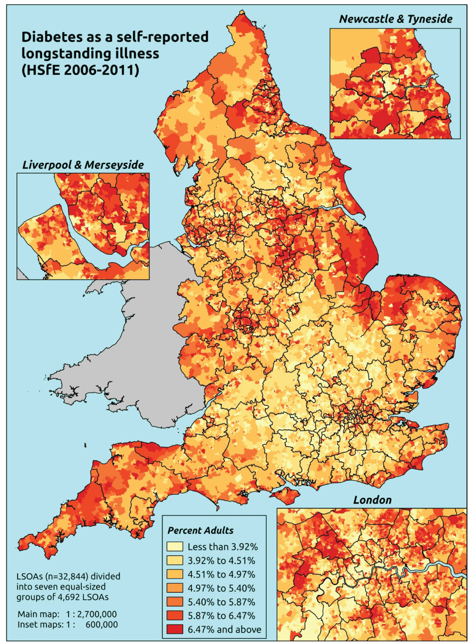
Response variable definition, provenance and prediction
These estimates are based on respondents to the HSfE reporting that diabetes is one of up to six LSIs, disabilities or infirmities, that is, one that ‘has troubled you over a period of time, or that is likely to affect you over a period of time’. There was no necessity that the respondent considered the condition to be a limiting illness.
The HSfE at this time includes multiple household respondents of all ages. The analytical data set was drawn from the subset of respondents aged ≥ 16 years for whom data were available across all model response and predictor variables, namely whether or not they responded to the LLTI question, whether they provided responses to questions on age, sex, ethnicity, general health status, LLTI and tenure, and whether or not information is available on the IMD quintile of their LSOA of residence (n = 57,363). To avoid a potential household-level effect, a single, randomly selected adult is drawn from each household, resulting in an analytical data set of 29,905 adults aged ≥ 16 years.
| Age band (years) | Females | Age band (years) | Males | ||||
|---|---|---|---|---|---|---|---|
| Does not have condition | Has condition | % | Does not have condition | Has condition | % | ||
| 16–24 | 1361 | 4 | 0.3 | 16–24 | 1022 | 7 | 0.7 |
| 25–34 | 2655 | 24 | 0.9 | 25–34 | 1704 | 14 | 0.8 |
| 35–49 | 4471 | 85 | 1.9 | 35–49 | 3279 | 108 | 3.2 |
| 50–64 | 3767 | 204 | 5.1 | 50–64 | 3049 | 242 | 7.4 |
| 65–74 | 2045 | 231 | 10.1 | 65–74 | 1541 | 245 | 13.7 |
| 75–84 | 1591 | 186 | 10.5 | 75–84 | 942 | 147 | 13.5 |
| ≥ 85 | 624 | 41 | 6.2 | ≥ 85 | 289 | 27 | 8.5 |
| Females | 16,514 | 775 | 4.5 | Males | 11,826 | 790 | 6.3 |
| Total (males and females) | 28,340 | 1565 | 5.2 | ||||
Model parameters (see below) are applied to microsimulated LSOA-level census data to produce estimates of the number (and proportion) of people expected to report diabetes as a LSI in each age–sex cohort (and overall) in each of the 32,844 English LSOAs. As discussed in the report, bootstrapping is used to derive 95% CIs for these estimates. The bootstrapped LSOA-level prevalence rate estimates are aggregated into a number of higher geographies, namely for MSOAs, LAs, CCGs and regions (GORs), and are then used to calculate 95% CIs for these higher-level estimates. Proportionate attribution is used to restructure the estimates to align with 2001 MSOAs, as well as GP practice populations as defined by the 2011 NHS ADS.
Table 38 summarises how expected prevalence rates vary by age, sex and local deprivation (as measured by the 2010 IMD). There are 6569 LSOAs (with 9,226,227 adults) classified as being in the least deprived quintile; 6568 LSOAs (9,525,344 adults) in the second least deprived quintile; 6568 LSOAs (9,658,444 adults) in the third least deprived quintile; 6568 LSOAs (9,650,576 adults) in the fourth least deprived quintile; and 6568 LSOAs (9,535,167 adults) in the most deprived quintile. Note that, as a general rule, variations in prevalence rates reflect variations in the socioeconomic composition of populations in the different types of LSOA rather than variations in deprivation per se.
| Cohort | Least deprived quintile LSOAs | Second least deprived quintile LSOAs | Third least deprived quintile LSOAs | Fourth least deprived quintile LSOAs | Most deprived quintile LSOAs | All England |
|---|---|---|---|---|---|---|
| Female 16–24 | 0.2 (0.1 to 0.3) | 0.3(0.1 to 0.4) | 0.3(0.1 to 0.4) | 0.4(0.2 to 0.6) | 0.4(0.2 to 0.6) | 0.3(0.1 to 0.5) |
| Female 25–34 | 0.4(0.3 to 0.5) | 0.4(0.3 to 0.6) | 0.5(0.4 to 0.7) | 0.7(0.5 to 0.9) | 0.8(0.6 to 1.0) | 0.6(0.4 to 0.7) |
| Female 35–49 | 1.2(1.0 to 1.5) | 1.5(1.3 to 1.8) | 1.9(1.6 to 2.2) | 2.6(2.2 to 3.0) | 2.9(2.5 to 3.5) | 2.0(1.8 to 2.3) |
| Female 50–64 | 3.6(3.1 to 4.1) | 4.3(3.7 to 5.0) | 5.2(4.4 to 5.8) | 6.9(6.0 to 7.6) | 7.6(6.7 to 8.6) | 5.4(4.8 to 5.8) |
| Female 65–74 | 7.8(6.9 to 8.9) | 9.3(8.2 to 10.3) | 10.8(9.6 to 12.1) | 13.8(12.0 to 15.2) | 14.8(13.3 to 16.6) | 11.0(10.0 to 12.0) |
| Female ≥ 75 | 7.9(7.1 to 9.3) | 9.0(8.1 to 10.5) | 10.1(9.0 to 11.5) | 12.0(10.7 to 13.6) | 12.0(10.9 to 14.0) | 10.1(9.4 to 11.3) |
| Females | 3.4(3.0 to 4.0) | 4.0(3.5 to 4.6) | 4.5(3.9 to 5.1) | 5.1(4.5 to 5.8) | 5.1(4.5 to 5.9) | 4.4(4.0 to 4.9) |
| Male 16–24 | 0.3(0.1 to 0.5) | 0.4(0.2 to 0.5) | 0.4(0.2 to 0.6) | 0.5(0.2 to 0.8) | 0.6(0.2 to 0.9) | 0.5(0.2 to 0.7) |
| Male 25–34 | 0.6(0.4 to 0.8) | 0.7(0.5 to 0.9) | 0.8(0.6 to 1.0) | 1.0(0.7 to 1.2) | 1.0(0.8 to 1.3) | 0.8(0.6 to 1.1) |
| Male 35–49 | 1.8(1.5 to 2.1) | 2.2(1.9 to 2.6) | 2.7(2.3 to 3.1) | 3.5(3.1 to 4.1) | 3.9(3.4 to 4.6) | 2.8(2.5 to 3.3) |
| Male 50–64 | 5.5(4.6 to 6.4) | 6.6(5.7 to 7.4) | 7.8(6.7 to 8.7) | 9.8(8.6 to 10.8) | 10.2(9.0 to 11.5) | 7.9(7.1 to 8.5) |
| Male 65–74 | 11.8(10.4 to 13.4) | 13.8 (2.2 to 15.3) | 15.8(13.9 to 17.4) | 19.1 (16.9 to 20.8) | 19.6(17.4 to 22.2) | 15.7(14.4 to 17.0) |
| Male ≥ 75 | 11.9(10.5 to 13.8) | 13.5(12.2 to 15.3) | 15.0(13.7 to 16.7) | 17.3(15.7 to 19.4) | 17.0(15.4 to 19.5) | 14.7(13.6 to 16.1) |
| Males | 4.9(4.2 to 5.7) | 5.7(5.0 to 6.4) | 6.1(5.4 to 6.9) | 6.7(5.9 to 7.5) | 6.5(5.7 to 7.4) | 6.0(5.4 to 6.6) |
| All | 4.1(3.7 to 4.6) | 4.8(4.3 to 5.3) | 5.3(4.8 to 5.7) | 5.9(5.4 to 6.3) | 5.8(5.3 to 6.4) | 5.2(4.9 to 5.4) |
| Factor (reference group) | Model coefficients | 95% CI | ||
|---|---|---|---|---|
| Estimate | Standard error | 2.5% CI | 97.50% | |
| (Intercept) | –8.02423 | 0.52032 | –9.04405 | –7.00441 |
| Age (16–24 years) | ||||
| 25–34 years | 1.18027 | 0.54639 | 0.10935 | 2.25119 |
| 35–49 years | 2.23172 | 0.51060 | 1.23094 | 3.23250 |
| 50–64 years | 3.15269 | 0.50700 | 2.15898 | 4.14640 |
| 65–74 years | 3.76816 | 0.50772 | 2.77302 | 4.76329 |
| 75–84 years | 3.69604 | 0.51250 | 2.69154 | 4.70053 |
| ≥ 85 years | 3.01419 | 0.55377 | 1.92879 | 4.09959 |
| Sex (females) | ||||
| Males | 0.49556 | 0.06736 | 0.36353 | 0.62759 |
| Ethnicity (white) | ||||
| Mixed | 0.30285 | 0.34006 | –0.36368 | 0.96937 |
| Black | 0.61373 | 0.16950 | 0.28151 | 0.94596 |
| Asian | 0.97558 | 0.11934 | 0.74168 | 1.20949 |
| Other | 0.13442 | 0.47152 | –0.78977 | 1.05861 |
| General health status (very good) | ||||
| Good health | 1.31416 | 0.13971 | 1.04032 | 1.58800 |
| Fair health | 2.25396 | 0.14655 | 1.96671 | 2.54120 |
| Bad health | 2.67283 | 0.25268 | 2.17758 | 3.16809 |
| Very bad health | 2.81398 | 0.49056 | 1.85248 | 3.77547 |
| LLTI (no LTTI) | ||||
| LLTI | 2.81184 | 0.69985 | 1.44014 | 4.18354 |
| Tenure (owner–occupier) | ||||
| Social rent | 0.41757 | 0.08823 | 0.24464 | 0.59049 |
| Private rent or other tenure | –0.16827 | 0.16952 | –0.50052 | 0.16398 |
| LSOA deprivation quintile (least deprived quintile) | ||||
| Second quintile | 0.07939 | 0.09236 | –0.10164 | 0.26041 |
| Third quintile | 0.13466 | 0.09164 | –0.04495 | 0.31427 |
| Fourth quintile | 0.21888 | 0.09170 | 0.03914 | 0.39862 |
| Fifth quintile ( = most deprived quintile) | 0.04396 | 0.09770 | –0.14753 | 0.23545 |
| Interaction effects | ||||
| Male and social rent (female/owner–occupier) | –0.43283 | 0.12522 | –0.67826 | –0.18740 |
| Male and private rent (female/owner–occupier) | 0.19611 | 0.22210 | –0.23921 | 0.63143 |
| 25–34 years and LLTI (16–24 years/no LLTI) | –1.35165 | 0.71377 | –2.75064 | 0.04733 |
| 35–49 years and LLTI (16–24 years/no LLTI) | –1.67127 | 0.64981 | –2.94491 | –0.39763 |
| 50–64 years and LLTI (16–24 years/no LLTI) | –1.97253 | 0.64082 | –3.22854 | –0.71653 |
| 65–74 years and LLTI (16–24 years/no LLTI) | –1.89980 | 0.64093 | –3.15602 | –0.64358 |
| 75–84 years and LLTI (16–24 years/no LLTI) | –2.03781 | 0.64542 | –3.30283 | –0.77279 |
| ≥ 85 years and LLTI (16–24 years/no LLTI) | –1.97383 | 0.69176 | –3.32969 | –0.61798 |
| Good health and LLTI (very good health/no LLTI) | –0.44942 | 0.32863 | –1.09354 | 0.19470 |
| Fair health and LLTI (very good health/no LLTI) | –0.78714 | 0.32291 | –1.42003 | –0.15424 |
| Bad health and LLTI (very good health/no LLTI) | –0.81093 | 0.38486 | –1.56525 | –0.05661 |
| Very bad health and LLTI (very good health/no LLTI) | –0.82214 | 0.57580 | –1.95070 | 0.30642 |
FIGURE 16.
Parameter plots: self-reported diabetes as LSI.
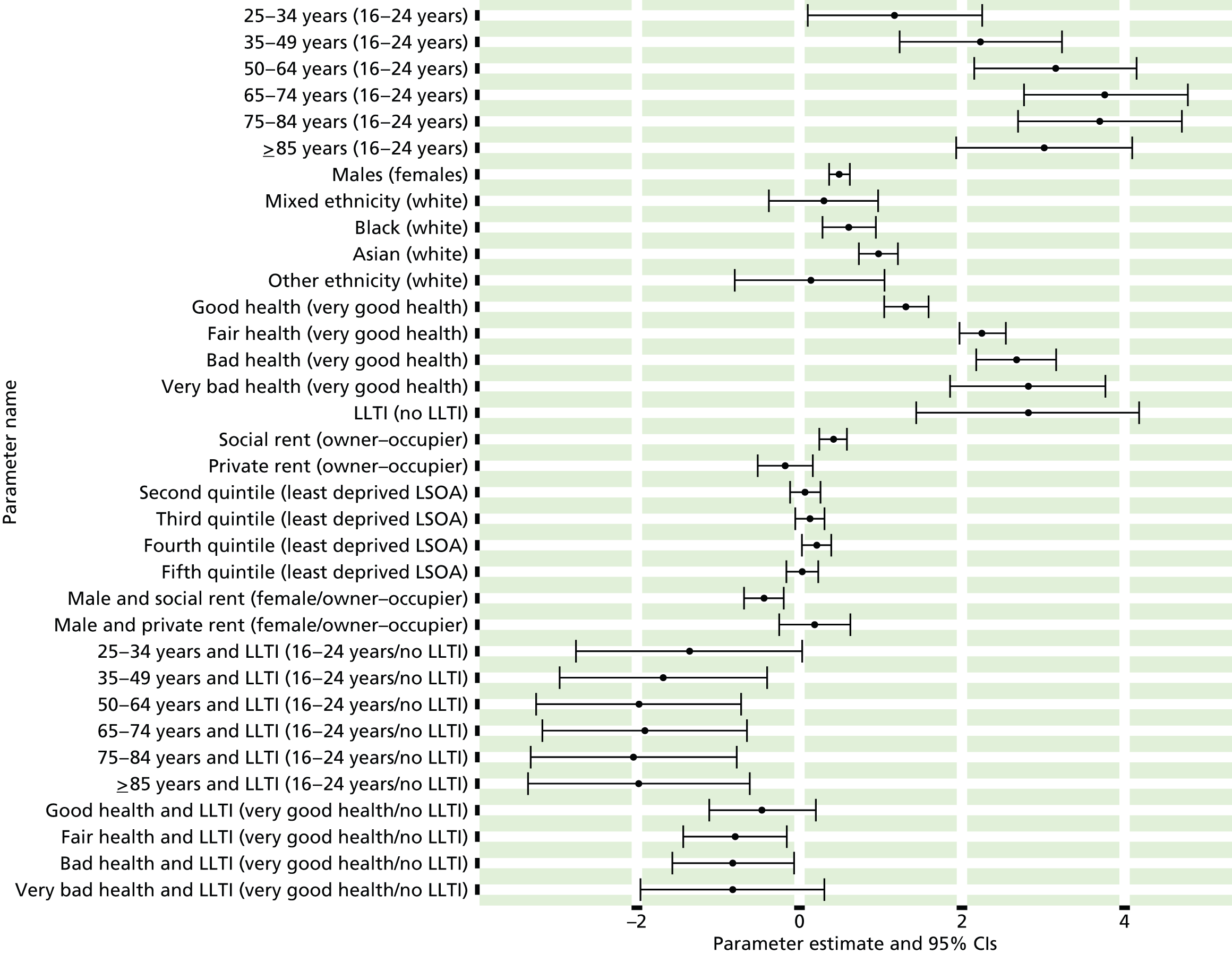
FIGURE 17.
Self-reported diabetes as LSI: individual estimates and their 95% CIs. (a) MSOAs; (b) LAs; (c) CCGs; and (d) regions (GORs).


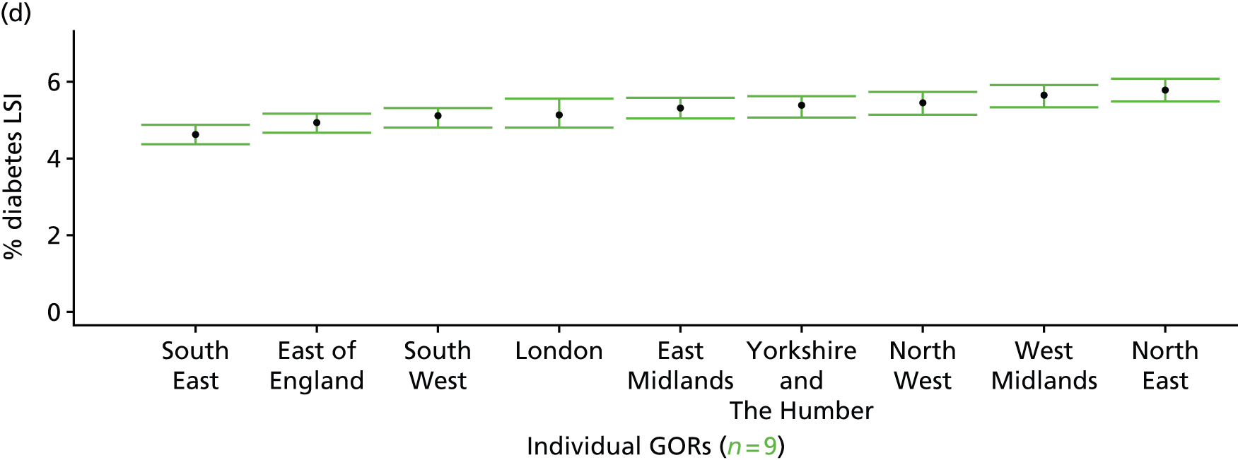
Stroke as a self-reported long-standing illness (Health Survey for England, 2006–11)
FIGURE 18.
Stroke as a self-reported LSI: LSOA-level map. Contains Ordnance Survey data © Crown copyright and database right 2012.
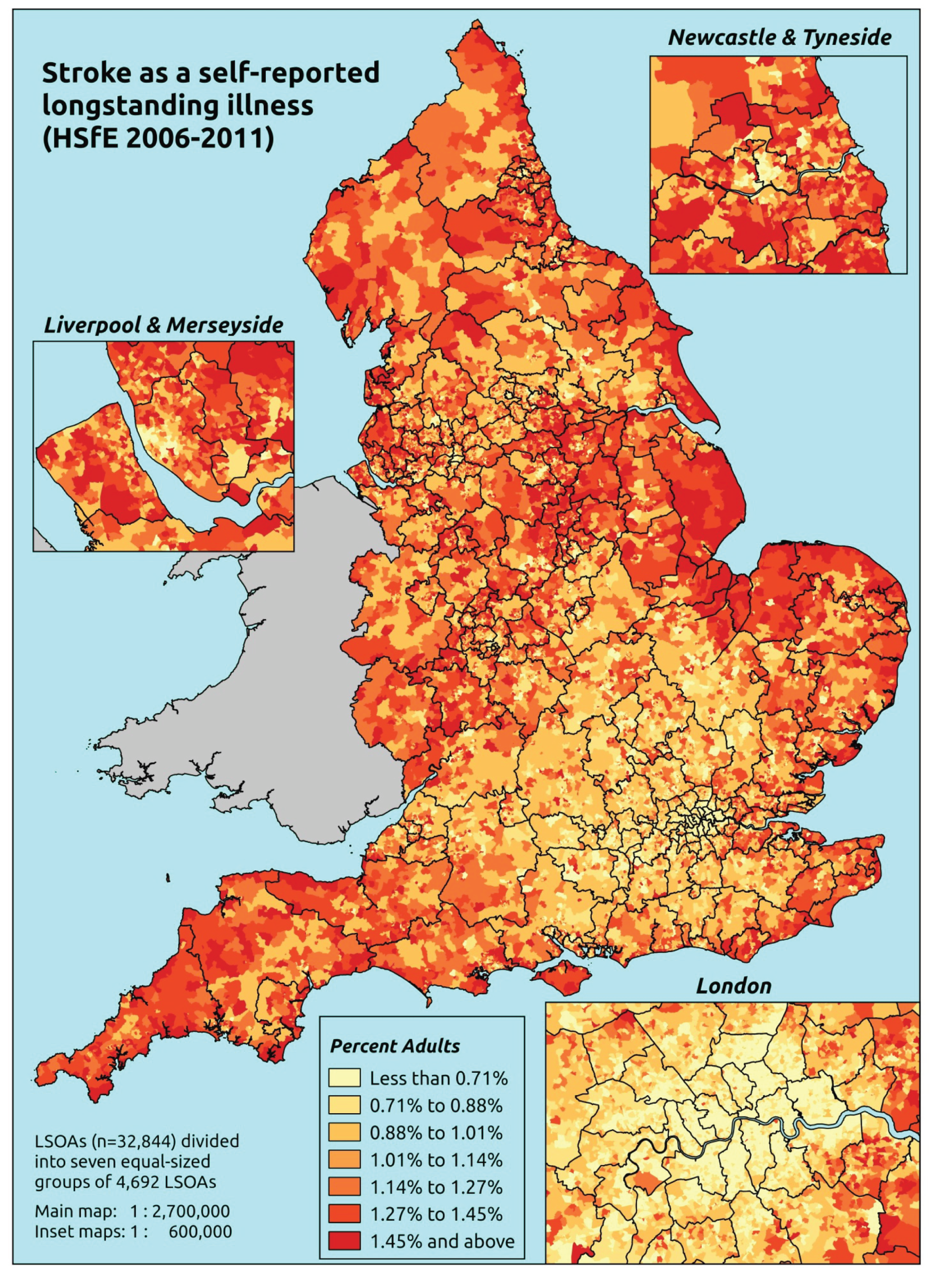
Response variable definition, provenance and prediction
These estimates are based on respondents to the HSfE reporting that a ‘stroke’ is one of up to six LSIs, disabilities or infirmities, that is, one that ‘has troubled you over a period of time, or that is likely to affect you over a period of time’. There is no necessity that the respondent considers the condition to be a limiting illness.
The HSfE at this time includes multiple household respondents of all ages. The analytical data set is drawn from the subset of respondents aged ≥ 16 years for whom data are available across all model response and predictor variables, namely whether or not they responded to the LLTI question, whether they provided responses to questions on age, sex, ethnicity, general health status, LLTI and tenure, and whether or not information is available on the IMD quintile of their LSOA of residence (n = 57,363). To avoid a potential household-level effect, a single, randomly selected adult is drawn from each household, resulting in an analytical data set of 29,905 adults aged ≥ 16 years.
| Age band (years) | Females | Age band (years) | Males | ||||
|---|---|---|---|---|---|---|---|
| Does not have condition | Has condition | % | Does not have condition | Has condition | % | ||
| 16–24 | 1365 | 0 | 0.0 | 16–24 | 1028 | 1 | 0.1 |
| 25–34 | 2677 | 2 | 0.1 | 25–34 | 1717 | 1 | 0.1 |
| 35–49 | 4547 | 9 | 0.2 | 35–49 | 3374 | 13 | 0.4 |
| 50–64 | 3938 | 33 | 0.8 | 50–64 | 3248 | 43 | 1.3 |
| 65–74 | 2250 | 26 | 1.1 | 65–74 | 1743 | 43 | 2.4 |
| 75–84 | 1730 | 47 | 2.6 | 75–84 | 1048 | 41 | 3.8 |
| ≥ 85 | 642 | 23 | 3.5 | ≥ 85 | 308 | 8 | 2.5 |
| Females | 17,149 | 140 | 0.8 | Males | 12,466 | 150 | 1.2 |
| Total (males and females) | 29,615 | 290 | 1.0 | ||||
Model parameters (see below) are applied to microsimulated LSOA-level census data to produce estimates of the number (and proportion) of people expected to report a stroke as a LSI in each age–sex cohort (and overall) in each of the 32,844 English LSOAs. As discussed in the report, bootstrapping is used to derive 95% CIs for these estimates. The bootstrapped LSOA-level prevalence rate estimates are aggregated into a number of higher geographies, namely for MSOAs, LAs, CCGs and regions (GORs), and are then used to calculate 95% CIs for these higher-level estimates. Proportionate attribution is used to restructure the estimates to align with 2001 MSOAs, as well as GP practice populations as defined by the 2011 NHS ADS.
Table 41 summarises how expected prevalence rates vary by age, sex and local deprivation (as measured by the 2010 IMD). There are 6569 LSOAs (with 9,226,227 adults) classified as being in the least deprived quintile; 6568 LSOAs (9,525,344 adults) in the second least deprived quintile; 6568 LSOAs (9,658,444 adults) in the third least deprived quintile; 6568 LSOAs (9,650,576 adults) in the fourth least deprived quintile; and 6568 LSOAs (9,535,167 adults) in the most deprived quintile. Note that, as a general rule, variations in prevalence rates reflect variations in the socioeconomic composition of populations in the different types of LSOA rather than variations in deprivation per se.
| Cohort | Least deprived quintile LSOAs | Second least deprived quintile LSOAs | Third least deprived quintile LSOAs | Fourth least deprived quintile LSOAs | Most deprived quintile LSOAs | All England |
|---|---|---|---|---|---|---|
| Female 16–24 | 0.03 (0.0 to 0.1) | 0.03 (0.0 to 0.1) | 0.03 (0.0 to 0.1) | 0.04 (0.0 to 0.1) | 0.03 (0.0 to 0.1) | 0.03 (0.0 to 0.1) |
| Female 25–34 | 0.04 (0.0 to 0.1) | 0.05 (0.0 to 0.1) | 0.05 (0.0 to 0.1) | 0.06 (0.0 to 0.1) | 0.06 (0.0 to 0.1) | 0.05 (0.0 to 0.1) |
| Female 35–49 | 0.17 (0.1 to 0.2) | 0.24 (0.1 to 0.3) | 0.25 (0.1 to 0.4) | 0.31 (0.2 to 0.5) | 0.31 (0.2 to 0.4) | 0.25 (0.1 to 0.3) |
| Female 50–64 | 0.62 (0.4 to 0.9) | 0.89 (0.6 to 1.2) | 0.96 (0.7 to 1.3) | 1.20 (0.9 to 1.6) | 1.19 (0.8 to 1.7) | 0.96 (0.7 to 1.2) |
| Female 65–74 | 1.32 (0.9 to 1.8) | 1.78 (1.2 to 2.4) | 1.83 (1.2 to 2.4) | 2.15 (1.6 to 3.0) | 2.02 (1.4 to 2.9) | 1.80 (1.3 to 2.3) |
| Female ≥ 75 | 3.18 (2.2 to 3.9) | 4.11 (3.0 to 5.0) | 3.97 (2.8 to 5.2) | 4.33 (3.2 to 5.7) | 3.61 (2.7 to 4.8) | 3.84 (3.0 to 4.6) |
| Females | 0.82 (0.6 to 1.1) | 1.09 (0.8 to 1.4) | 1.05 (0.7 to 1.4) | 1.08 (0.8 to 1.5) | 0.90 (0.6 to 1.3) | 0.99 (0.7 to 1.3) |
| Male 16–24 | 0.04 (0.0 to 0.2) | 0.04 (0.0 to 0.2) | 0.04 (0.0 to 0.2) | 0.04 (0.0 to 0.2) | 0.04 (0.0 to 0.2) | 0.04 (0.0 to 0.2) |
| Male 25–34 | 0.06 (0.0 to 0.1) | 0.08 (0.0 to 0.2) | 0.07 (0.0 to 0.2) | 0.07 (0.0 to 0.2) | 0.07 (0.0 to 0.2) | 0.07 (0.0 to 0.2) |
| Male 35–49 | 0.24 (0.1 to 0.3) | 0.33 (0.2 to 0.5) | 0.34 (0.2 to 0.5) | 0.40 (0.2 to 0.6) | 0.38 (0.2 to 0.6) | 0.34 (0.2 to 0.4) |
| Male 50–64 | 0.95 (0.7 to 1.2) | 1.32 (1.0 to 1.7) | 1.37 (1.0 to 1.8) | 1.64 (1.2 to 2.2) | 1.53 (1.1 to 2.1) | 1.35 (1.1 to 1.6) |
| Male 65–74 | 2.02 (1.3 to 2.6) | 2.74 (1.9 to 3.7) | 2.69 (1.9 to 3.5) | 3.02 (2.2 to 3.7) | 2.67 (1.8 to 3.7) | 2.61 (1.9 to 3.2) |
| Male ≥ 75 | 4.76 (3.4 to 5.6) | 5.80 (4.3 to 7.0) | 5.44 (4.0 to 6.6) | 5.71 (4.1 to 7.1) | 4.56 (3.4 to 5.9) | 5.28 (4.2 to 6.1) |
| Males | 1.12 (0.8 to 1.4) | 1.43 (1.0 to 1.9) | 1.30 (0.9 to 1.7) | 1.26 (0.9 to 1.6) | 1.01 (0.7 to 1.4) | 1.23 (0.9 to 1.5) |
| All | 0.97 (0.7 to 1.1) | 1.26 (1.0 to 1.5) | 1.17 (0.9 to 1.4) | 1.17 (0.9 to 1.4) | 0.95 (0.7 to 1.2) | 1.10 (1.0 to 1.2) |
| Factor (reference group) | Model coefficients | 95% CI | ||
|---|---|---|---|---|
| Estimate | Standard error | 2.5% CI | 97.50% | |
| (Intercept) | –9.50014 | 1.06674 | –11.5910 | –7.40932 |
| Age (16–24 years) | ||||
| 25–34 years | 0.34512 | 1.15610 | –1.92083 | 2.61108 |
| 35–49 years | 1.43970 | 1.02528 | –0.56985 | 3.44925 |
| 50–64 years | 2.26616 | 1.01147 | 0.28368 | 4.24864 |
| 65–74 years | 2.59708 | 1.01280 | 0.61198 | 4.58217 |
| 75–84 years | 2.98594 | 1.01194 | 1.00254 | 4.96934 |
| ≥ 85 years | 2.97700 | 1.02311 | 0.97172 | 4.98229 |
| Sex (females) | ||||
| Males | 0.66050 | 0.14465 | 0.37699 | 0.94401 |
| Ethnicity (white) | ||||
| Mixed | –12.8044 | 325.2716 | –650.337 | 624.7281 |
| Black | –0.00943 | 0.51826 | –1.02523 | 1.00636 |
| Asian | –0.39052 | 0.46104 | –1.29416 | 0.51312 |
| Other | –12.7936 | 434.0984 | –863.626 | 838.0392 |
| General health status (very good) | ||||
| Good health | 1.15148 | 0.38291 | 0.40098 | 1.90199 |
| Fair health | 1.96509 | 0.38182 | 1.21671 | 2.71346 |
| Bad health | 2.16646 | 0.40041 | 1.38166 | 2.95126 |
| Very bad health | 2.61358 | 0.41904 | 1.79226 | 3.43490 |
| LLTI (no LTTI) | ||||
| LLTI | 1.46941 | 0.18087 | 1.11491 | 1.82391 |
| Tenure (owner–occupier) | ||||
| Social rent | –0.04856 | 0.20663 | –0.45355 | 0.35644 |
| Private rent or other tenure | 0.48888 | 0.30666 | –0.11218 | 1.08994 |
| LSOA deprivation quintile (least deprived quintile) | ||||
| Second quintile | 0.18811 | 0.19267 | –0.18952 | 0.56575 |
| Third quintile | 0.08104 | 0.19882 | –0.30865 | 0.47072 |
| Fourth quintile | 0.09571 | 0.20057 | –0.29741 | 0.48883 |
| Fifth quintile ( = most deprived quintile) | –0.17874 | 0.22277 | –0.61537 | 0.25789 |
| Interaction effects | ||||
| Male and social rent (female/owner–occupier) | –0.35111 | 0.28882 | –0.91719 | 0.21497 |
| Male and private rent (female/owner–occupier) | –1.59649 | 0.59713 | –2.76686 | –0.42612 |
FIGURE 19.
Parameter plots: self-reported stroke as LSI.
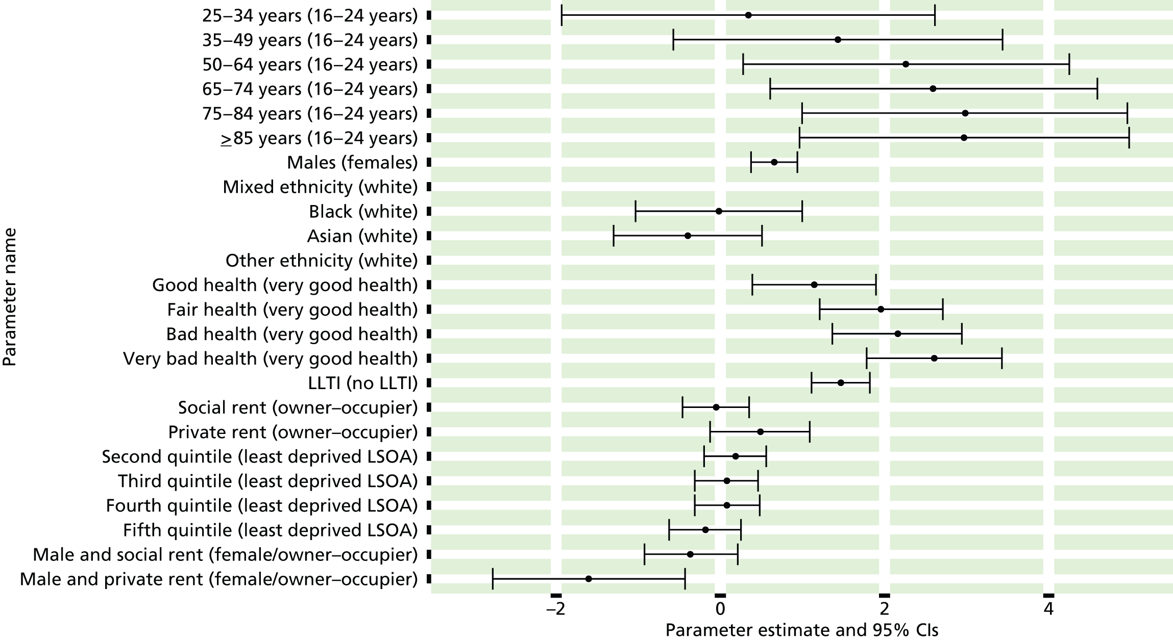
FIGURE 20.
Self-reported stroke as LSI: individual estimates and their 95% CIs: (a) MSOAs; (b) LAs; (c) CCGs; and (d) regions (GORs).


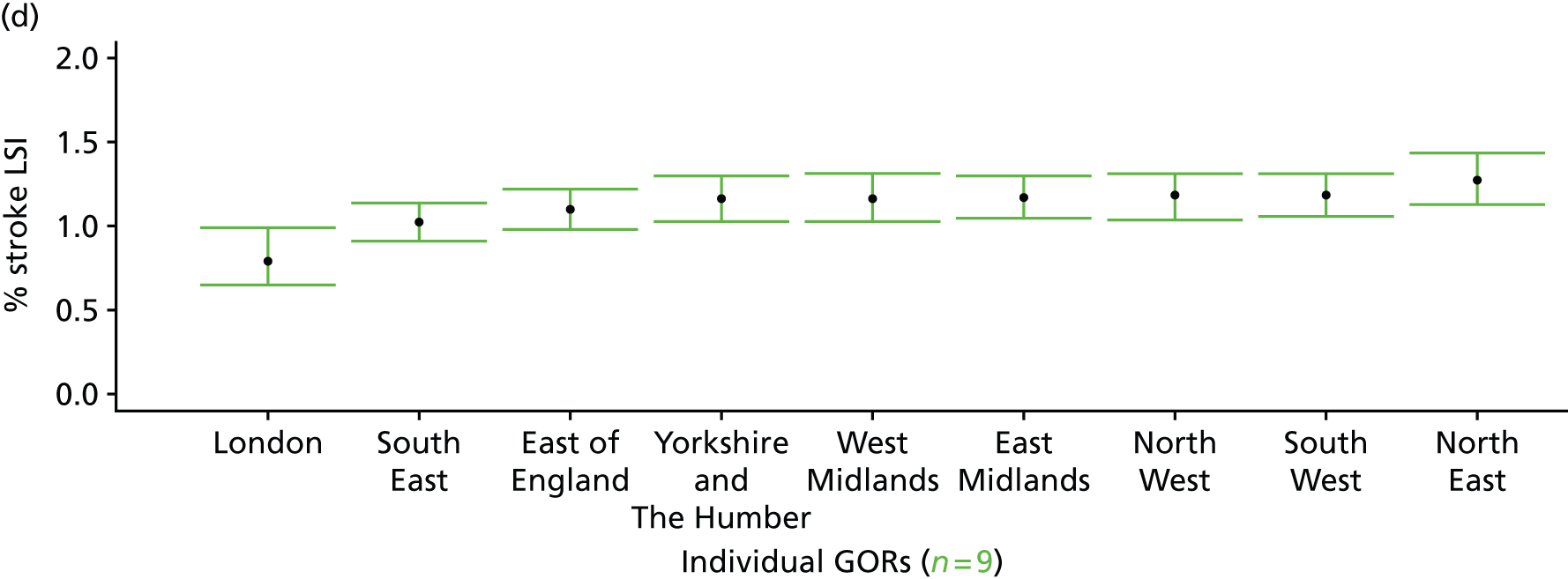
High blood pressure as a self-reported long-standing illness (Health Survey for England, 2006–11)
FIGURE 21.
High blood pressure as a self-reported LSI: LSOA-level map. Contains Ordnance Survey data © Crown copyright and database right 2012.

Response variable definition, provenance and prediction
These estimates are based on respondents to the HSfE reporting high blood pressure as one of up to six LSIs, disabilities or infirmities; that is, one that ‘has troubled you over a period of time, or that is likely to affect you over a period of time’. There is no necessity that the respondent considers the condition to be a limiting illness.
The HSfE at this time includes multiple household respondents of all ages. The analytical data set is drawn from the subset of respondents aged ≥ 16 years for whom data are available across all model response and predictor variables, namely whether or not they responded to the LLTI question, whether or not they provided responses to questions on age, sex, ethnicity, general health status, LLTI and tenure, and whether or not information is available on the IMD quintile of their LSOA of residence (n = 57,363). To avoid a potential household-level effect, a single randomly selected adult is drawn from each household, resulting in an analytical data set of 29,905 adults aged ≥ 16 years.
| Age band (years) | Females | Age band (years) | Males | ||||
|---|---|---|---|---|---|---|---|
| Does not have condition | Has condition | % | Does not have condition | Has condition | % | ||
| 16–24 | 1361 | 4 | 0.3 | 16–24 | 1028 | 1 | 0.1 |
| 25–34 | 2669 | 10 | 0.4 | 25–34 | 1709 | 9 | 0.5 |
| 35–49 | 4417 | 139 | 3.1 | 35–49 | 3279 | 108 | 3.2 |
| 50–64 | 3575 | 396 | 10.0 | 50–64 | 2907 | 384 | 11.7 |
| 65–74 | 1883 | 393 | 17.3 | 65–74 | 1493 | 293 | 16.4 |
| 75–84 | 1424 | 353 | 19.9 | 75–84 | 941 | 148 | 13.6 |
| ≥ 85 | 571 | 94 | 14.1 | ≥ 85 | 279 | 37 | 11.7 |
| Females | 15,900 | 1389 | 8.0 | Males | 11,636 | 980 | 7.8 |
| Total (males and females) | 27,536 | 2369 | 7.9 | ||||
Model parameters (see below) are applied to microsimulated LSOA-level census data to produce estimates of the number (and proportion) of people expected to report high blood pressure as a LSI in each age–sex cohort (and overall) in each of the 32,844 English LSOAs. As discussed in the report, bootstrapping is used to derive 95% CIs for these estimates. The bootstrapped LSOA-level prevalence rate estimates are aggregated into a number of higher geographies, namely for MSOAs, LAs, CCGs and regions (GORs), and are then used to calculate 95% CIs for these higher-level estimates. Proportionate attribution is used to restructure the estimates to align with 2001 MSOAs, as well as GP practice populations as defined by the 2011 NHS ADS.
Table 44 summarises how expected prevalence rates vary by age, sex and local deprivation (as measured by the 2010 IMD). There are 6569 LSOAs (with 9,226,227 adults) classified as being in the least deprived quintile; 6568 LSOAs (9,525,344 adults) in the second least deprived quintile; 6568 LSOAs (9,658,444 adults) in the third least deprived quintile; 6568 LSOAs (9,650,576 adults) in the fourth least deprived quintile; and 6568 LSOAs (9,535,167 adults) in the most deprived quintile. Note that, as a general rule, variations in prevalence rates reflect variations in the socioeconomic composition of populations in the different types of LSOA rather than variations in deprivation per se.
| Cohort | Least deprived quintile LSOAs | Second least deprived quintile LSOAs | Third least deprived quintile LSOAs | Fourth least deprived quintile LSOAs | Most deprived quintile LSOAs | All England |
|---|---|---|---|---|---|---|
| Female 16–24 | 0.2 (0.1 to 0.3) | 0.2 (0.1 to 0.3) | 0.2 (0.1 to 0.4) | 0.3 (0.1 to 0.5) | 0.3 (0.1 to 0.6) | 0.2 (0.1 to 0.5) |
| Female 25–34 | 0.2 (0.1 to 0.4) | 0.2 (0.1 to 0.4) | 0.3 (0.2 to 0.5) | 0.4 (0.2 to 0.6) | 0.4 (0.2 to 0.7) | 0.3 (0.2 to 0.5) |
| Female 35–49 | 2.3 (1.9 to 2.7) | 2.5 (2.1 to 3.0) | 3.3 (2.7 to 3.9) | 3.7 (3.0 to 4.2) | 3.7 (3.0 to 4.6) | 3.1 (2.6 to 3.5) |
| Female 50–64 | 8.1 (6.9 to 9.0) | 9.0 (7.8 to 10.0) | 11.3 (9.9 to 12.7) | 12.6 (10.7 to 13.7) | 13.2 (11.3 to 14.5) | 10.7 (9.6 to 11.4) |
| Female 65–74 | 13.6 (12.2 to 15.7) | 15.7 (14.3 to 18.4) | 18.9 (17.0 to 21.0) | 21.2 (19.0 to 23.8) | 21.9 (19.9 to 25.4) | 17.9 (16.7 to 19.6) |
| Female ≥ 75 | 14.3 (12.3 to 16.4) | 17.7 (15.5 to 19.8) | 20.3 (17.9 to 22.6) | 23.1 (20.1 to 25.1) | 23.8 (21.0 to 27.0) | 19.6 (17.9 to 21.1) |
| Females | 6.5 (5.6 to 7.4) | 7.5 (6.5 to 8.5) | 8.6 (7.5 to 9.6) | 8.6 (7.4 to 9.6) | 8.2 (7.1 to 9.5) | 7.9 (7.1 to 8.6) |
| Male 16–24 | 0.1 (0.0 to 0.2) | 0.1 (0.0 to 0.2) | 0.1 (0.0 to 0.2) | 0.1 (0.0 to 0.3) | 0.1 (0.0 to 0.4) | 0.1 (0.0 to 0.3) |
| Male 25–34 | 0.4 (0.2 to 0.8) | 0.4 (0.2 to 0.7) | 0.4 (0.2 to 0.7) | 0.5 (0.2 to 0.9) | 0.6 (0.3 to 1.1) | 0.5 (0.2 to 0.9) |
| Male 35–49 | 2.9 (2.4 to 3.5) | 2.7 (2.3 to 3.3) | 2.6 (2.1 to 3.1) | 3.3 (2.9 to 4.0) | 3.7 (3.1 to 4.5) | 3.0 (2.7 to 3.5) |
| Male 50–64 | 11.6 (10.1 to 12.8) | 11.4 (10.0 to 12.7) | 10.5 (9.0 to 11.8) | 13.2 (11.6 to 14.7) | 14.5 (12.8 to 16.3) | 12.1 (11.1 to 13.2) |
| Male 65–74 | 15.7 (13.5 to 18.0) | 15.9 (14.1 to 18.1) | 14.3 (12.5 to 16.3) | 18.3 (16.0 to 21.0) | 20.2 (17.7 to 23.3) | 16.6 (15.1 to 18.4) |
| Male ≥ 75 | 12.7 (10.0 to 14.6) | 13.9 (11.6 to 15.7) | 11.9 (9.7 to 13.8) | 15.8 (12.8 to 17.9) | 17.9 (14.4 to 20.4) | 14.1 (12.0 to 15.4) |
| Males | 7.3 (6.2 to 8.4) | 7.3 (6.3 to 8.3) | 6.1 (5.2 to 7.1) | 7.0 (6.0 to 8.1) | 7.3 (6.2 to 8.5) | 7.0 (6.2 to 7.8) |
| All | 6.9 (6.3 to 7.4) | 7.4 (6.9 to 7.8) | 7.4 (6.7 to 7.9) | 7.8 (7.3 to 8.3) | 7.8 (7.1 to 8.4) | 7.4 (7.1 to 7.7) |
| Factor (reference group) | Model coefficients | 95% CI | ||
|---|---|---|---|---|
| Estimate | Standard error | 2.5% CI | 97.50% | |
| (Intercept) | –7.35647 | 0.76286 | –8.85168 | –5.86125 |
| Age (16–24 years) | ||||
| 25–34 years | 0.68502 | 0.84678 | –0.97468 | 2.34471 |
| 35–49 years | 3.10297 | 0.76098 | 1.61145 | 4.59450 |
| 50–64 years | 4.28386 | 0.75793 | 2.79830 | 5.76941 |
| 65–74 years | 4.91661 | 0.75849 | 3.42997 | 6.40325 |
| 75–84 years | 4.98012 | 0.76021 | 3.49010 | 6.47013 |
| ≥ 85 years | 4.31465 | 0.77620 | 2.79330 | 5.83600 |
| Sex (females) | ||||
| Males | –0.85960 | 1.13391 | –3.08205 | 1.36286 |
| Ethnicity (white) | ||||
| Mixed | 0.48230 | 0.34531 | –0.19451 | 1.15911 |
| Black | 0.34554 | 0.20367 | –0.05366 | 0.74473 |
| Asian | –0.14402 | 0.18514 | –0.50690 | 0.21887 |
| Other | –1.35988 | 1.01783 | –3.35483 | 0.63508 |
| General health status (very good) | ||||
| Good health | 0.78469 | 0.09989 | 0.58890 | 0.98048 |
| Fair health | 1.28076 | 0.11407 | 1.05718 | 1.50435 |
| Bad health | 1.11981 | 0.26456 | 0.60128 | 1.63834 |
| Very bad health | 1.24532 | 0.56671 | 0.13456 | 2.35608 |
| LLTI (no LTTI) | ||||
| LLTI | 2.12768 | 0.94571 | 0.27409 | 3.98127 |
| Tenure (owner–occupier) | ||||
| Social rent | –0.15007 | 0.06306 | –0.27368 | –0.02646 |
| Private rent or other tenure | –0.18079 | 0.09711 | –0.37112 | 0.00955 |
| LSOA deprivation quintile (least deprived quintile) | ||||
| Second quintile | –0.00571 | 0.11123 | –0.22373 | 0.21231 |
| Third quintile | 0.25458 | 0.10999 | 0.03901 | 0.47016 |
| Fourth quintile | 0.21706 | 0.11561 | –0.00954 | 0.44366 |
| Fifth quintile ( = most deprived quintile) | 0.03265 | 0.12725 | –0.21676 | 0.28205 |
| Interaction effects | ||||
| Mixed and LLTI (white/no LLTI) | 0.02104 | 0.57080 | –1.09773 | 1.13981 |
| Black and LLTI (white /no LLTI) | 0.81326 | 0.29719 | 0.23077 | 1.39576 |
| Asian and LLTI (white /no LLTI) | 0.88659 | 0.25958 | 0.37781 | 1.39537 |
| Other and LLTI (white /no LLTI) | 0.31735 | 1.44729 | –2.51934 | 3.15404 |
| LLTI and second quintile (no LLTI/least deprived) | 0.33813 | 0.14886 | 0.04636 | 0.62990 |
| LLTI and third quintile (no LLTI/least deprived) | 0.19286 | 0.14970 | –0.10056 | 0.48628 |
| LLTI and fourth quintile (no LLTI/least deprived) | 0.40369 | 0.14989 | 0.10991 | 0.69746 |
| LLTI and fifth quintile (no LLTI/least deprived) | 0.60557 | 0.15638 | 0.29907 | 0.91207 |
| 25–34 years and male (16–24 years/female) | 1.35746 | 1.21547 | –1.02486 | 3.73979 |
| 35–49 years and male (16–24 years/female) | 0.88007 | 1.13122 | –1.33711 | 3.09726 |
| 50–64 years and male (16–24 years/female) | 1.02266 | 1.12632 | –1.18493 | 3.23026 |
| 65–74 years and male (16–24 years/female) | 0.78228 | 1.12704 | –1.42671 | 2.99127 |
| 75–84 years and male (16–24 years/female) | 0.41236 | 1.12904 | –1.80056 | 2.62528 |
| ≥ 85 years and male (16–24 years/female) | 0.64406 | 1.14345 | –1.59710 | 2.88522 |
| Male and second quintile (female/least deprived) | –0.14177 | 0.14296 | –0.42197 | 0.13843 |
| Male and third quintile (female/least deprived) | –0.48840 | 0.14537 | –0.77334 | –0.20347 |
| Male and fourth quintile (female/least deprived) | –0.32684 | 0.14616 | –0.61332 | –0.04035 |
| Male and fifth quintile (female/least deprived) | –0.20979 | 0.15113 | –0.50600 | 0.08642 |
| 25–34 years and LLTI (16–24 years/no LLTI) | –1.12875 | 1.03201 | –3.15149 | 0.89399 |
| 35–49 years and LLTI (16–24 years/no LLTI) | –2.02373 | 0.93026 | –3.84704 | –0.20043 |
| 50–64 years and LLTI (16–24 years/no LLTI) | –2.07281 | 0.92326 | –3.88239 | –0.26322 |
| 65–74 years and LLTI (16–24 years/no LLTI) | –2.17375 | 0.92404 | –3.98488 | –0.36263 |
| 75–84 years and LLTI (16–24 years/no LLTI) | –2.08276 | 0.92575 | –3.89722 | –0.26830 |
| ≥ 85 years and LLTI (16–24 years/no LLTI) | –1.68621 | 0.94219 | –3.53290 | 0.16048 |
| Good health and LLTI (very good health/no LLTI) | –0.14192 | 0.22110 | –0.57528 | 0.29144 |
| Fair health and LLTI (very good health/no LLTI) | –0.56433 | 0.22180 | –0.99905 | –0.12960 |
| Bad health and LLTI (very good health/no LLTI) | –0.44063 | 0.32630 | –1.08018 | 0.19892 |
| Very bad health and LLTI (very good health/no LLTI) | –0.51854 | 0.60328 | –1.70097 | 0.66388 |
| Male and good health (female/very good health) | 0.32130 | 0.15024 | 0.02682 | 0.61577 |
| Male and fair health (female/very good health) | 0.29530 | 0.15725 | –0.01292 | 0.60352 |
| Male and bad health (female/very good health) | 0.16955 | 0.20101 | –0.22442 | 0.56353 |
| Male and very bad health (female/very good health) | –0.29383 | 0.29936 | –0.88058 | 0.29292 |
FIGURE 22.
Parameter plots: self-reported high blood pressure as a LSI.
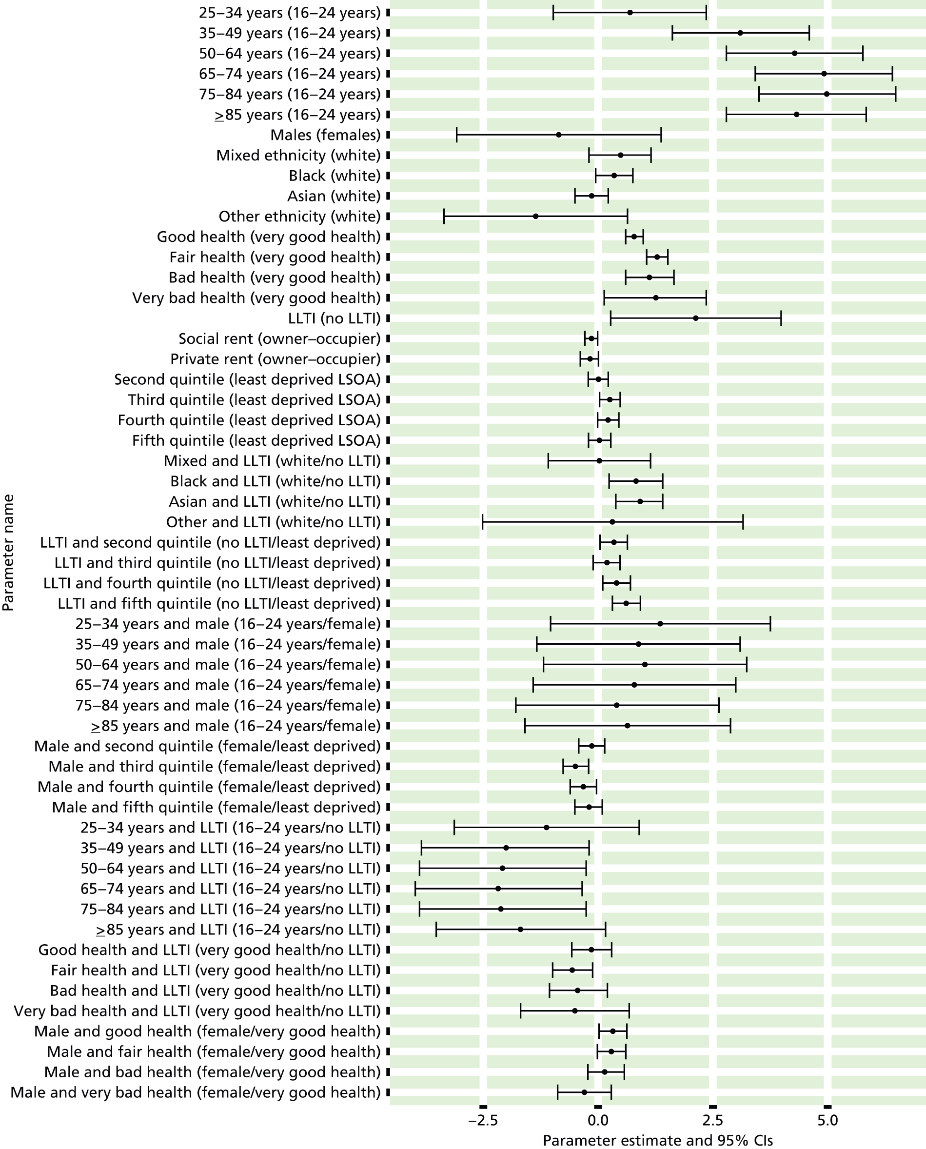
FIGURE 23.
Self-reported high blood pressure as a LSI: individual estimates and their 95% CIs: (a) MSOAs; (b) LAs; (c) CCGs; and (d) and regions (GORs). BP, blood pressure.


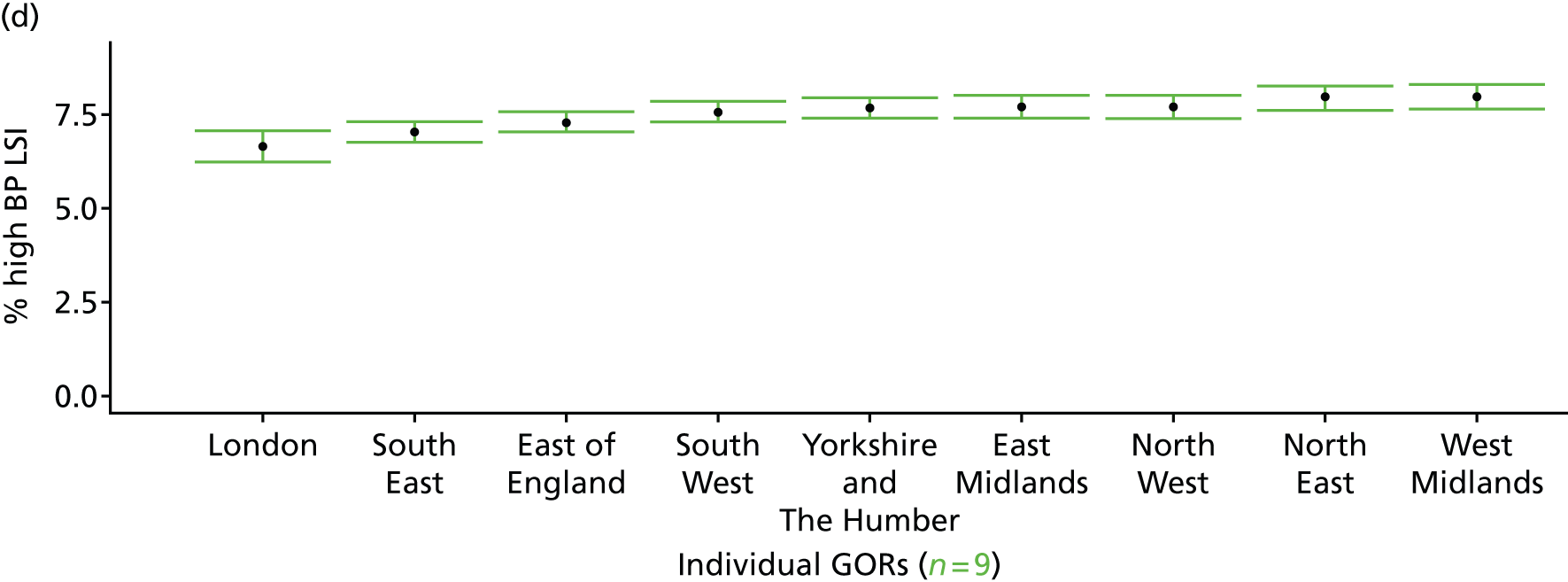
Coronary heart disease (heart attack/angina) as a self-reported long-standing illness (Health Survey for England, 2006–11)
FIGURE 24.
Coronary heart disease as a self-reported LSI: LSOA-level map. Contains Ordnance Survey data © Crown copyright and database right 2012.
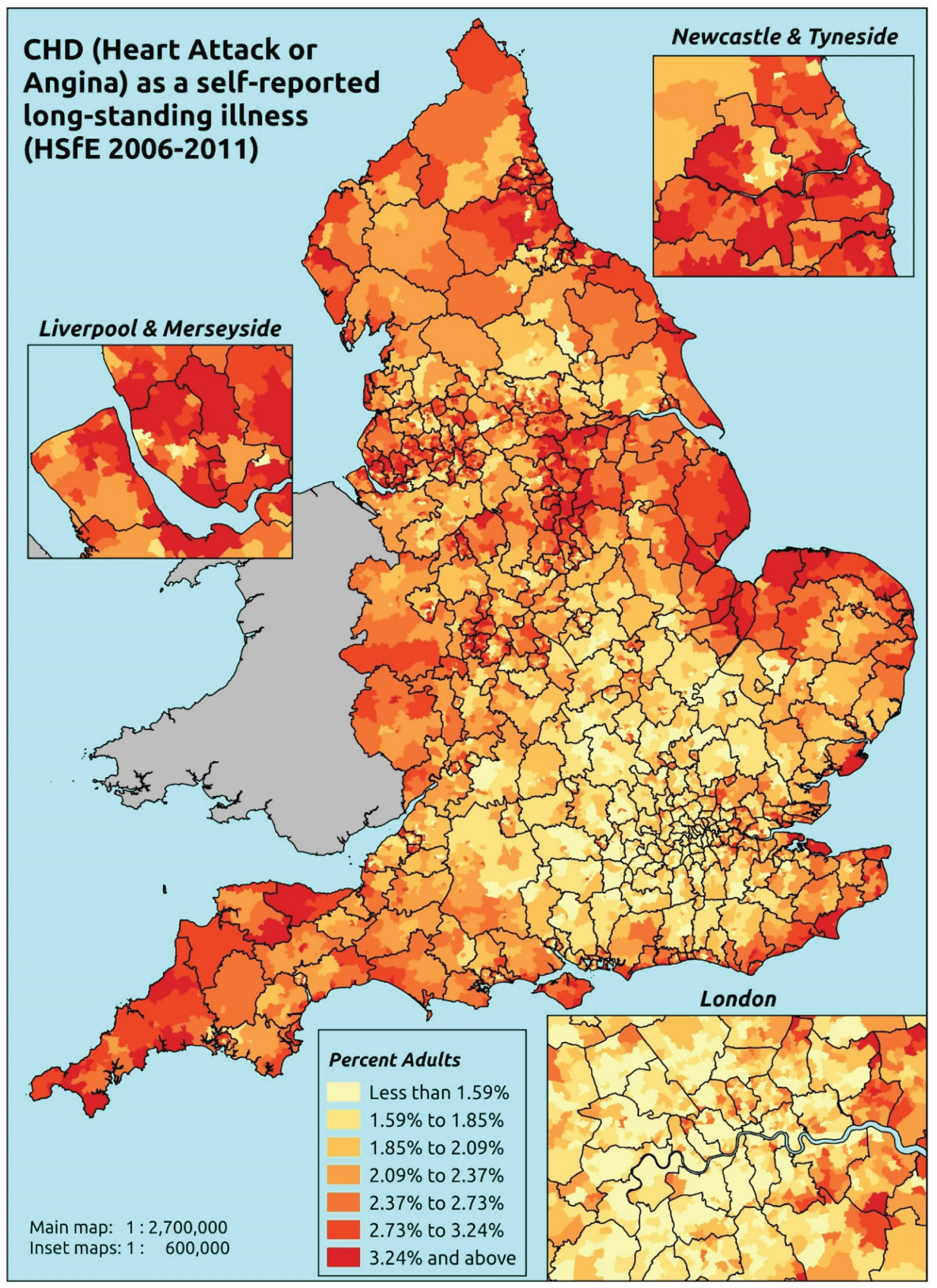
Response variable definition, provenance and prediction
These estimates are based on respondents to the HSfE reporting that a heart attack or angina (CHD) is one of up to six LSIs, disabilities or infirmities; that is, one that ‘has troubled you over a period of time, or that is likely to affect you over a period of time’. There is no necessity that the respondent considers the condition to be a limiting illness.
The HSfE at this time includes multiple household respondents of all ages. The analytical data set is drawn from the subset of respondents aged ≥ 16 years for whom data are available across all model response and predictor variables, namely whether or not they responded to the LLTI question, whether or not they provided responses to questions on age, sex, ethnicity, general health status, LLTI and tenure, and whether or not information is available on the IMD quintile of their LSOA of residence (n = 57,363). To avoid a potential household-level effect, a single randomly selected adult is drawn from each household, resulting in an analytical data set of 29,905 adults aged ≥ 16 years.
| Age band (years) | Females | Age band (years) | Males | ||||
|---|---|---|---|---|---|---|---|
| Does not have condition | Has condition | % | Does not have condition | Has condition | % | ||
| 16–24 | 1365 | 0 | 0.0 | 16–24 | 1029 | 0 | 0.0 |
| 25–34 | 2679 | 0 | 0.0 | 25–34 | 1717 | 1 | 0.1 |
| 35–49 | 4548 | 8 | 0.2 | 35–49 | 3375 | 12 | 0.4 |
| 50–64 | 3913 | 58 | 1.5 | 50–64 | 3198 | 93 | 2.8 |
| 65–74 | 2186 | 90 | 4.0 | 65–74 | 1673 | 113 | 6.3 |
| 75–84 | 1669 | 108 | 6.1 | 75–84 | 1002 | 87 | 8.0 |
| ≥ 85 | 611 | 54 | 8.1 | ≥ 85 | 300 | 16 | 5.1 |
| Females | 16,971 | 318 | 1.8 | Males | 12,294 | 322 | 2.6 |
| Total (males and females) | 29,265 | 640 | 2.1 | ||||
Model parameters (see below) are applied to microsimulated LSOA-level census data to produce estimates of the number (and proportion) of people expected to report a heart attack and/or angina (CHD) as a LSI in each age–sex cohort (and overall) in each of the 32,844 English LSOAs. As discussed in the report, bootstrapping is used to derive 95% CIs for these estimates. The bootstrapped LSOA-level prevalence rate estimates are aggregated into a number of higher geographies, namely for MSOAs, LAs, CCGs and regions (GORs), and are then used to calculate 95% CIs for these higher-level estimates. Proportionate attribution is used to restructure the estimates to align with 2001 MSOAs, as well as GP practice populations as defined by the 2011 NHS ADS.
Table 47 summarises how expected prevalence rates vary by age, sex and local deprivation (as measured by the 2010 IMD). There are 6569 LSOAs (with 9,226,227 adults) classified as being in the least deprived quintile; 6568 LSOAs (9,525,344 adults) in the second least deprived quintile; 6568 LSOAs (9,658,444 adults) in the third least deprived quintile; 6568 LSOAs (9,650,576 adults) in the fourth least deprived quintile; and 6568 LSOAs (9,535,167 adults) in the most deprived quintile. Note that, as a general rule, variations in prevalence rates reflect variations in the socioeconomic composition of populations in the different types of LSOA rather than variations in deprivation per se.
| Cohort | Least deprived quintile LSOAs | Second least deprived quintile LSOAs | Third least deprived quintile LSOAs | Fourth least deprived quintile LSOAs | Most deprived quintile LSOAs | All England |
|---|---|---|---|---|---|---|
| Female 16–24 | 0.00 (0.0 to 0.0) | 0.01 (0.0 to 0.0) | 0.00 (0.0 to 0.0) | 0.01 (0.0 to 0.0) | 0.01 (0.0 to 0.0) | 0.01 (0.0 to 0.0) |
| Female 25–34 | 0.00 (0.0 to 0.0) | 0.01 (0.0 to 0.0) | 0.01 (0.0 to 0.0) | 0.01 (0.0 to 0.0) | 0.01 (0.0 to 0.0) | 0.01 (0.0 to 0.0) |
| Female 35–49 | 0.08 (0.1 to 0.1) | 0.13 (0.1 to 0.2) | 0.14 (0.1 to 0.2) | 0.25 (0.2 to 0.4) | 0.30 (0.2 to 0.5) | 0.18 (0.1 to 0.3) |
| Female 50–64 | 0.74 (0.5 to 1.0) | 1.27 (0.9 to 1.6) | 1.23 (1.0 to 1.6) | 2.50 (2.0 to 3.0) | 2.76 (2.2 to 3.3) | 1.63 (1.4 to 1.9) |
| Female 65–74 | 2.33 (1.7 to 3.0) | 3.98 (3.1 to 5.1) | 3.73 (3.0 to 4.7) | 7.18 (6.0 to 8.4) | 7.30 (5.8 to 9.1) | 4.68 (4.1 to 5.3) |
| Female ≥ 75 | 4.17 (3.1 to 5.6) | 7.16 (5.4 to 8.9) | 6.24 (4.8 to 8.0) | 11.49 (9.6 to 13.3) | 10.18 (8.4 to 12.4) | 7.66 (6.6 to 8.7) |
| Females | 1.09 (0.8 to 1.5) | 1.87 (1.4 to 2.4) | 1.61 (1.3 to 2.1) | 2.70 (2.2 to 3.2) | 2.38 (1.9 to 3.0) | 1.94 (1.7 to 2.2) |
| Male 16–24 | 0.01 (0.0 to 0.0) | 0.01 (0.0 to 0.0) | 0.01 (0.0 to 0.0) | 0.01 (0.0 to 0.0) | 0.02 (0.0 to 0.1) | 0.01 (0.0 to 0.0) |
| Male 25–34 | 0.02 (0.0 to 0.1) | 0.01 (0.0 to 0.0) | 0.01 (0.0 to 0.0) | 0.01 (0.0 to 0.0) | 0.03 (0.0 to 0.1) | 0.02 (0.0 to 0.0) |
| Male 35–49 | 0.25 (0.2 to 0.4) | 0.15 (0.1 to 0.3) | 0.31 (0.2 to 0.5) | 0.27 (0.2 to 0.5) | 0.61 (0.4 to 1.0) | 0.32 (0.2 to 0.5) |
| Male 50–64 | 2.13 (1.6 to 2.8) | 1.47 (1.1 to 1.9) | 2.77 (2.2 to 3.5) | 2.75 (2.1 to 3.5) | 5.34 (4.3 to 6.5) | 2.81 (2.4 to 3.2) |
| Male 65–74 | 6.04 (4.4 to 7.1) | 4.49 (3.4 to 5.8) | 7.67 (6.2 to 9.2) | 7.93 (6.1 to 9.8) | 12.93 (10.7 to 15.6) | 7.47 (6.4 to 8.4) |
| Male ≥ 75 | 9.42 (6.8 to 11.4) | 7.24 (5.5 to 9.2) | 11.21 (9.0 to 14.1) | 11.54 (9.0 to 14.0) | 16.24 (13.5 to 19.8) | 10.73 (9.3 to 11.9) |
| Males | 2.48 (1.8 to 3.1) | 1.80 (1.4 to 2.3) | 2.79 (2.2 to 3.5) | 2.44 (1.9 to 3.1) | 3.63 (3.0 to 4.5) | 2.63 (2.3 to 3.0) |
| All | 1.76 (1.4 to 2.0) | 1.84 (1.5 to 2.2) | 2.18 (1.8 to 2.6) | 2.58 (2.3 to 2.9) | 2.99 (2.7 to 3.5) | 2.27 (2.1 to 2.4) |
| Factor (reference group) | Model coefficients | 95% CI | ||
|---|---|---|---|---|
| Estimate | Standard error | 2.5% CI | 97.50% | |
| (Intercept) | –11.0173 | 1.05431 | –13.0838 | –8.9509 |
| Age (25–34 years) | ||||
| 35–49 years | 2.62842 | 1.02564 | 0.61816 | 4.63868 |
| 50–64 years | 4.38383 | 1.00529 | 2.41345 | 6.35420 |
| 65–74 years | 5.23509 | 1.00484 | 3.26560 | 7.20459 |
| 75–84 years | 5.36857 | 1.00530 | 3.39819 | 7.33895 |
| ≥ 85 years | 5.38423 | 1.01058 | 3.40349 | 7.36497 |
| Sex (females) | ||||
| Males | 1.26728 | 0.26650 | 0.74494 | 1.78962 |
| Ethnicity (white) | ||||
| Other | –0.73480 | 0.26345 | –1.25116 | –0.21843 |
| General health status (very good) | ||||
| Good health | 1.24911 | 0.25479 | 0.74972 | 1.74850 |
| Fair health | 1.99527 | 0.25534 | 1.49481 | 2.49573 |
| Bad health | 2.47480 | 0.26662 | 1.95222 | 2.99738 |
| Very bad health | 2.27282 | 0.29455 | 1.69551 | 2.85013 |
| LLTI (no LTTI) | ||||
| LLTI | 0.85767 | 0.27328 | 0.32204 | 1.39330 |
| Tenure (owner–occupier) | ||||
| Social rent | 0.14358 | 0.13700 | –0.12494 | 0.41211 |
| Private rent or other tenure | –0.28401 | 0.29843 | –0.86893 | 0.30090 |
| LSOA deprivation quintile (least deprived quintile) | ||||
| Second quintile | 0.08205 | 0.34038 | –0.58510 | 0.74919 |
| Third quintile | 0.15678 | 0.32764 | –0.48540 | 0.79895 |
| Fourth quintile | 0.08322 | 0.35619 | –0.61492 | 0.78135 |
| Fifth quintile ( = most deprived quintile) | 0.74604 | 0.31754 | 0.12367 | 1.36841 |
| Interaction effects | ||||
| Male and second quintile (female/least deprived) | –0.86778 | 0.31002 | –1.47542 | –0.26013 |
| Male and third quintile (female/least deprived) | –0.20396 | 0.30107 | –0.79407 | 0.38614 |
| Male and fourth quintile (female/least deprived) | –0.83452 | 0.29767 | –1.41794 | –0.25109 |
| Male and fifth quintile (female/least deprived) | –0.25161 | 0.29766 | –0.83503 | 0.33180 |
| LLTI and second quintile (no LLTI/least deprived) | 0.48404 | 0.33510 | –0.17275 | 1.14083 |
| LLTI and third quintile (no LLTI/least deprived) | 0.20177 | 0.31117 | –0.40813 | 0.81167 |
| LLTI and fourth quintile (no LLTI/least deprived) | 0.94541 | 0.34649 | 0.26628 | 1.62453 |
| LLTI and fifth quintile (no LLTI/least deprived) | –0.00500 | 0.29750 | –0.58810 | 0.57810 |
| Male and LLTI (female/no LLTI) | –0.43820 | 0.20426 | –0.83854 | –0.03786 |
| Male and social rent (female/owner–occupier) | –0.28720 | 0.20366 | –0.68638 | 0.11198 |
| Male and private rent (female/owner–occupier) | 0.67204 | 0.37290 | –0.05885 | 1.40293 |
FIGURE 25.
Parameter plots: CHD as a self-reported LSI.
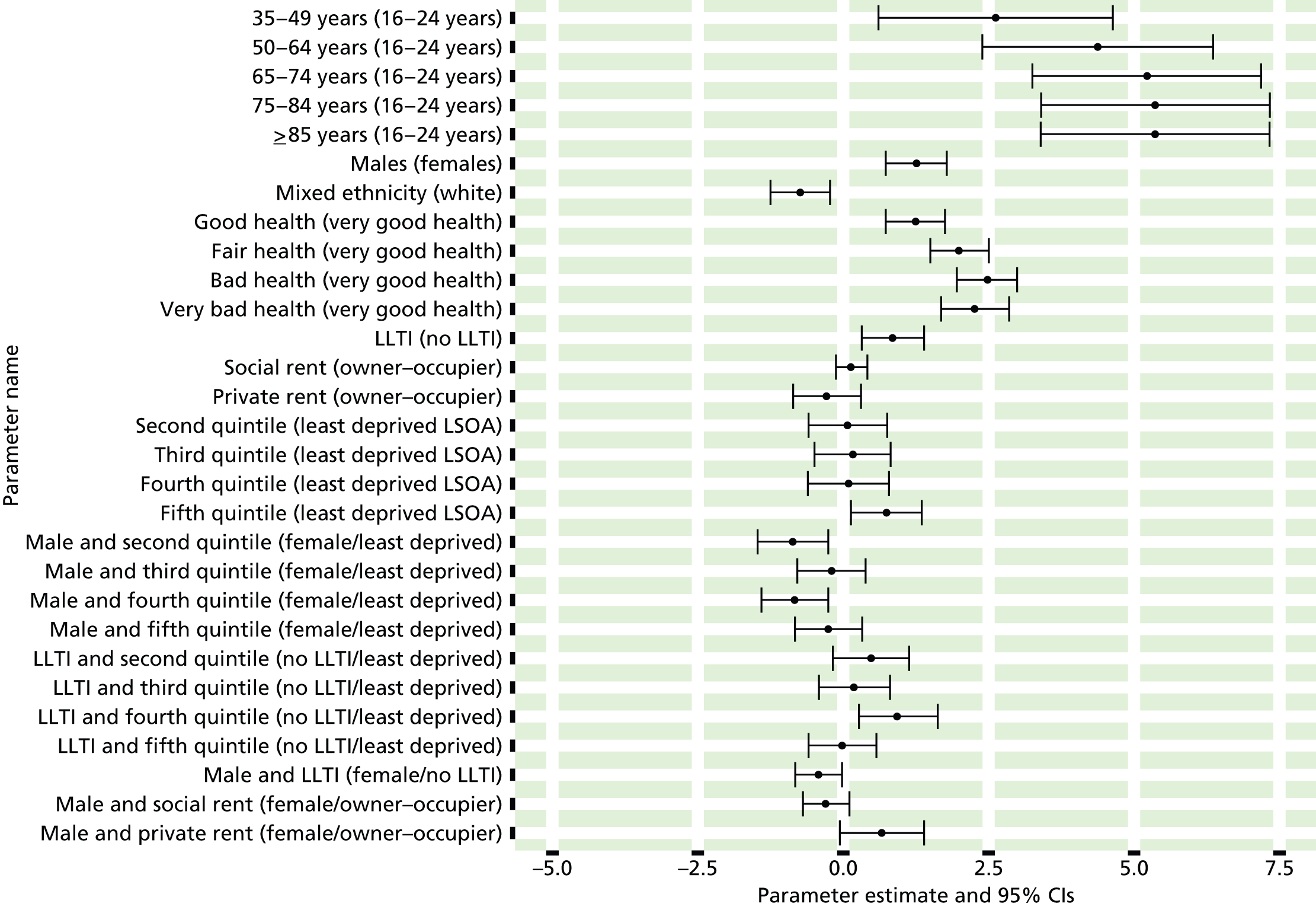
FIGURE 26.
Coronary heart disease as a self-reported LSI: individual estimates and their 95% CIs. (a) MSOAs; (b) LAs; (c), CCGs; and (d) and regions (GORs).


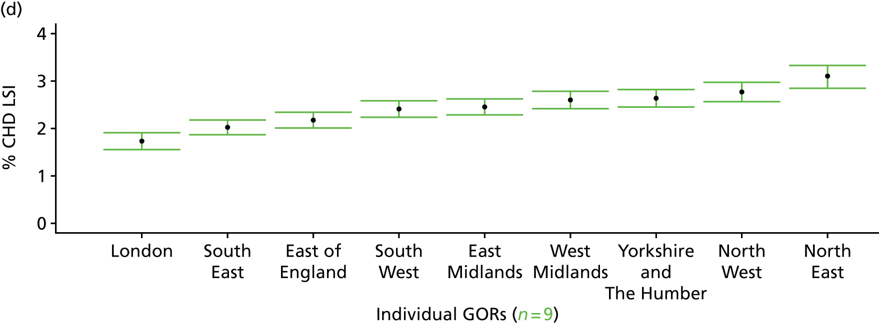
Heart failure as a self-reported long-standing illness (Health Survey for England, 2006–11)
FIGURE 27.
Heart failure as a self-reported LSI: LSOA-level map. Contains Ordnance Survey data © Crown copyright and database right 2012.

Response variable definition, provenance and prediction
These estimates are based on respondents to the HSfE reporting that a heart attack, angina or any one of a number of other heart conditions classified as ‘other heart problems’ (listed below) is one of up to six LSIs, disabilities or infirmities; that is, one that ‘has troubled you over a period of time, or that is likely to affect you over a period of time’. There is no necessity that the respondent considers the condition to be a limiting illness.
Examples given of other heart problems are aortic/mitral valve stenosis; aortic/mitral valve regurgitation; aorta replacement; atrial septal defect; cardiac asthma; cardiac diffusion; cardiac problems, heart trouble (not elsewhere specified); dizziness, giddiness, balance problems (nes); hardening of arteries in heart; heart disease, heart complaint; heart failure; heart murmur, palpitations; hole in the heart; ischaemic heart disease; pacemaker; pains in chest (nes); pericarditis; Saint Vitus dance; tachycardia, sick sinus syndrome; tired heart; valvular heart disease; weak heart because of rheumatic fever; Wolff–Parkinson–White syndrome.
The HSfE at this time includes multiple household respondents of all ages. The analytical data set is drawn from the subset of respondents aged ≥ 16 years for whom data are available across all model response and predictor variables, namely whether or not they responded to the LLTI question, whether or not they provided responses to questions on age, sex, ethnicity, general health status, LLTI and tenure, and whether or not information is available on the IMD quintile of their LSOA of residence (n = 57,363). To avoid a potential household-level effect, a single randomly selected adult is drawn from each household, resulting in an analytical data set of 29,905 adults aged ≥ 16 years.
| Age band (years) | Females | Age band (years) | Males | ||||
|---|---|---|---|---|---|---|---|
| Does not have condition | Has condition | % | Does not have condition | Has condition | % | ||
| 16–24 | 1358 | 7 | 0.5 | 16–24 | 1022 | 7 | 0.7 |
| 25–34 | 2660 | 19 | 0.7 | 25–34 | 1714 | 4 | 0.2 |
| 35–49 | 4509 | 47 | 1.0 | 35–49 | 3334 | 53 | 1.6 |
| 50–64 | 3800 | 171 | 4.3 | 50–64 | 3046 | 245 | 7.4 |
| 65–74 | 2057 | 219 | 9.6 | 65–74 | 1510 | 276 | 15.5 |
| 75–84 | 1480 | 297 | 16.7 | 75–84 | 846 | 243 | 22.3 |
| ≥ 85 | 538 | 127 | 19.1 | ≥ 85 | 258 | 58 | 18.4 |
| Females | 16,402 | 887 | 5.1 | Males | 11,730 | 886 | 7.0 |
| Total (males and females) | 28,132 | 1773 | 5.9 | ||||
Model parameters (see below) are applied to microsimulated LSOA-level census data to produce estimates of the number (and proportion) of people expected to report CHD and/or other heart problems as a LSI in each age–sex cohort (and overall) in each of the 32,844 English LSOAs. As discussed in the report, bootstrapping is used to derive 95% CIs for these estimates. The bootstrapped LSOA-level prevalence rate estimates are aggregated into a number of higher geographies, namely for MSOAs, LAs, CCGs and regions (GORs), and are then used to calculate 95% CIs for these higher-level estimates. Proportionate attribution is used to restructure the estimates to align with 2001 MSOAs, as well as GP practice populations as defined by the 2011 NHS ADS.
Table 50 summarises how expected prevalence rates vary by age, sex and local deprivation (as measured by the 2010 IMD). There are 6569 LSOAs (with 9,226,227 adults) classified as being in the least deprived quintile; 6568 LSOAs (9,525,344 adults) in the second least deprived quintile; 6568 LSOAs (9,658,444 adults) in the third least deprived quintile; 6568 LSOAs (9,650,576 adults) in the fourth least deprived quintile; and 6568 LSOAs (9,535,167 adults) in the most deprived quintile. Note that, as a general rule, variations in prevalence rates reflect variations in the socioeconomic composition of populations in the different types of LSOA rather than variations in deprivation per se.
| Cohort | Least deprived quintile LSOAs | Second least deprived quintile LSOAs | Third least deprived quintile LSOAs | Fourth least deprived quintile LSOAs | Most deprived quintile LSOAs | All England |
|---|---|---|---|---|---|---|
| Female 16–24 | 0.3 (0.1 to 0.5) | 0.3 (0.1 to 0.5) | 0.3 (0.1 to 0.6) | 0.3 (0.1 to 0.6) | 0.4 (0.2 to 0.7) | 0.4 (0.1 to 0.6) |
| Female 25–34 | 0.4 (0.3 to 0.6) | 0.4 (0.3 to 0.7) | 0.5 (0.3 to 0.7) | 0.5 (0.3 to 0.7) | 0.7 (0.4 to 1.0) | 0.5 (0.3 to 0.8) |
| Female 35–49 | 0.7 (0.5 to 0.9) | 0.8 (0.6 to 1.1) | 0.9 (0.7 to 1.2) | 1.1 (0.9 to 1.4) | 1.5 (1.1 to 1.9) | 1.0 (0.8 to 1.3) |
| Female 50–64 | 3.4 (2.8 to 3.9) | 3.8 (3.3 to 4.4) | 4.3 (3.7 to 5.0) | 5.0 (4.2 to 5.7) | 6.9 (6.0 to 7.9) | 4.6 (4.0 to 5.1) |
| Female 65–74 | 8.8 (7.5 to 10.0) | 9.6 (8.3 to 11.1) | 10.6 (9.1 to 12.0) | 11.9 (10.1 to 13.5) | 15.4 (13.1 to 17.4) | 11.0 (9.7 to 12.2) |
| Female ≥ 75 | 19.6 (17.4 to 21.7) | 20.4 (18.6 to 22.5) | 21.6 (19.3 to 23.8) | 22.5 (20.0 to 24.5) | 26.1 (23.5 to 28.3) | 21.8 (20.1 to 23.4) |
| Females | 5.0 (4.3 to 5.7) | 5.3 (4.7 to 6.1) | 5.5 (4.8 to 6.3) | 5.4 (4.6 to 6.1) | 6.1 (5.3 to 7.0) | 5.5 (4.9 to 6.1) |
| Male 16–24 | 0.5 (0.2 to 0.7) | 0.5 (0.2 to 0.7) | 0.5 (0.2 to 0.8) | 0.5 (0.2 to 0.8) | 0.6 (0.2 to 0.9) | 0.5 (0.2 to 0.8) |
| Male 25–34 | 0.2 (0.0 to 0.3) | 0.2 (0.0 to 0.4) | 0.2 (0.0 to 0.3) | 0.2 (0.0 to 0.4) | 0.2 (0.1 to 0.5) | 0.2 (0.0 to 0.4) |
| Male 35–49 | 1.1 (0.8 to 1.4) | 1.2 (1.0 to 1.6) | 1.5 (1.1 to 1.8) | 1.6 (1.3 to 2.0) | 2.2 (1.7 to 2.7) | 1.5 (1.2 to 1.9) |
| Male 50–64 | 5.8 (4.9 to 6.6) | 6.6 (5.9 to 7.5) | 7.6 (6.4 to 8.4) | 8.6 (7.3 to 9.7) | 11.4 (10.1 to 12.7) | 7.8 (7.0 to 8.6) |
| Male 65–74 | 15.4 (13.6 to 17.1) | 16.8 (15.2 to 18.9) | 18.6 (16.5 to 20.4) | 20.5 (18.4 to 22.8) | 25.0 (22.3 to 27.9) | 18.8 (17.2 to 20.6) |
| Male ≥ 75 | 25.2 (21.9 to 27.4) | 26.2 (23.1 to 28.6) | 27.6 (24.7 to 29.5) | 28.5 (25.2 to 31.2) | 32.0 (29.0 to 34.9) | 27.6 (25.2 to 29.4) |
| Males | 6.7 (5.8 to 7.5) | 7.2 (6.3 to 8.1) | 7.3 (6.3 to 8.0) | 6.9 (5.9 to 7.7) | 7.7 (6.7 to 8.7) | 7.1 (6.4 to 7.9) |
| All | 5.8 (5.3 to 6.3) | 6.2 (5.8 to 6.7) | 6.4 (5.9 to 6.8) | 6.1 (5.5 to 6.6) | 6.9 (6.4 to 7.5) | 6.3 (6.0 to 6.5) |
| Factor (reference group) | Model coefficients | 95% CI | ||
|---|---|---|---|---|
| Estimate | Standard error | 2.5% CI | 97.50% | |
| (Intercept) | –6.69103 | 0.40631 | –7.48740 | –5.89465 |
| Age (16–24 years) | ||||
| 25–34 years | 0.27096 | 0.44600 | –0.60319 | 1.14511 |
| 35–49 years | 0.47839 | 0.41008 | –0.32537 | 1.28216 |
| 50–64 years | 1.61736 | 0.39222 | 0.84860 | 2.38612 |
| 65–74 years | 2.34731 | 0.39143 | 1.58010 | 3.11453 |
| 75–84 years | 2.74956 | 0.39024 | 1.98468 | 3.51444 |
| ≥ 85 years | 2.86345 | 0.39834 | 2.08270 | 3.64420 |
| Sex (females) | ||||
| Males | 0.50602 | 0.54487 | –0.56193 | 1.57396 |
| Ethnicity (white) | ||||
| Mixed | 0.23214 | 0.37112 | –0.49526 | 0.95953 |
| Black | –1.62162 | 0.39283 | –2.39156 | –0.85168 |
| Asian | –0.37804 | 0.19388 | –0.75840 | 0.00161 |
| Other | –0.48676 | 0.61323 | –1.68870 | 0.71517 |
| General health status (very good) | ||||
| Good health | 1.14921 | 0.13485 | 0.88490 | 1.41352 |
| Fair health | 1.94149 | 0.13634 | 1.67427 | 2.20872 |
| Bad health | 2.33773 | 0.14826 | 2.04714 | 2.62831 |
| Very bad health | 2.47812 | 0.16849 | 2.14788 | 2.80835 |
| LLTI (no LTTI) | ||||
| LLTI | 0.95930 | 0.06728 | 0.82742 | 1.09118 |
| Tenure (owner–occupier) | ||||
| Social rent | 0.17090 | 0.08713 | 0.00012 | 0.34168 |
| Private rent or other tenure | –0.05095 | 0.16395 | –0.37230 | 0.27040 |
| LSOA deprivation quintile (least deprived quintile) | ||||
| Second quintile | –0.01863 | 0.08699 | –0.18913 | 0.15188 |
| Third quintile | –0.00096 | 0.08761 | –0.17268 | 0.17075 |
| Fourth quintile | –0.02961 | 0.08969 | –0.20539 | 0.14617 |
| Fifth quintile ( = most deprived quintile) | 0.07623 | 0.09328 | –0.10659 | 0.25906 |
| Interaction effects | ||||
| 25–34 years and male (16–24 years/female) | –1.52537 | 0.77174 | –3.03798 | –0.01276 |
| 35–49 years and male (16–24 years/female) | –0.00692 | 0.57718 | –1.13820 | 1.12435 |
| 50–64 years and male (16–24 years/female) | 0.12339 | 0.55153 | –0.95760 | 1.20439 |
| 65–74 years and male (16–24 years/female) | 0.20991 | 0.55135 | –0.87073 | 1.29055 |
| 75–84 years and male (16–24 years/female) | 0.07920 | 0.55137 | –1.00149 | 1.15989 |
| ≥ 85 years and male (16–24 years/female) | –0.43840 | 0.57231 | –1.56012 | 0.68332 |
| Male and social rent (female/owner–occupier) | –0.31412 | 0.12454 | –0.55822 | –0.07003 |
| Male and private rent (female/owner–occupier) | 0.26411 | 0.22268 | –0.17234 | 0.70055 |
FIGURE 28.
Parameter plots: self-reported heart failure as a LSI.
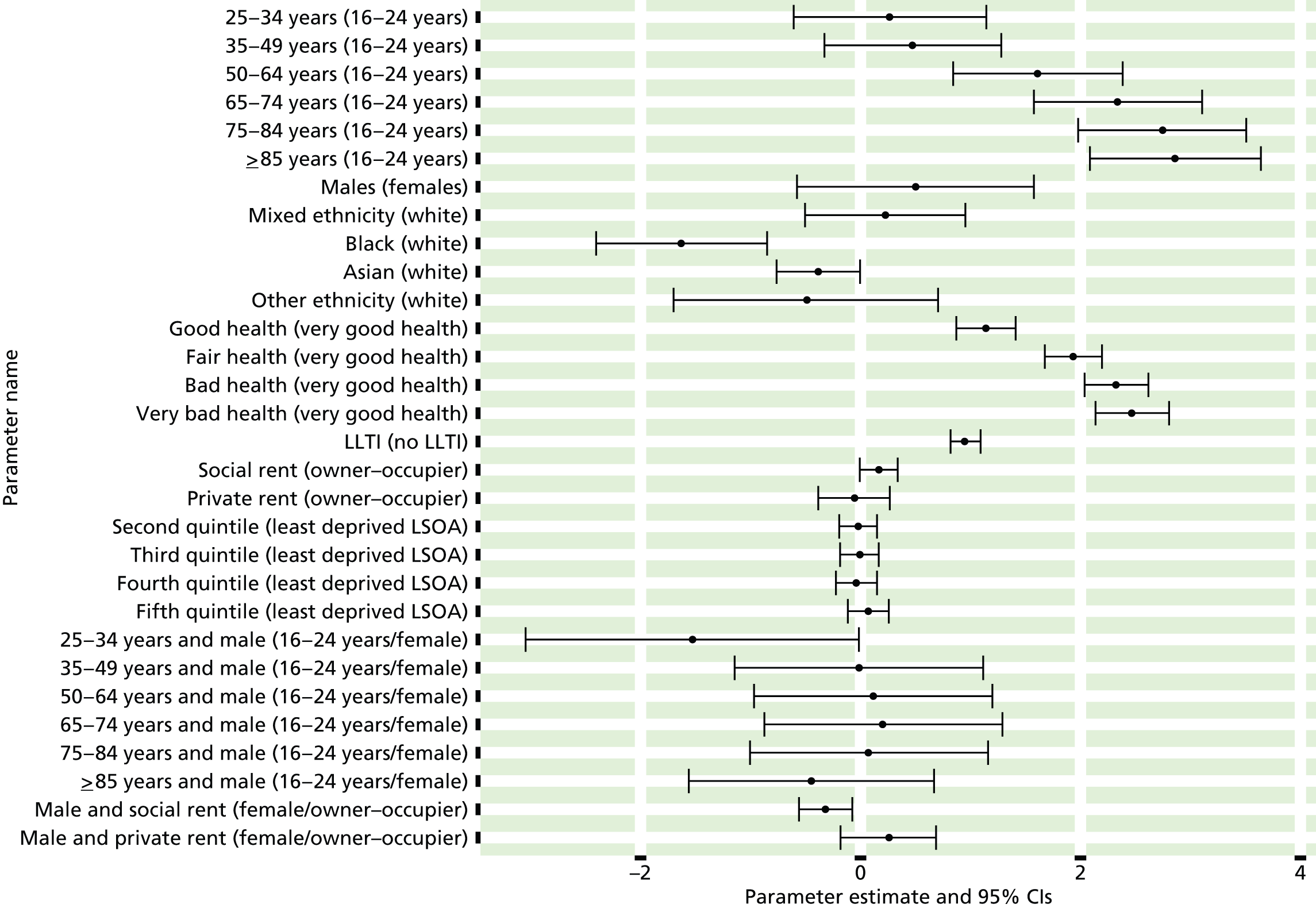
FIGURE 29.
Heart failure as a self-reported LSI: individual estimates and their 95% CIs. (a) MSOAs; (b) LAs; (c) CCGs; and (d) and regions (GORs).


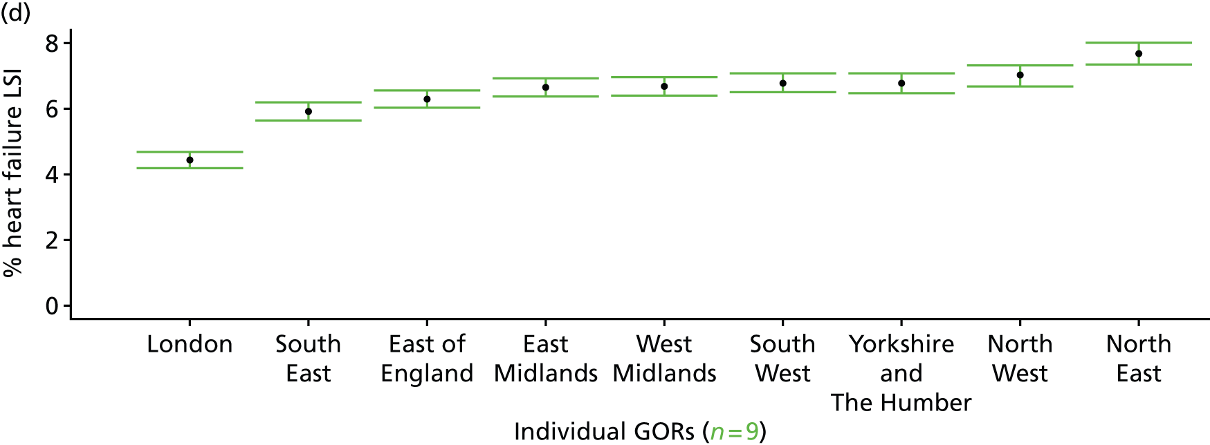
Cardiovascular disease as a self-reported long-standing illness (Health Survey for England, 2006–11)
FIGURE 30.
Cardiovascular disease as a self-reported LSI: LSOA-level map. Contains Ordnance Survey data © Crown copyright and database right 2012.
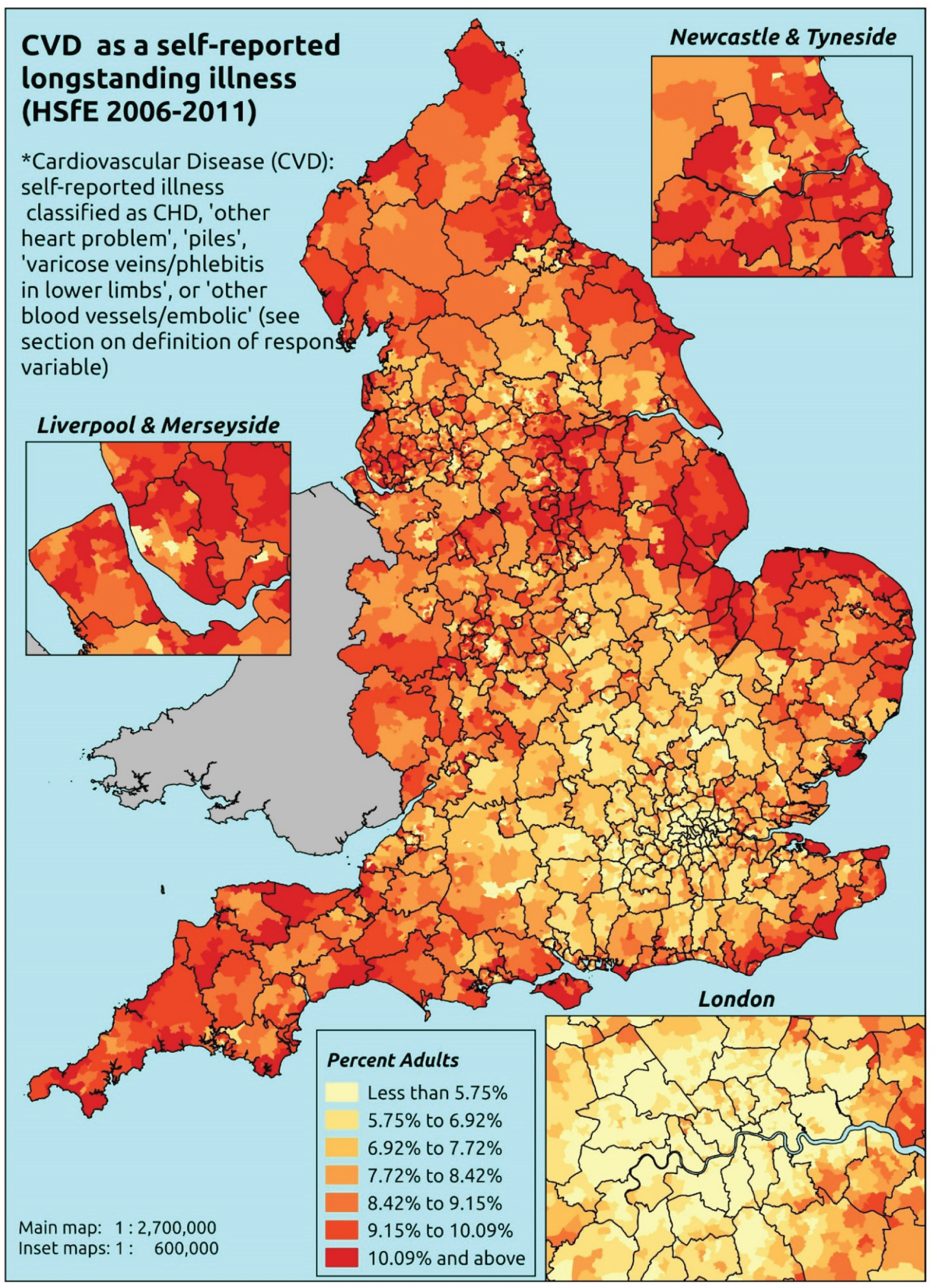
Response variable definition, provenance and prediction
These estimates are based on respondents to the HSfE reporting that a stroke, heart attack or angina (CHD), or any one of a number of other heart conditions classified as ‘other heart problem’ (see previous section), ‘piles’, ‘varicose veins/phlebitis in lower extremities’ or ‘other blood vessels/embolic’ (see below) is one of up to six LSIs, disabilities or infirmities; that is, one that ‘has troubled you over a period of time, or that is likely to affect you over a period of time’. There is no necessity that the respondent considers the condition to be a limiting illness.
For piles/haemorrhoids, the example given was varicose veins in anus.
For varicose veins/phlebitis in lower extremities, the examples given were various ulcers and varicose eczema.
For other blood vessels/embolic, the examples given were arteriosclerosis, hardening of arteries (nes); arterial thrombosis; artificial arteries (nes); blocked arteries in leg; blood clots (nes); Hand-Arm Vibration Syndrome (white finger); hypersensitive to the cold; intermittent claudication; low blood pressure/hypertension; poor circulation; pulmonary embolism; Raynaud’s disease; swollen legs and feet; telangiectasia (nes); thrombosis (nes); varicose veins in oesophagus; and Wright’s syndrome.
The HSfE at this time includes multiple household respondents of all ages. The analytical data set is drawn from the subset of respondents aged ≥ 16 years for whom data are available across all model response and predictor variables, namely whether or not they responded to the LLTI question, whether or not they provided responses to questions on age, sex, ethnicity, general health status, LLTI and tenure, and whether or not information is available on the IMD quintile of their LSOA of residence (n = 57,363). To avoid a potential household-level effect, a single randomly selected adult is drawn from each household, resulting in an analytical data set of 29,905 adults aged ≥ 16 years.
| Age band (years) | Females | Age band (years) | Males | ||||
|---|---|---|---|---|---|---|---|
| Does not have condition | Has condition | % | Does not have condition | Has condition | % | ||
| 16–24 | 1354 | 11 | 0.8 | 16–24 | 1020 | 9 | 0.9 |
| 25–34 | 2646 | 33 | 1.2 | 25–34 | 1712 | 6 | 0.3 |
| 35–49 | 4472 | 84 | 1.8 | 35–49 | 3302 | 85 | 2.5 |
| 50–64 | 3736 | 235 | 5.9 | 50–64 | 2973 | 318 | 9.7 |
| 65–74 | 2011 | 265 | 11.6 | 65–74 | 1444 | 342 | 19.1 |
| 75–84 | 1418 | 359 | 20.2 | 75–84 | 799 | 290 | 26.6 |
| ≥ 85 | 501 | 164 | 24.7 | ≥ 85 | 243 | 73 | 23.1 |
| Females | 16,138 | 1151 | 6.7 | Males | 11,493 | 1123 | 8.9 |
| Total (males and females) | 27,631 | 2274 | 7.6 | ||||
Model parameters (see below) are applied to microsimulated LSOA-level census data to produce estimates of the number (and proportion) of people expected to report CVD as a LSI in each age–sex cohort (and overall) in each of the 32,844 English LSOAs. As discussed in the report, bootstrapping is used to derive 95% CIs for these estimates. The bootstrapped LSOA-level prevalence rate estimates are aggregated into a number of higher geographies, namely for MSOAs, LAs, CCGs and regions (GORs), and are then used to calculate 95% CIs for these higher-level estimates. Proportionate attribution is used to restructure the estimates to align with 2001 MSOAs, as well as GP practice populations as defined by the 2011 NHS ADS.
Table 53 summarises how expected prevalence rates vary by age, sex and local deprivation (as measured by the 2010 IMD). There are 6569 LSOAs (with 9,226,227 adults) classified as being in the least deprived quintile; 6568 LSOAs (9,525,344 adults) in the second least deprived quintile; 6568 LSOAs (9,658,444 adults) in the third least deprived quintile; 6568 LSOAs (9,650,576 adults) in the fourth least deprived quintile; and 6568 LSOAs (9,535,167 adults) in the most deprived quintile. Note that, as a general rule, variations in prevalence rates reflect variations in the socioeconomic composition of populations in the different types of LSOA rather than variations in deprivation per se.
| Cohort | Least deprived quintile LSOAs | Second least deprived quintile LSOAs | Third least deprived quintile LSOAs | Fourth least deprived quintile LSOAs | Most deprived quintile LSOAs | All England |
|---|---|---|---|---|---|---|
| Female 16–24 | 0.5 (0.3 to 0.8) | 0.5 (0.3 to 0.8) | 0.5 (0.3 to 0.9) | 0.6 (0.3 to 0.9) | 0.7 (0.3 to 1.0) | 0.6 (0.3 to 0.9) |
| Female 25–34 | 0.7 (0.5 to 1.0) | 0.8 (0.5 to 1.1) | 0.9 (0.6 to 1.2) | 0.9 (0.6 to 1.2) | 1.1 (0.8 to 1.6) | 0.9 (0.7 to 1.2) |
| Female 35–49 | 1.3 (1.1 to 1.6) | 1.5 (1.2 to 1.9) | 1.7 (1.5 to 2.3) | 2.0 (1.7 to 2.4) | 2.6 (2.3 to 3.3) | 1.8 (1.5 to 2.3) |
| Female 50–64 | 4.5 (3.9 to 5.2) | 5.3 (4.6 to 6.0) | 6.1 (5.3 to 6.9) | 7.1 (6.2 to 7.8) | 9.3 (8.1 to 10.4) | 6.3 (5.7 to 6.9) |
| Female 65–74 | 10.5 (9.3 to 11.8) | 11.8 (10.7 to 13.2) | 13.3 (12.0 to 14.6) | 15.0 (13.2 to 16.5) | 18.2 (16.4 to 20.7) | 13.4 (12.3 to 14.8) |
| Female ≥ 75 | 24.3 (22.4 to 26.5) | 25.9 (23.8 to 28.3) | 27.5 (25.4 to 29.8) | 28.7 (26.4 to 31.0) | 31.5 (29.3 to 34.0) | 27.4 (25.9 to 29.1) |
| Females | 6.3 (5.7 to 7.1) | 7.0 (6.3 to 7.9) | 7.3 (6.6 to 8.2) | 7.2 (6.4 to 8.0) | 7.8 (7.0 to 8.9) | 7.1 (6.5 to 7.9) |
| Male 16–24 | 0.6 (0.3 to 0.9) | 0.6 (0.3 to 1.0) | 0.7 (0.3 to 1.1) | 0.7 (0.3 to 1.1) | 0.8 (0.4 to 1.3) | 0.7 (0.3 to 1.1) |
| Male 25–34 | 0.2 (0.1 to 0.4) | 0.2 (0.1 to 0.4) | 0.3 (0.1 to 0.5) | 0.3 (0.1 to 0.5) | 0.4 (0.1 to 0.6) | 0.3 (0.1 to 0.5) |
| Male 35–49 | 1.6 (1.3 to 2.0) | 1.9 (1.5 to 2.4) | 2.2 (1.8 to 2.7) | 2.6 (2.0 to 3.0) | 3.5 (2.8 to 4.3) | 2.4 (1.9 to 2.9) |
| Male 50–64 | 7.0 (6.2 to 8.0) | 8.2 (7.2 to 9.1) | 9.5 (8.4 to 10.6) | 11.0 (9.6 to 12.0) | 14.1 (12.6 to 15.7) | 9.8 (8.8 to 10.6) |
| Male 65–74 | 18.1 (16.0 to 20.3) | 20.3 (18.2 to 22.2) | 22.6 (20.5 to 24.5) | 24.9 (22.8 to 27.3) | 29.6 (27.1 to 32.2) | 22.6 (20.6 to 24.6) |
| Male ≥ 75 | 28.9 (26.0 to 31.6) | 30.8 (28.2 to 32.7) | 32.5 (29.7 to 34.8) | 33.8 (30.7 to 36.1) | 36.9 (33.5 to 39.5) | 32.2 (29.7 to 34.3) |
| Males | 8.0 (7.0 to 9.0) | 8.7 (7.8 to 9.6) | 8.9 (8.0 to 9.9) | 8.5 (7.6 to 9.4) | 9.4 (8.3 to 10.5) | 8.7 (7.8 to 9.6) |
| All | 7.1 (6.6 to 7.8) | 7.8 (7.3 to 8.4) | 8.1 (7.6 to 8.7) | 7.8 (7.3 to 8.4) | 8.6 (8.1 to 9.3) | 7.9 (7.6 to 8.2) |
| Factor (reference group) | Model coefficients | 95% CI | ||
|---|---|---|---|---|
| Estimate | Standard error | 2.5% CI | 97.50% | |
| (Intercept) | –6.28725 | 0.33250 | –6.93895 | –5.63556 |
| Age (16–24 years) | ||||
| 25–34 years | 0.34472 | 0.35283 | –0.34684 | 1.03627 |
| 35–49 years | 0.58097 | 0.32586 | –0.05772 | 1.21966 |
| 50–64 years | 1.44387 | 0.31489 | 0.82669 | 2.06105 |
| 65–74 years | 2.04848 | 0.31505 | 1.43099 | 2.66597 |
| 75–84 years | 2.47720 | 0.31394 | 1.86188 | 3.09253 |
| ≥ 85 years | 2.70555 | 0.32236 | 2.07373 | 3.33737 |
| Sex (females) | ||||
| Males | 0.25149 | 0.45588 | –0.64202 | 1.14501 |
| Ethnicity (white) | ||||
| Mixed | –0.46799 | 0.52813 | –1.50312 | 0.56715 |
| Black | –0.70740 | 0.31518 | –1.32516 | –0.08964 |
| Asian | –0.35227 | 0.23781 | –0.81837 | 0.11383 |
| Other | –11.9396 | 125.24500 | –257.4200 | 233.5407 |
| General health status (very good) | ||||
| Good health | 1.12975 | 0.13776 | 0.85975 | 1.39975 |
| Fair health | 2.02454 | 0.14504 | 1.74026 | 2.30883 |
| Bad health | 2.91564 | 0.23779 | 2.44957 | 3.38170 |
| Very bad health | 3.24765 | 0.43798 | 2.38922 | 4.10609 |
| LLTI [no LTTI) | ||||
| LLTI | 1.70721 | 0.22191 | 1.27226 | 2.14215 |
| Social rent | 0.00037 | 0.06224 | –0.12161 | 0.12236 |
| Private rent or other tenure | –0.00433 | 0.10033 | –0.20098 | 0.19232 |
| LSOA deprivation quintile [least deprived quintile) | ||||
| Second quintile | 0.02439 | 0.07927 | –0.13099 | 0.17976 |
| Third quintile | 0.06163 | 0.07962 | –0.09443 | 0.21770 |
| Fourth quintile | 0.05843 | 0.08119 | –0.10071 | 0.21756 |
| Fifth quintile ( = most deprived quintile) | 0.11593 | 0.08499 | –0.05065 | 0.28251 |
| Interaction effects | ||||
| 25–34 years and male (16–24 years/female) | –1.44281 | 0.63789 | –2.69308 | –0.19255 |
| 35–49 years and male (16–24 years/female) | 0.07781 | 0.48180 | –0.86652 | 1.02214 |
| 50–64 years and male (16–24 years/female) | 0.28905 | 0.46495 | –0.62224 | 1.20035 |
| 65–74 years and male (16–24 years/female) | 0.48273 | 0.46537 | –0.42939 | 1.39484 |
| 75–84 years and male (16–24 years/female) | 0.28919 | 0.46609 | –0.62435 | 1.20272 |
| ≥ 85 years and male (16–24 years/female) | –0.32647 | 0.48694 | –1.28087 | 0.62793 |
| Good health and LLTI (very good health/no LLTI) | –0.47808 | 0.24026 | –0.94900 | –0.00717 |
| Fair health and LLTI (very good health/no LLTI) | –0.70989 | 0.23806 | –1.176480 | –0.24330 |
| Bad health and LLTI (very good health/no LLTI) | –1.23146 | 0.30601 | –1.83124 | –0.63169 |
| Very bad health and LLTI (very good health/no LLTI) | –1.37649 | 0.48403 | –2.32520 | –0.42779 |
| Male and mixed (female/white) | 1.16619 | 0.70167 | –0.20909 | 2.54147 |
| Male and black (female/white) | –1.31878 | 0.67637 | –2.64446 | 0.00691 |
| Male and Asian (female/white) | –0.12072 | 0.33727 | –0.78176 | 0.54032 |
| Male and other (female/white) | 12.124980 | 125.24640 | –233.3580 | 257.6079 |
FIGURE 31.
Parameter plots: self-reported CVD as a LSI.
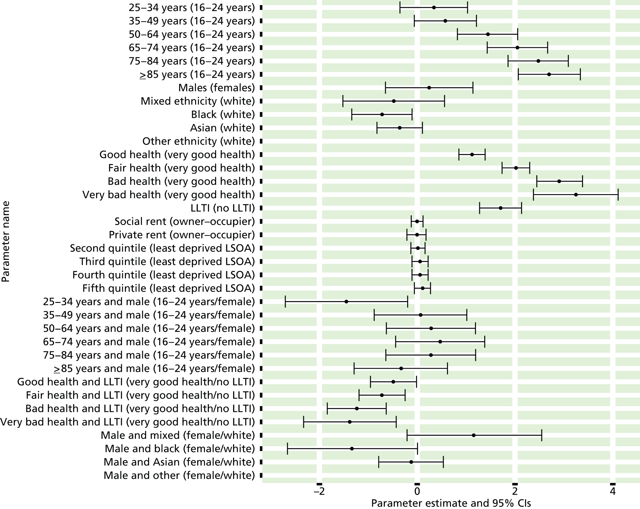
FIGURE 32.
Cardiovascular disease as a self-reported LSI: individual estimates and their 95% CIs. (a) MSOAs; (b) LAs; (c) CCGs; and (d) regions (GORs).


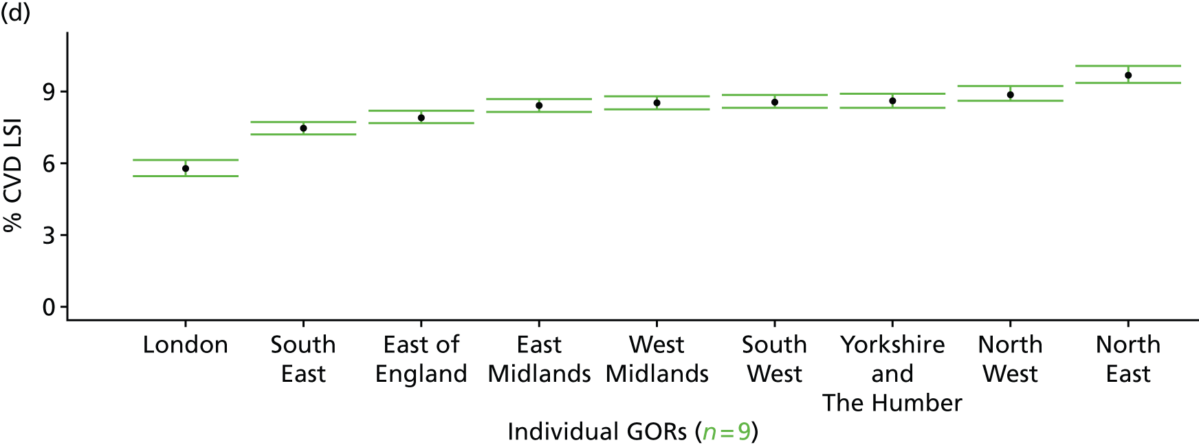
Heart/circulatory disease as a self-reported long-standing illness (Health Survey for England, 2006–11)
FIGURE 33.
Heart/circulatory disease as a self-reported LSI: LSOA-level map. Contains Ordnance Survey data © Crown copyright and database right 2012.
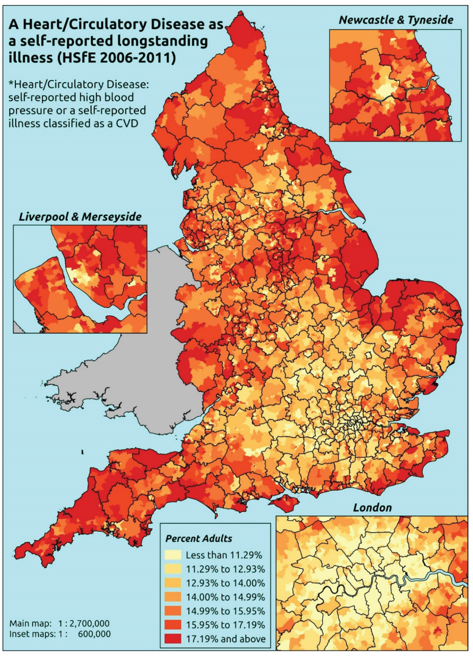
Response variable definition, provenance and prediction
These estimates are based on respondents to the HSfE reporting that CVD (see previous section) or high blood pressure (hypertension) is one of up to six LSIs, disabilities or infirmities; that is, one that ‘has troubled you over a period of time, or that is likely to affect you over a period of time’. There is no necessity that the respondent considers the condition to be a limiting illness.
The HSfE at this time includes multiple household respondents of all ages. The analytical data set is drawn from the subset of respondents aged ≥ 16 years for whom data are available across all model response and predictor variables, namely whether or not they responded to the LLTI question, whether or not they provided responses to questions on age, sex, ethnicity, general health status, LLTI and tenure, and whether or not information is available on the IMD quintile of their LSOA of residence (n = 57,363). To avoid a potential household-level effect, a single randomly selected adult is drawn from each household, resulting in an analytical data set of 29,905 adults aged ≥ 16 years.
| Age band (years) | Females | Age band (years) | Males | ||||
|---|---|---|---|---|---|---|---|
| Does not have condition | Has condition | % | Does not have condition | Has condition | % | ||
| 16–24 | 1350 | 15 | 1.1 | 16–24 | 1019 | 10 | 1.0 |
| 25–34 | 2636 | 43 | 1.6 | 25–34 | 1705 | 13 | 0.8 |
| 35–49 | 4339 | 217 | 4.8 | 35–49 | 3204 | 183 | 5.4 |
| 50–64 | 3381 | 590 | 14.9 | 50–64 | 2622 | 669 | 20.3 |
| 65–74 | 1667 | 609 | 26.8 | 65–74 | 1202 | 584 | 32.7 |
| 75–84 | 1134 | 643 | 36.2 | 75–84 | 684 | 405 | 37.2 |
| ≥ 85 | 427 | 238 | 35.8 | ≥ 85 | 215 | 101 | 32.0 |
| Females | 14,934 | 2355 | 13.6 | Males | 10,651 | 1965 | 15.6 |
| Total (males and females) | 25,585 | 4320 | 14.4 | ||||
Model parameters (see below) are applied to microsimulated LSOA-level census data to produce estimates of the number (and proportion) of people expected to report CVD or high blood pressure as a LSI in each age–sex cohort (and overall) in each of the 32,844 English LSOAs. As discussed in the report, bootstrapping is used to derive 95% CIs for these estimates. The bootstrapped LSOA-level prevalence rate estimates are aggregated into a number of higher geographies, namely for MSOAs, LAs, CCGs and regions (GORs), and are then used to calculate 95% CIs for these higher-level estimates. Proportionate attribution is used to restructure the estimates to align with 2001 MSOAs, as well as GP practice populations as defined by the 2011 NHS ADS.
Table 56 summarises how expected prevalence rates vary by age, sex and local deprivation (as measured by the 2010 IMD). There are 6569 LSOAs (with 9,226,227 adults) classified as being in the least deprived quintile; 6568 LSOAs (9,525,344 adults) in the second least deprived quintile; 6568 LSOAs (9,658,444 adults) in the third least deprived quintile; 6568 LSOAs (9,650,576 adults) in the fourth least deprived quintile; and 6568 LSOAs (9,535,167 adults) in the most deprived quintile. Note that, as a general rule, variations in prevalence rates reflect variations in the socioeconomic composition of populations in the different types of LSOA rather than variations in deprivation per se.
| Cohort | Least deprived quintile LSOAs | Second least deprived quintile LSOAs | Third least deprived quintile LSOAs | Fourth least deprived quintile LSOAs | Most deprived quintile LSOAs | All England |
|---|---|---|---|---|---|---|
| Female 16–24 | 0.7 (0.5 to 1.1) | 0.7 (0.5 to 1.1) | 0.9 (0.6 to 1.4) | 1.0 (0.7 to 1.5) | 1.0 (0.6 to 1.5) | 0.9 (0.6 to 1.4) |
| Female 25–34 | 1.0 (0.8 to 1.4) | 1.1 (0.8 to 1.5) | 1.3 (1.0 to 1.8) | 1.5 (1.1 to 2.0) | 1.6 (1.2 to 2.2) | 1.4 (1.0 to 1.8) |
| Female 35–49 | 3.6 (3.0 to 4.1) | 4.0 (3.4 to 4.4) | 4.9 (4.2 to 5.6) | 5.6 (4.9 to 6.4) | 6.1 (5.3 to 7.1) | 4.8 (4.3 to 5.4) |
| Female 50–64 | 12.0 (10.7 to 13.2) | 13.6 (12.1 to 14.9) | 16.2 (14.9 to 17.5) | 18.8 (16.4 to 20.1) | 20.3 (18.3 to 22.3) | 15.9 (14.8 to 16.8) |
| Female 65–74 | 22.2 (21.2 to 24.6) | 25.6 (23.9 to 27.8) | 29.6 (27.8 to 32.1) | 33.8 (31.2 to 35.9) | 35.8 (33.4 to 38.8) | 28.8 (27.7 to 30.6) |
| Female ≥ 75 | 34.3 (31.7 to 37.2) | 39.5 (36.2 to 42.1) | 43.1 (40.7 to 45.8) | 47.5 (44.1 to 49.7) | 47.6 (44.6 to 50.7) | 42.0 (40.2 to 43.9) |
| Females | 11.8 (10.8 to 13.1) | 13.4 (12.2 to 14.6) | 14.7 (13.5 to 15.9) | 14.9 (13.4 to 16.0) | 14.4 (13.1 to 15.8) | 13.9 (13.0 to 14.8) |
| Male 16–24 | 0.7 (0.3 to 1.1) | 0.7 (0.3 to 1.1) | 0.8 (0.3 to 1.2) | 0.8 (0.4 to 1.2) | 0.9 (0.4 to 1.5) | 0.8 (0.4 to 1.2) |
| Male 25–34 | 0.6 (0.3 to 0.9) | 0.6 (0.3 to 0.8) | 0.6 (0.3 to 0.9) | 0.6 (0.3 to 0.9) | 0.8 (0.4 to 1.2) | 0.6 (0.3 to 1.0) |
| Male 35–49 | 4.3 (3.6 to 5.0) | 4.2 (3.6 to 4.9) | 4.7 (3.9 to 5.5) | 5.1 (4.4 to 6.1) | 6.7 (5.7 to 7.7) | 5.0 (4.4 to 5.7) |
| Male 50–64 | 18.0 (16.3 to 19.6) | 18.2 (16.6 to 20.0) | 19.8 (18.0 to 21.8) | 21.6 (20.1 to 23.6) | 26.5 (24.2 to 28.5) | 20.6 (19.3 to 21.8) |
| Male 65–74 | 31.7 (29.4 to 34.1) | 32.8 (30.3 to 35.4) | 35.0 (32.3 to 37.9) | 38.1 (35.8 to 40.9) | 44.0 (40.7 to 46.7) | 35.7 (33.8 to 37.8) |
| Male ≥ 75 | 39.3 (36.0 to 42.1) | 40.8 (37.3 to 43.3) | 42.0 (38.3 to 45.1) | 44.8 (41.4 to 47.9) | 48.9 (45.0 to 52.2) | 42.6 (40.0 to 44.8) |
| Males | 14.5 (13.2 to 15.9) | 14.6 (13.3 to 16.0) | 14.5 (13.1 to 16.0) | 13.8 (12.7 to 15.2) | 15.1 (13.6 to 16.4) | 14.5 (13.5 to 15.5) |
| All | 13.1 (12.5 to 13.8) | 14.0 (13.2 to 14.6) | 14.6 (14.0 to 15.3) | 14.4 (13.7 to 15.0) | 14.7 (14.1 to 15.4) | 14.2 (13.8 to 14.5) |
| Factor (reference group) | Model coefficients | 95% CI | ||
|---|---|---|---|---|
| Estimate | Standard error | 2.5% CI | 97.50% | |
| (Intercept) | –5.56976 | 0.31175 | –6.18079 | –4.95873 |
| Age (16–24 years) | ||||
| 25–34 years | 0.30697 | 0.35463 | –0.38809 | 1.00204 |
| 35–49 years | 1.56286 | 0.30752 | 0.96012 | 2.16560 |
| 50–64 years | 2.68393 | 0.30290 | 2.09024 | 3.27762 |
| 65–74 years | 3.28657 | 0.30437 | 2.68999 | 3.88314 |
| 75–84 years | 3.55983 | 0.30673 | 2.95865 | 4.16102 |
| ≥ 85 years | 3.06663 | 0.3297 | 2.42041 | 3.71284 |
| Sex (females) | ||||
| Males | 0.00264 | 0.43397 | –0.84794 | 0.85322 |
| Ethnicity (white) | ||||
| Mixed | 0.20666 | 0.30606 | –0.39322 | 0.80654 |
| Black | 0.42884 | 0.17014 | 0.09537 | 0.76231 |
| Asian | –0.09794 | 0.15874 | –0.40907 | 0.21319 |
| Other | –1.30352 | 0.74325 | –2.76028 | 0.15325 |
| General health status (very good) | ||||
| Good health | 0.85181 | 0.08409 | 0.68698 | 1.01663 |
| Fair health | 1.35562 | 0.09191 | 1.17549 | 1.53576 |
| Bad health | 1.61205 | 0.11405 | 1.38852 | 1.83558 |
| Very bad health | 1.68238 | 0.14954 | 1.38929 | 1.97547 |
| LLTI (no LTTI) | ||||
| LLTI | 0.71164 | 0.44638 | –0.16326 | 1.58654 |
| Tenure (owner–occupier) | ||||
| Social rent | 0.00963 | 0.06558 | –0.11891 | 0.13818 |
| Private rent or other tenure | –0.08618 | 0.10405 | –0.29012 | 0.11775 |
| LSOA deprivation quintile (least deprived quintile) | ||||
| Second quintile | 0.00138 | 0.09603 | –0.18684 | 0.18960 |
| Third quintile | 0.16383 | 0.09603 | –0.02438 | 0.35204 |
| Fourth quintile | 0.14159 | 0.10094 | –0.05626 | 0.33944 |
| Fifth quintile ( = most deprived quintile) | 0.06665 | 0.10867 | –0.14635 | 0.27965 |
| Interaction effects | ||||
| 25–34 years and male (16–24 years/female) | –0.71303 | 0.52249 | –1.73712 | 0.31106 |
| 35–49 years and male (16–24 years/female) | 0.05043 | 0.42670 | –0.78590 | 0.88675 |
| 50–64 years and male (16–24 years/female) | 0.24070 | 0.41997 | –0.58244 | 1.06384 |
| 65–74 years and male (16–24 years/female) | 0.20565 | 0.42178 | –0.62104 | 1.03234 |
| 75–84 years and male (16–24 years/female) | –0.04057 | 0.42437 | –0.87233 | 0.79119 |
| ≥ 85 years and male (16–24 years/female) | –0.34762 | 0.44536 | –1.22053 | 0.52530 |
| 25–34 years and LLTI (16–24 years/no LLTI) | 0.03582 | 0.51484 | –0.97326 | 1.04490 |
| 35–49 years and LLTI (16–24 years/no LLTI) | –0.48779 | 0.44918 | –1.36819 | 0.39261 |
| 50–64 years and LLTI (16–24 years/no LLTI) | –0.54710 | 0.44132 | –1.41208 | 0.31788 |
| 65–74 years and LLTI (16–24 years/no LLTI) | –0.41937 | 0.44263 | –1.28692 | 0.44819 |
| 75–84 years and LLTI (16–24 years/no LLTI) | –0.40286 | 0.44439 | –1.27385 | 0.46814 |
| ≥ 85 years and LLTI (16–24 years/no LLTI) | 0.25405 | 0.46449 | –0.65636 | 1.16445 |
| Male and LLTI (female/no LLTI) | 0.18611 | 0.09001 | 0.00968 | 0.36253 |
| Male and social rent (female/owner–occupier) | –0.23067 | 0.10302 | –0.43259 | –0.02876 |
| Male and private rent (female/owner–occupier) | –0.14230 | 0.15568 | –0.44743 | 0.16282 |
| LLTI and second quintile (no LLTI/least deprived) | 0.22568 | 0.11842 | –0.00643 | 0.45779 |
| LLTI and third quintile (no LLTI/least deprived) | 0.16628 | 0.11826 | –0.06550 | 0.39806 |
| LLTI and fourth quintile (no LLTI/least deprived) | 0.32977 | 0.12052 | 0.09354 | 0.56599 |
| LLTI and fifth quintile (no LLTI/least deprived) | 0.30265 | 0.12325 | 0.06108 | 0.54421 |
| Male and good health (female/very good health) | 0.25148 | 0.12873 | –0.00083 | 0.50380 |
| Male and fair health (female/very good health) | 0.40373 | 0.13921 | 0.13088 | 0.67658 |
| Male and bad health (female/very good health) | 0.30832 | 0.17381 | –0.03235 | 0.64898 |
| Male and very bad health (female/very good health) | 0.19531 | 0.22776 | –0.25109 | 0.64171 |
| Male and mixed (female/white) | 0.18608 | 0.49165 | –0.77755 | 1.14970 |
| Male and black (female/white) | –0.78591 | 0.30367 | –1.38110 | –0.19072 |
| Male and Asian (female/white) | 0.10766 | 0.22648 | –0.33625 | 0.55157 |
| Male and other (female/white) | 0.92182 | 0.93191 | –0.90473 | 2.74837 |
| Male and second quintile (female/least deprived) | –0.15984 | 0.11780 | –0.39074 | 0.07105 |
| Male and third quintile (female/least deprived) | –0.26252 | 0.11853 | –0.49485 | –0.03019 |
| Male and fourth quintile (female/least deprived) | –0.31174 | 0.12248 | –0.55180 | –0.07168 |
| Male and fifth quintile (female/least deprived) | –0.10714 | 0.13086 | –0.36363 | 0.14935 |
FIGURE 34.
Parameter plots: heart/circulatory disease as a self-reported LSI.
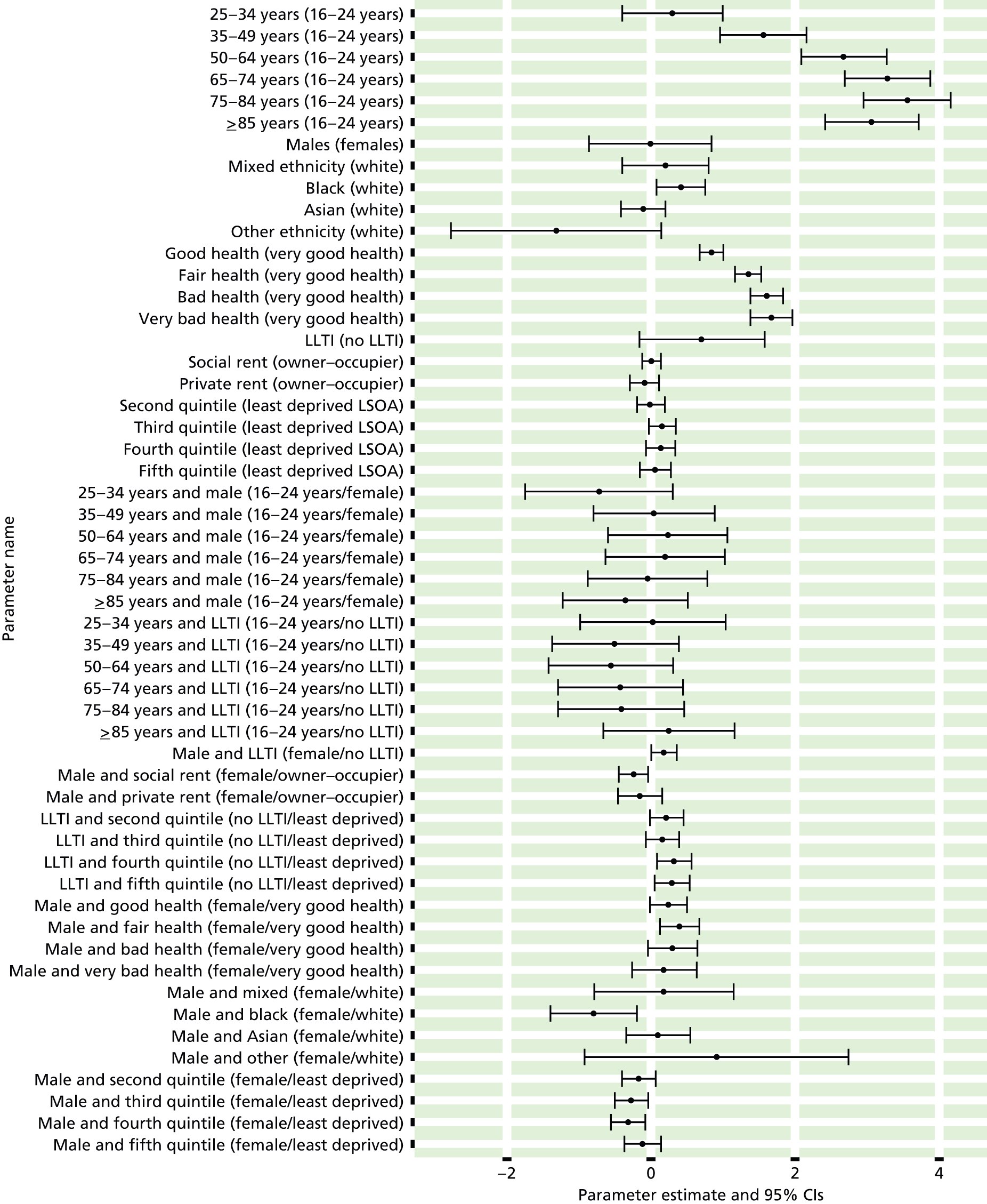
FIGURE 35.
Heart/circulatory disease as a self-reported LSI: individual estimates and their 95% CIs. (a) MSOAs; (b) LAs; (c) CCGs; and (d) regions (GORs).


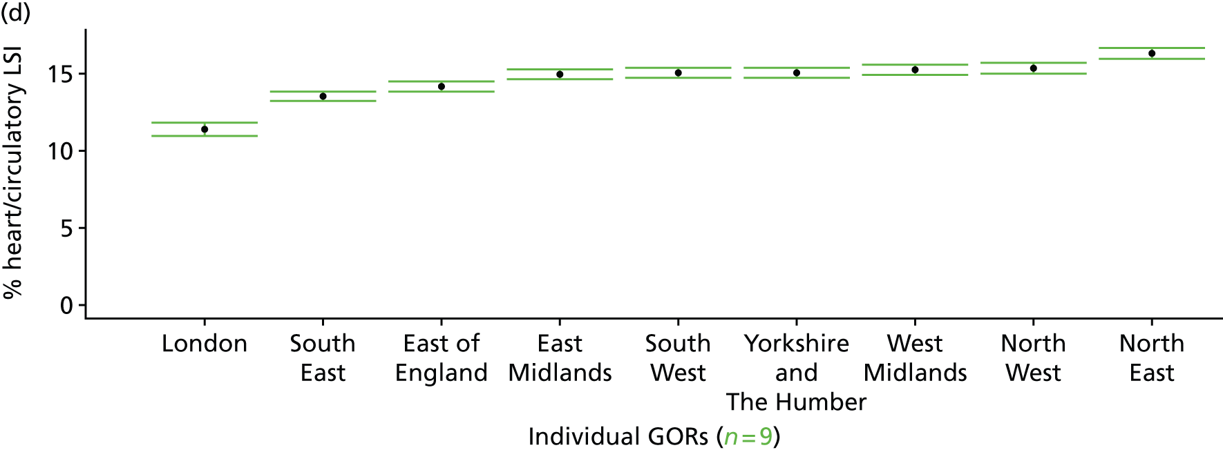
Cardiovascular disease or diabetes as a self-reported long-standing illness (Health Survey for England, 2006–11)
FIGURE 36.
Cardiovascular disease or diabetes as a self-reported LSI: LSOA-level map. Contains Ordnance Survey data © Crown copyright and database right 2012.
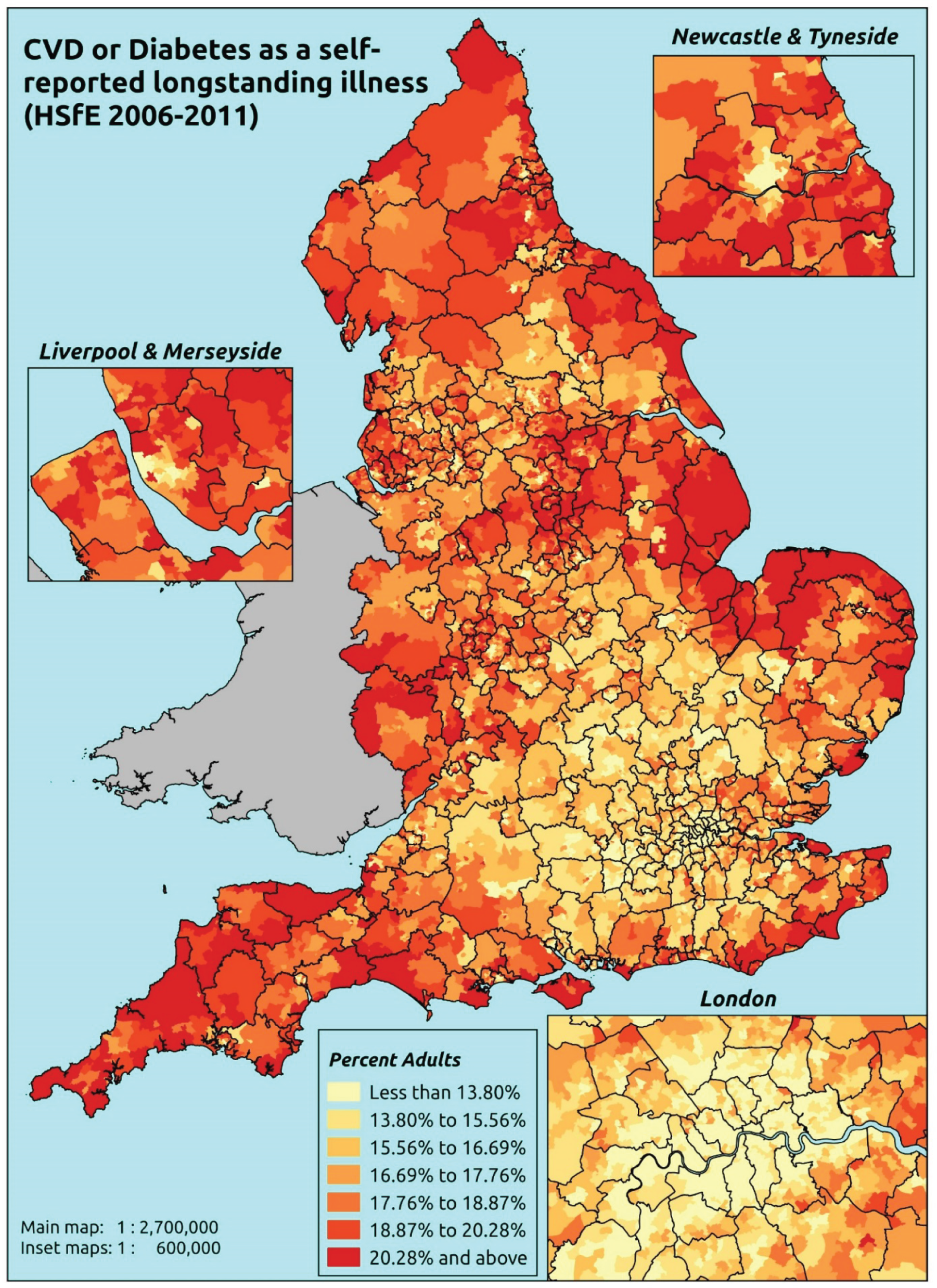
Response variable definition, provenance and prediction
These estimates are based on respondents to the HSfE reporting that CVD, high blood pressure or diabetes (see previous sections) is one of up to six LSIs, disabilities or infirmities; that is, one that ‘has troubled you over a period of time, or that is likely to affect you over a period of time’. There is no necessity that the respondent considers the condition to be a limiting illness.
The HSfE at this time includes multiple household respondents of all ages. The analytical data set is drawn from the subset of respondents aged ≥ 16 years for whom data are available across all model response and predictor variables, namely whether or not they responded to the LLTI question, whether or not they provided responses to questions on age, sex, ethnicity, general health status, LLTI and tenure, and whether or not information is available on the IMD quintile of their LSOA of residence (n = 57,363). To avoid a potential household-level effect, a single randomly selected adult is drawn from each household, resulting in an analytical data set of 29,905 adults aged ≥ 16 years.
| Age band (years) | Females | Age band (years) | Males | ||||
|---|---|---|---|---|---|---|---|
| Does not have condition | Has condition | % | Does not have condition | Has condition | % | ||
| 16–24 | 1346 | 19 | 1.4 | 16–24 | 1012 | 17 | 1.7 |
| 25–34 | 2613 | 66 | 2.5 | 25–34 | 1692 | 26 | 1.5 |
| 35–49 | 4275 | 281 | 6.2 | 35–49 | 3118 | 269 | 7.9 |
| 50–64 | 3258 | 713 | 18.0 | 50–64 | 2481 | 810 | 24.6 |
| 65–74 | 1561 | 715 | 31.4 | 65–74 | 1096 | 690 | 38.6 |
| 75–84 | 1036 | 741 | 41.7 | 75–84 | 610 | 479 | 44.0 |
| ≥ 85 | 408 | 257 | 38.6 | ≥ 85 | 201 | 115 | 36.4 |
| Females | 14,497 | 2792 | 16.1 | Males | 10,210 | 2406 | 19.1 |
| Total (males and females) | 24,707 | 5198 | 17.4 | ||||
Model parameters (see below) are applied to microsimulated LSOA-level census data to produce estimates of the number (and proportion) of people expected to report CVD, high blood pressure (hypertension) or diabetes as a LSI in each age–sex cohort (and overall) in each of the 32,844 English LSOAs. As discussed in the report, bootstrapping is used to derive 95% CIs for these estimates. The bootstrapped LSOA-level prevalence rate estimates are aggregated into a number of higher geographies, namely for MSOAs, LAs, CCGs and regions (GORs), and are then used to calculate 95% CIs for these higher-level estimates. Proportionate attribution is used to restructure the estimates to align with 2001 MSOAs, as well as GP practice populations as defined by the 2011 NHS ADS.
Table 59 summarises how expected prevalence rates vary by age, sex and local deprivation (as measured by the 2010 IMD). There are 6569 LSOAs (with 9,226,227 adults) classified as being in the least deprived quintile; 6568 LSOAs (9,525,344 adults) in the second least deprived quintile; 6568 LSOAs (9,658,444 adults) in the third least deprived quintile; 6568 LSOAs (9,650,576 adults) in the fourth least deprived quintile; and 6568 LSOAs (9,535,167 adults) in the most deprived quintile. Note that, as a general rule, variations in prevalence rates reflect variations in the socioeconomic composition of populations in the different types of LSOA rather than variations in deprivation per se.
| Cohort | Least deprived quintile LSOAs | Second least deprived quintile LSOAs | Third least deprived quintile LSOAs | Fourth least deprived quintile LSOAs | Most deprived quintile LSOAs | All England |
|---|---|---|---|---|---|---|
| Female 16–24 | 0.8 (0.5 to 1.2) | 0.9 (0.6 to 1.3) | 1.1 (0.8 to 1.6) | 1.2 (0.8 to 1.8) | 1.3 (0.9 to 1.9) | 1.1 (0.8 to 1.6) |
| Female 25–34 | 1.4 (1.1 to 1.9) | 1.7 (1.3 to 2.1) | 2.1 (1.6 to 2.6) | 2.3 (1.8 to 2.8) | 2.5 (2.0 to 3.2) | 2.1 (1.6 to 2.6) |
| Female 35–49 | 4.4 (3.9 to 5.0) | 5.0 (4.4 to 5.7) | 6.4 (5.7 to 7.2) | 7.3 (6.3 to 8.2) | 8.2 (7.3 to 9.3) | 6.2 (5.6 to 6.9) |
| Female 50–64 | 14.3 (12.9 to 15.5) | 16.4 (14.7 to 17.5) | 19.9 (18.1 to 21.1) | 22.6 (20.7 to 23.9) | 24.8 (22.6 to 26.7) | 19.3 (18.0 to 20.1) |
| Female 65–74 | 26.2 (24.4 to 28.7) | 30.2 (28.1 to 32.5) | 35.1 (33.2 to 37.3) | 39.2 (36.5 to 41.7) | 42.0 (39.9 to 45.3) | 33.9 (32.4 to 35.9) |
| Female ≥ 75 | 38.6 (36.1 to 41.9) | 44.1 (41.4 to 46.2) | 48.9 (46.1 to 51.6) | 52.7 (49.4 to 54.9) | 53.3 (50.3 to 56.4) | 47.1 (45.1 to 49.2) |
| Females | 13.8 (12.7 to 15.2) | 15.7 (14.4 to 16.9) | 17.5 (16.2 to 18.7) | 17.5 (16.0 to 18.7) | 17.2 (15.8 to 18.7) | 16.4 (15.4 to 17.3) |
| Male 16–24 | 1.2 (0.6 to 1.6) | 1.2 (0.7 to 1.7) | 1.2 (0.7 to 1.7) | 1.4 (0.8 to 2.0) | 1.6 (0.9 to 2.2) | 1.4 (0.7 to 1.8) |
| Male 25–34 | 1.0 (0.7 to 1.5) | 1.1 (0.7 to 1.5) | 1.1 (0.7 to 1.5) | 1.3 (0.9 to 1.8) | 1.5 (1.0 to 2.1) | 1.2 (0.8 to 1.7) |
| Male 35–49 | 5.9 (5.3 to 6.7) | 6.1 (5.6 to 7.1) | 6.7 (5.9 to 7.6) | 8.0 (7.1 to 9.3) | 9.4 (8.4 to 10.9) | 7.3 (6.7 to 8.1) |
| Male 50–64 | 21.5 (19.5 to 23.1) | 22.3 (20.8 to 24.2) | 23.8 (22.0 to 25.7) | 27.6 (25.6 to 30.0) | 31.0 (28.5 to 33.0) | 25.0 (23.7 to 26.2) |
| Male 65–74 | 36.9 (34.4 to 39.6) | 38.8 (36.8 to 41.7) | 40.8 (38.1 to 43.8) | 46.1 (43.3 to 49.4) | 49.9 (46.7 to 52.4) | 41.9 (40.0 to 43.9) |
| Male ≥ 75 | 44.8 (41.0 to 47.7) | 47.3 (44.3 to 50.0) | 48.4 (44.9 to 51.2) | 53.1 (49.1 to 56.2) | 54.9 (51.2 to 57.9) | 49.2 (46.5 to 51.2) |
| Males | 17.3 (15.8 to 18.7) | 17.8 (16.6 to 19.3) | 17.5 (16.0 to 18.9) | 17.6 (16.1 to 19.2) | 18.0 (16.4 to 19.4) | 17.6 (16.6 to 18.7) |
| All | 15.5 (14.8 to 16.2) | 16.7 (15.9 to 17.4) | 17.5 (16.8 to 18.2) | 17.5 (16.7 to 18.2) | 17.6 (16.8 to 18.4) | 17.0 (16.6 to 17.4) |
| Factor (reference group) | Model coefficients | 95% CI | ||
|---|---|---|---|---|
| Estimate | Standard error | 2.5% CI | 97.50% | |
| (Intercept) | –5.56429 | 0.28974 | –6.13219 | –4.99639 |
| Age (16–24 years) | ||||
| 25–34 years | 0.70170 | 0.31675 | 0.08087 | 1.32252 |
| 35–49 years | 1.73795 | 0.28576 | 1.17786 | 2.29805 |
| 50–64 years | 2.84251 | 0.28221 | 2.28938 | 3.39563 |
| 65–74 years | 3.43491 | 0.28388 | 2.87850 | 3.99132 |
| 75–84 years | 3.70361 | 0.28633 | 3.14241 | 4.26482 |
| ≥ 85 years | 3.14721 | 0.30851 | 2.54253 | 3.75188 |
| Sex (females) | ||||
| Males | 0.09979 | 0.35902 | –0.60389 | 0.80347 |
| Ethnicity (white) | ||||
| Mixed | 0.18667 | 0.28305 | –0.36811 | 0.74144 |
| Black | 0.52386 | 0.15802 | 0.21415 | 0.83357 |
| Asian | 0.12699 | 0.13797 | –0.14344 | 0.39741 |
| Other | –0.77717 | 0.54332 | –1.84207 | 0.28773 |
| General health status (very good) | ||||
| Good health | 0.95140 | 0.08388 | 0.78699 | 1.11581 |
| Fair health | 1.65270 | 0.09611 | 1.46433 | 1.84107 |
| Bad health | 2.13320 | 0.19440 | 1.75218 | 2.51422 |
| Very bad health | 2.03352 | 0.40776 | 1.23430 | 2.83273 |
| LLTI (no LTTI) | ||||
| LLTI | 1.44728 | 0.38436 | 0.69393 | 2.20063 |
| Tenure (owner–occupier) | ||||
| Social rent | 0.08154 | 0.06047 | –0.03698 | 0.20005 |
| Private rent or other tenure | –0.15803 | 0.09804 | –0.35020 | 0.03414 |
| LSOA deprivation quintile (least deprived quintile) | ||||
| Second quintile | –0.05863 | 0.07225 | –0.20024 | 0.08298 |
| Third quintile | 0.02610 | 0.07288 | –0.11675 | 0.16894 |
| Fourth quintile | –0.00315 | 0.07713 | –0.15433 | 0.14803 |
| Fifth quintile ( = most deprived quintile) | –0.04769 | 0.08319 | –0.21075 | 0.11537 |
| Interaction effects | ||||
| 25–34 years and LLTI (16–24 years/no LLTI) | –0.47437 | 0.41009 | –1.27814 | 0.32940 |
| 35–49 years and LLTI (16–24 years/no LLTI) | –0.86080 | 0.36049 | –1.56735 | –0.15424 |
| 50–64 years and LLTI (16–24 years/no LLTI) | –0.97953 | 0.35397 | –1.67331 | –0.28576 |
| 65–74 years and LLTI (16–24 years/no LLTI) | –0.82309 | 0.35590 | –1.52065 | –0.12553 |
| 75–84 years and LLTI (16–24 years/no LLTI) | –0.81347 | 0.35822 | –1.51559 | –0.11136 |
| ≥ 85 years and LLTI (16–24 years/no LLTI) | –0.25290 | 0.38079 | –0.99924 | 0.49344 |
| 25–34 years and male (16–24 years/female) | –0.77373 | 0.41570 | –1.58850 | 0.04105 |
| 35–49 years and male (16–24 years/female) | –0.10864 | 0.35441 | –0.80329 | 0.58600 |
| 50–64 years and male (16–24 years/female) | –0.00295 | 0.34918 | –0.68734 | 0.68143 |
| 65–74 years and male (16–24 years/female) | –0.01474 | 0.35150 | –0.70368 | 0.67420 |
| 75–84 years and male (16–24 years/female) | –0.22696 | 0.35438 | –0.92155 | 0.46763 |
| ≥ 85 years and male (16–24 years/female) | –0.52167 | 0.37742 | –1.26142 | 0.21808 |
| LLTI and second quintile (no LLTI/least deprived) | 0.24953 | 0.11206 | 0.02989 | 0.46917 |
| LLTI and third quintile (no LLTI/least deprived) | 0.25093 | 0.11216 | 0.03110 | 0.47077 |
| LLTI and fourth quintile (no LLTI/least deprived) | 0.40024 | 0.11413 | 0.17654 | 0.62394 |
| LLTI and fifth quintile (no LLTI/least deprived) | 0.37492 | 0.11708 | 0.14543 | 0.60440 |
| Male and good health (female/very good health) | 0.27696 | 0.11950 | 0.04275 | 0.51118 |
| Male and fair health (female/very good health) | 0.36517 | 0.12863 | 0.11305 | 0.61728 |
| Male and bad health (female/very good health) | 0.25645 | 0.16316 | –0.06334 | 0.57624 |
| Male and very bad health (female/very good health) | 0.16845 | 0.21859 | –0.26000 | 0.59689 |
| Good health and LLTI (very good health/no LLTI) | –0.29240 | 0.15826 | –0.60259 | 0.01779 |
| Fair health and LLTI (very good health/no LLTI) | –0.48816 | 0.15896 | –0.79971 | –0.17660 |
| Bad health and LLTI (very good health/no LLTI) | –0.68203 | 0.23073 | –1.13426 | –0.22980 |
| Very bad health and LLTI (very good health/no LLTI) | –0.50814 | 0.42823 | –1.34747 | 0.33119 |
| Male and LLTI (female/no LLTI) | 0.17875 | 0.08369 | 0.01471 | 0.34278 |
| Male and mixed (female/white) | 0.13399 | 0.45430 | –0.75643 | 1.02441 |
| Male and black (female/white) | –0.62927 | 0.26753 | –1.15363 | –0.10492 |
| Male and Asian (female/white) | 0.27528 | 0.19419 | –0.10535 | 0.65590 |
| Male and other (female/white) | 0.53594 | 0.72477 | –0.88461 | 1.95650 |
| Male and social rent (female/owner–occupier) | –0.21235 | 0.09092 | –0.39056 | –0.03415 |
| Male and private rent (female/owner–occupier) | 0.01826 | 0.14256 | –0.26117 | 0.29768 |
FIGURE 37.
Parameter plots: CVD or diabetes as a self-reported LSI.
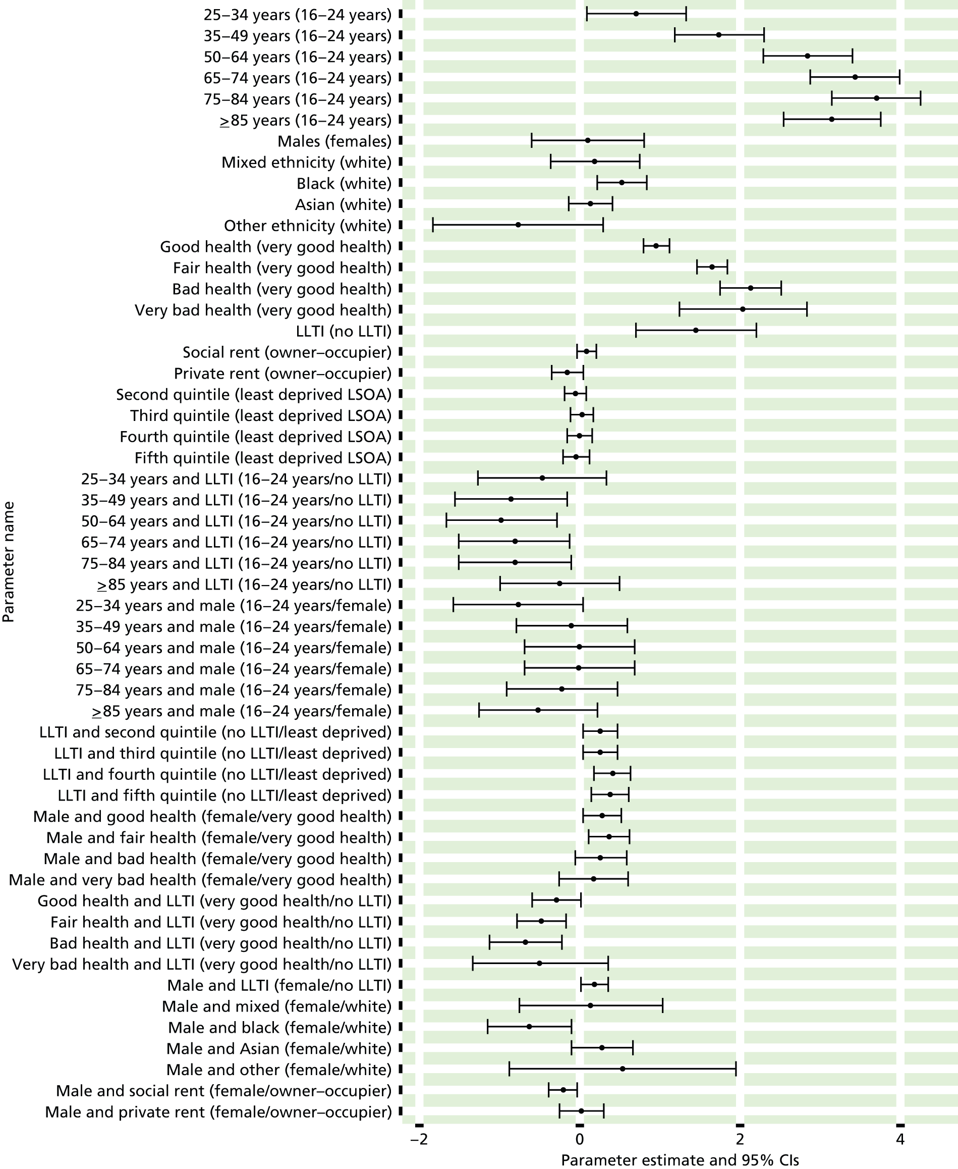
FIGURE 38.
Cardiovascular disease or diabetes as a self-reported LSI: individual estimates and their 95% CIs. (a) MSOAs; (b) LAs; (c) CCGs; and (d) regions (GORs).


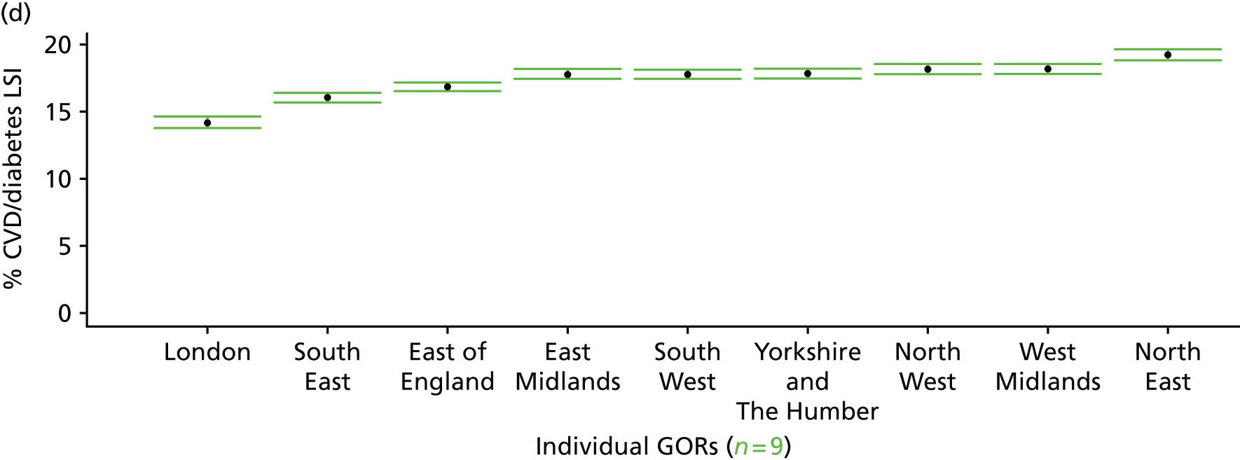
Nurse-measured high blood pressure (Health Survey for England, 2006 and 2009–11)
FIGURE 39.
Nurse-measured high blood pressure: LSOA-level map. Contains Ordnance Survey data © Crown copyright and database right 2012.

Response variable definition, provenance and prediction
These estimates are based on nurse-administered blood pressure readings taken of a subsample of adult respondents to the HSfE. If a valid Omeron reading above 140 mmHg systolic or 90 mmHg diastolic is obtained, the respondent is flagged as having high blood pressure.
The HSfE at this time includes multiple household respondents of all ages. To facilitate comparison with the four different markers of high blood pressure used in this study, the analytical data set is drawn from the most data-restrictive subset of respondents aged ≥ 16 years, namely those for whom we have valid data on blood pressure, doctor diagnoses of illnesses, prescribed drug use and reasons for that use, and self-reported LSI; as well as for the usual set of predictor variables, namely age, sex, ethnicity, general health status, LLTI and tenure and the IMD quintile of their LSOA of residence (n = 19,137). To avoid a potential household-level effect, a single randomly selected adult is drawn from each household, resulting in an analytical data set of 12,103 adults aged ≥ 16 years.
| Age band (years) | Females | Age band (years) | Males | ||||
|---|---|---|---|---|---|---|---|
| Does not have condition | Has condition | % | Does not have condition | Has condition | % | ||
| 16–24 | 488 | 4 | 0.8 | 16–24 | 326 | 22 | 6.3 |
| 25–34 | 955 | 35 | 3.5 | 25–34 | 636 | 92 | 12.6 |
| 35–49 | 1897 | 206 | 9.8 | 35–49 | 1174 | 299 | 20.3 |
| 50–64 | 1417 | 489 | 25.7 | 50–64 | 946 | 488 | 34.0 |
| 65–74 | 461 | 331 | 41.8 | 65–74 | 385 | 249 | 39.3 |
| 75–84 | 318 | 262 | 45.2 | 75–84 | 204 | 153 | 42.9 |
| ≥ 85 | 91 | 89 | 49.4 | ≥ 85 | 42 | 44 | 51.2 |
| Females | 5627 | 1416 | 20.1 | Males | 3713 | 1347 | 26.6 |
| Total (males and females) | 9340 | 2763 | 22.8 | ||||
Model parameters (see below) are applied to microsimulated LSOA-level census data to produce estimates of the number (and proportion) of people expected to have high blood pressure in each age–sex cohort (and overall) in each of the 32,844 English LSOAs. As discussed in the report, bootstrapping is used to derive 95% CIs for these estimates. The bootstrapped LSOA-level prevalence rate estimates are aggregated into a number of higher geographies, namely for MSOAs, LAs, CCGs and GORs, and are then used to calculate 95% CIs for these higher-level estimates. Proportionate attribution is used to restructure the estimates to align with 2001 MSOAs, as well as GP practice populations as defined by the 2011 NHS ADS.
Table 62 summarises how expected prevalence rates vary by age, sex and local deprivation (as measured by the 2010 IMD). There are 6569 LSOAs (with 9,226,227 adults) classified as being in the least deprived quintile; 6568 LSOAs (9,525,344 adults) in the second least deprived quintile; 6568 LSOAs (9,658,444 adults) in the third least deprived quintile; 6568 LSOAs (9,650,576 adults) in the fourth least deprived quintile; and 6568 LSOAs (9,535,167 adults) in the most deprived quintile. Note that, as a general rule, variations in prevalence rates reflect variations in the socioeconomic composition of populations in the different types of LSOA rather than variations in deprivation per se.
| Cohort | Least deprived quintile LSOAs | Second least deprived quintile LSOAs | Third least deprived quintile LSOAs | Fourth least deprived quintile LSOAs | Most deprived quintile LSOAs | All England |
|---|---|---|---|---|---|---|
| Female 16–24 | 0.7 (0.3 to 1.0) | 0.8 (0.4 to 1.2) | 0.7 (0.4 to 1.2) | 0.8 (0.4 to 1.3) | 0.8 (0.4 to 1.4) | 0.8 (0.4 to 1.2) |
| Female 25–34 | 2.9 (2.2 to 3.6) | 3.4 (2.5 to 4.2) | 3.2 (2.4 to 4.1) | 3.4 (2.6 to 4.4) | 3.7 (2.8 to 4.7) | 3.4 (2.6 to 4.2) |
| Female 35–49 | 8.7 (7.5 to 9.8) | 10.1 (8.8 to 11.5) | 9.7 (8.5 to 11.1) | 10.1 (8.7 to 11.4) | 10.7 (9.3 to 12.2) | 9.8 (8.7 to 11.1) |
| Female 50–64 | 23.7 (21.8 to 25.6) | 26.7 (24.8 to 29.3) | 25.9 (24.0 to 28.1) | 26.7 (24.4 to 28.7) | 27.7 (25.2 to 30.0) | 26.0 (24.4 to 27.6) |
| Female 65–74 | 38.3 (35.3 to 41.6) | 42.2 (39.2 to 45.8) | 41.2 (38.2 to 44.8) | 42.3 (39.1 to 45.4) | 43.5 (40.3 to 47.4) | 41.3 (38.9 to 44.3) |
| Female ≥ 75 | 42.2 (38.2 to 45.0) | 46.1 (42.8 to 49.6) | 45.2 (41.2 to 48.4) | 46.5 (42.2 to 49.3) | 47.5 (43.3 to 50.8) | 45.4 (42.0 to 47.9) |
| Females | 19.6 (17.7 to 21.3) | 21.6 (19.9 to 23.8) | 20.0 (18.2 to 22.0) | 18.7 (16.9 to 20.4) | 18.1 (16.3 to 19.9) | 19.6 (18.1 to 21.1) |
| Male 16–24 | 5.1 (3.2 to 6.6) | 5.9 (3.8 to 8.1) | 5.7 (3.7 to 7.7) | 5.9 (3.8 to 7.9) | 6.3 (4.0 to 8.4) | 5.8 (3.7 to 7.6) |
| Male 25–34 | 10.8 (8.5 to 12.5) | 12.4 (9.9 to 14.5) | 11.9 (9.3 to 13.9) | 12.3 (9.8 to 14.0) | 13.1 (10.5 to 15.3) | 12.2 (9.8 to 14.0) |
| Male 35–49 | 18.1 (16.4 to 19.9) | 20.5 (19.0 to 23.2) | 19.8 (18.1 to 22.3) | 20.6 (18.5 to 22.8) | 21.6 (19.6 to 24.0) | 20.1 (18.6 to 22.1) |
| Male 50–64 | 31.6 (29.1 to 33.9) | 35.4 (33.0 to 38.1) | 34.5 (31.9 to 36.5) | 35.4 (32.9 to 37.8) | 36.4 (33.6 to 39.1) | 34.6 (32.7 to 36.7) |
| Male 65–74 | 36.0 (32.5 to 38.6) | 39.9 (36.3 to 43.1) | 38.8 (35.8 to 41.9) | 39.9 (36.1 to 42.4) | 40.9 (36.8 to 44.5) | 39.0 (35.7 to 41.4) |
| Male ≥ 75 | 41.1 (36.2 to 43.8) | 44.9 (40.4 to 48.0) | 43.9 (39.1 to 46.6) | 45.1 (40.2 to 47.5) | 46.1 (40.7 to 48.6) | 44.0 (39.4 to 46.1) |
| Males | 24.2 (21.6 to 26.3) | 26.7 (24.2 to 29.4) | 24.9 (22.3 to 27.2) | 24.0 (21.3 to 26.2) | 24.0 (21.2 to 26.4) | 24.8 (22.4 to 26.7) |
| All | 21.8 (20.5 to 22.8) | 24.1 (22.8 to 25.5) | 22.4 (21.1 to 23.5) | 21.3 (19.8 to 22.3) | 20.9 (19.3 to 22.3) | 22.1 (21.4 to 22.7) |
| Factor (reference group) | Model coefficients | 95% CI | ||
|---|---|---|---|---|
| Estimate | Standard error | 2.5% CI | 97.50% | |
| (Intercept) | –5.11208 | 0.50637 | –6.10457 | –4.11960 |
| Age (16–24 years) | ||||
| 25–34 years | 1.50104 | 0.53088 | 0.46051 | 2.54156 |
| 35–49 years | 2.59737 | 0.50794 | 1.60180 | 3.59294 |
| 50–64 years | 3.73524 | 0.50570 | 2.74407 | 4.72642 |
| 65–74 years | 4.45999 | 0.50831 | 3.46369 | 5.45628 |
| 75–84 years | 4.57290 | 0.51033 | 3.57265 | 5.57315 |
| ≥ 85 years | 4.73457 | 0.52525 | 3.70507 | 5.76407 |
| Sex (females) | ||||
| Males | 2.11807 | 0.54848 | 1.04306 | 3.19309 |
| Ethnicity (white) | ||||
| Mixed | –0.48477 | 0.30604 | –1.08460 | 0.11506 |
| Black | 0.10545 | 0.17183 | –0.23134 | 0.44225 |
| Asian | –0.40020 | 0.14739 | –0.68909 | –0.11130 |
| Other | –0.68594 | 0.48409 | –1.63476 | 0.26288 |
| General health status (very good) | ||||
| Good health | 0.31323 | 0.05727 | 0.20098 | 0.42548 |
| Fair health | 0.38343 | 0.07567 | 0.23511 | 0.53174 |
| Bad health | 0.38388 | 0.11534 | 0.15781 | 0.60995 |
| Very bad health | 0.05267 | 0.19245 | –0.32454 | 0.42988 |
| LLTI (no LTTI) | ||||
| LLTI | –0.15028 | 0.06175 | –0.27132 | –0.02924 |
| Tenure (owner–occupier) | ||||
| Social rent | 0.01231 | 0.07141 | –0.12766 | 0.15229 |
| Private rent or other tenure | –0.02181 | 0.08789 | –0.19409 | 0.15046 |
| LSOA deprivation quintile (least deprived quintile) | ||||
| Second quintile | 0.16318 | 0.06943 | 0.02710 | 0.29927 |
| Third quintile | 0.12825 | 0.07102 | –0.01094 | 0.26745 |
| Fourth quintile | 0.18362 | 0.07473 | 0.03715 | 0.33008 |
| Fifth quintile ( = most deprived quintile) | 0.23982 | 0.08332 | 0.07651 | 0.40312 |
| Interaction effects | ||||
| 25–34 years and male (16–24 years/female) | –0.71995 | 0.58567 | –1.86787 | 0.42796 |
| 35–49 years and male (16–24 years/female) | –1.26567 | 0.55719 | –2.35775 | –0.17358 |
| 50–64 years and male (16–24 years/female) | –1.71331 | 0.55384 | –2.79885 | –0.62778 |
| 65–74 years and male (16–24 years/female) | –2.22788 | 0.55923 | –3.32397 | –1.13179 |
| 75–84 years and male (16–24 years/female) | –2.20247 | 0.56512 | –3.31011 | –1.09483 |
| ≥ 85 years and male (16–24 years/female) | –2.04735 | 0.60839 | –3.23980 | –0.85490 |
FIGURE 40.
Parameter plots: nurse-measured high blood pressure.
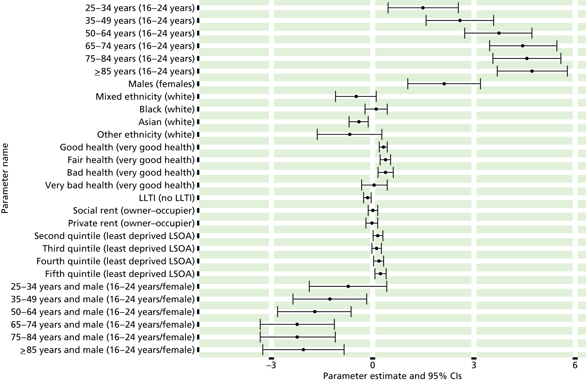
FIGURE 41.
Nurse-measured high blood pressure: individual estimates and their 95% CIs. (a) MSOAs; (b) LAs; (c) CCGs; and (d) region (GORs). BP, blood pressure.


Nurse-measured high blood pressure or using blood pressure medication (Health Survey for England, 2006 and 2009–11)
FIGURE 42.
Nurse-measured high blood pressure or blood pressure drugs: LSOA-level map. Contains Ordnance Survey data © Crown copyright and database right 2012.
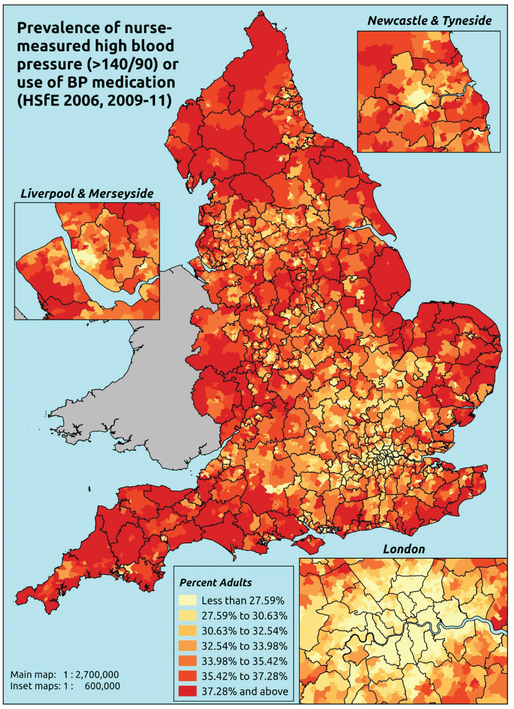
Response variable definition, provenance and prediction
These estimates are based on nurse-administered blood pressure readings and questions about use of prescribed medicines taken of a subsample of adult respondents to the HSfE. If a valid Omeron reading above 140 mmHg systolic or 90 mmHg diastolic is obtained then the respondent is flagged as having high blood pressure. The respondent is flagged as taking medication for high blood pressure only if they are on diuretics, beta-blockers, ACE inhibitors, calcium channel blockers or ‘other blood medication’ which is specifically to control high blood pressure.
The HSfE at this time includes multiple household respondents of all ages. To facilitate comparison with the four different markers of high blood pressure used in this study, the analytical data set is drawn from the most data-restrictive subset of respondents aged ≥ 16 years, namely those for whom we have valid data on blood pressure, doctor diagnoses of illnesses, prescribed drug use and reasons for that use, and self-reported LSI; as well as for the usual set of predictor variables, namely age, sex, ethnicity, general health status, LLTI and tenure and the IMD quintile of their LSOA of residence (n = 19,137). To avoid a potential household-level effect, a single randomly selected adult is drawn from each household, resulting in an analytical data set of 12,103 adults aged ≥ 16 years.
| Age band (years) | Females | Age band (years) | Males | ||||
|---|---|---|---|---|---|---|---|
| Does not have condition | Has condition | % | Does not have condition | Has condition | % | ||
| 16–24 | 488 | 4 | 0.8 | 16–24 | 326 | 22 | 6.3 |
| 25–34 | 951 | 39 | 3.9 | 25–34 | 632 | 96 | 13.2 |
| 35–49 | 1820 | 283 | 13.5 | 35–49 | 1123 | 350 | 23.8 |
| 50–64 | 1182 | 724 | 38.0 | 50–64 | 768 | 666 | 46.4 |
| 65–74 | 286 | 506 | 63.9 | 65–74 | 239 | 395 | 62.3 |
| 75–84 | 148 | 432 | 74.5 | 75–84 | 85 | 272 | 76.2 |
| ≥ 85 | 36 | 144 | 80.0 | ≥ 85 | 23 | 63 | 73.3 |
| Females | 4911 | 2132 | 30.3 | Males | 3196 | 1864 | 36.8 |
| Total (males and females) | 8107 | 3996 | 33.0 | ||||
Model parameters (see below) are applied to microsimulated LSOA-level census data to produce estimates of the number (and proportion) of people expected to have high blood pressure and/or be taking medication for high blood pressure in each age–sex cohort (and overall) in each of the 32,844 English LSOAs. As discussed in the report, bootstrapping is used to derive 95% CIs for these estimates. The bootstrapped LSOA-level prevalence rate estimates are aggregated into a number of higher geographies, namely for MSOAs, LAs, CCGs and GORs, and are then used to calculate 95% CIs for these higher-level estimates. Proportionate attribution is used to restructure the estimates to align with 2001 MSOAs, as well as GP practice populations as defined by the 2011 NHS ADS.
Table 65 summarises how expected prevalence rates vary by age, sex and local deprivation (as measured by the 2010 IMD). There are 6569 LSOAs (with 9,226,227 adults) classified as being in the least deprived quintile; 6568 LSOAs (9,525,344 adults) in the second least deprived quintile; 6568 LSOAs (9,658,444 adults) in the third least deprived quintile; 6568 LSOAs (9,650,576 adults) in the fourth least deprived quintile; and 6568 LSOAs (9,535,167 adults) in the most deprived quintile. Note that, as a general rule, variations in prevalence rates reflect variations in the socioeconomic composition of populations in the different types of LSOA rather than variations in deprivation per se.
| Cohort | Least deprived quintile LSOAs | Second least deprived quintile LSOAs | Third least deprived quintile LSOAs | Fourth least deprived quintile LSOAs | Most deprived quintile LSOAs | All England |
|---|---|---|---|---|---|---|
| Female 16–24 | 0.6 (0.3 to 1.1) | 0.7 (0.4 to 1.2) | 0.7 (0.4 to 1.2) | 0.8 (0.4 to 1.3) | 0.8 (0.4 to 1.4) | 0.7 (0.4 to 1.2) |
| Female 25–34 | 3.0 (2.3 to 3.9) | 3.4 (2.6 to 4.4) | 3.4 (2.5 to 4.4) | 4.0 (2.8 to 5.0) | 4.0 (3.0 to 5.1) | 3.6 (2.7 to 4.6) |
| Female 35–49 | 11.5 (10.5 to 12.8) | 13.0 (12.0 to 14.6) | 13.1 (11.9 to 14.8) | 15.2 (13.6 to 16.8) | 15.4 (13.8 to 17.4) | 13.6 (12.5 to 15.0) |
| Female 50–64 | 35.5 (33.3 to 37.9) | 38.8 (36.6 to 41.6) | 38.9 (36.4 to 41.4) | 43.2 (40.0 to 45.6) | 43.5 (40.3 to 46.3) | 39.7 (37.9 to 41.8) |
| Female 65–74 | 60.6 (57.7 to 63.7) | 63.8 (61.2 to 67.0) | 64.1 (61.2 to 67.1) | 68.0 (64.6 to 70.6) | 68.4 (64.9 to 71.7) | 64.7 (62.3 to 67.3) |
| Female ≥ 75 | 73.6 (70.1 to 76.5) | 76.3 (73.5 to 79.2) | 76.2 (73.7 to 79.3) | 79.1 (75.9 to 81.4) | 78.9 (75.7 to 81.2) | 76.7 (74.0 to 79.1) |
| Females | 30.6 (28.8 to 32.5) | 32.4 (30.7 to 34.5) | 30.9 (29.1 to 32.9) | 30.2 (28.1 to 31.8) | 28.1 (26.1 to 30.0) | 30.4 (28.9 to 32.1) |
| Male 16–24 | 4.7 (3.0 to 6.2) | 5.4 (3.5 to 7.0) | 5.3 (3.3 to 6.9) | 6.1 (3.8 to 7.7) | 6.1 (3.8 to 7.7) | 5.6 (3.6 to 7.1) |
| Male 25–34 | 10.8 (8.8 to 12.6) | 12.1 (9.9 to 14.1) | 11.9 (9.8 to 14.2) | 13.7 (11.0 to 15.4) | 13.8 (11.3 to 15.6) | 12.7 (10.4 to 14.5) |
| Male 35–49 | 20.5 (18.8 to 22.9) | 22.7 (20.8 to 25.3) | 22.9 (21.1 to 25.2) | 26.1 (23.6 to 28.6) | 26.4 (23.8 to 28.9) | 23.7 (22.1 to 26.0) |
| Male 50–64 | 43.5 (40.6 to 46.5) | 47.0 (44.6 to 50.1) | 47.1 (44.5 to 50.3) | 51.5 (48.6 to 54.1) | 51.8 (48.7 to 54.9) | 48.0 (45.6 to 50.2) |
| Male 65–74 | 59.2 (55.3 to 62.8) | 62.4 (59.0 to 65.9) | 62.6 (58.8 to 66.1) | 66.6 (63.0 to 69.0) | 66.7 (62.8 to 69.5) | 63.2 (59.9 to 66.0) |
| Male ≥ 75 | 73.8 (69.5 to 76.8) | 76.3 (72.3 to 79.2) | 76.2 (72.4 to 79.5) | 79.1 (74.9 to 81.7) | 79.0 (75.1 to 81.4) | 76.6 (73.1 to 79.4) |
| Males | 34.6 (32.0 to 37.2) | 36.5 (34.0 to 39.2) | 34.7 (32.2 to 37.4) | 34.8 (31.9 to 37.0) | 33.3 (30.4 to 35.6) | 34.8 (32.4 to 37.0) |
| All | 32.5 (31.3 to 33.8) | 34.4 (33.3 to 35.7) | 32.7 (31.5 to 34.1) | 32.4 (30.7 to 33.3) | 30.6 (28.9 to 31.8) | 32.5 (31.8 to 33.2) |
| Factor (reference group) | Model coefficients | 95% CI | ||
|---|---|---|---|---|
| Estimate | Standard error | 2.5% CI | 97.50% | |
| (Intercept) | –5.33966 | 0.50643 | –6.33227 | –4.34705 |
| Age (16–24 years) | ||||
| 25–34 years | 1.59344 | 0.52833 | 0.55791 | 2.62898 |
| 35–49 years | 2.93198 | 0.50682 | 1.93861 | 3.92534 |
| 50–64 years | 4.26815 | 0.50533 | 3.27771 | 5.25860 |
| 65–74 years | 5.31077 | 0.50876 | 4.31361 | 6.30794 |
| 75–84 years | 5.71532 | 0.51247 | 4.71088 | 6.71976 |
| ≥ 85 years | 6.02071 | 0.53736 | 4.96748 | 7.07394 |
| Sex (females) | ||||
| Males | 2.14063 | 0.54878 | 1.06503 | 3.21623 |
| Ethnicity (white) | ||||
| Mixed | –0.24575 | 0.26476 | –0.76469 | 0.27319 |
| Black | 0.33107 | 0.16337 | 0.01085 | 0.65128 |
| Asian | –0.15877 | 0.13003 | –0.41363 | 0.09609 |
| Other | –0.35014 | 0.40043 | –1.13499 | 0.43470 |
| General health status (very good) | ||||
| Good health | 0.57021 | 0.05553 | 0.46138 | 0.67904 |
| Fair health | 0.85827 | 0.07408 | 0.71307 | 1.00348 |
| Bad health | 1.01386 | 0.11437 | 0.78969 | 1.23802 |
| Very bad health | 0.75303 | 0.18102 | 0.39824 | 1.10782 |
| LLTI (no LTTI) | ||||
| LLTI | –0.09072 | 0.06061 | –0.20952 | 0.02807 |
| Tenure (owner–occupier) | ||||
| Social rent | 0.05895 | 0.07063 | –0.07948 | 0.19737 |
| Private rent or other tenure | –0.09328 | 0.08527 | –0.26041 | 0.07385 |
| LSOA deprivation quintile (least deprived quintile) | ||||
| Second quintile | 0.11757 | 0.06769 | –0.01511 | 0.25024 |
| Third quintile | 0.09118 | 0.06893 | –0.04392 | 0.22627 |
| Fourth quintile | 0.23073 | 0.07249 | 0.08866 | 0.37281 |
| Fifth quintile ( = most deprived quintile) | 0.18176 | 0.08124 | 0.02253 | 0.34099 |
| Interaction effects | ||||
| 25–34 years and male (16–24 years/female) | –0.75694 | 0.58324 | –1.90009 | 0.38621 |
| 35–49 years and male (16–24 years/female) | –1.43376 | 0.55600 | –2.52352 | –0.34400 |
| 50–64 years and male (16–24 years/female) | –1.79466 | 0.55349 | –2.87950 | –0.70981 |
| 65–74 years and male (16–24 years/female) | –2.21634 | 0.56010 | –3.31414 | –1.11854 |
| 75–84 years and male (16–24 years/female) | –1.99052 | 0.57115 | –3.10998 | –0.87107 |
| ≥ 85 years and male (16–24 years/female) | –2.48169 | 0.63044 | –3.71736 | –1.24603 |
FIGURE 43.
Parameter plots: nurse-measured high blood pressure or blood pressure drugs.
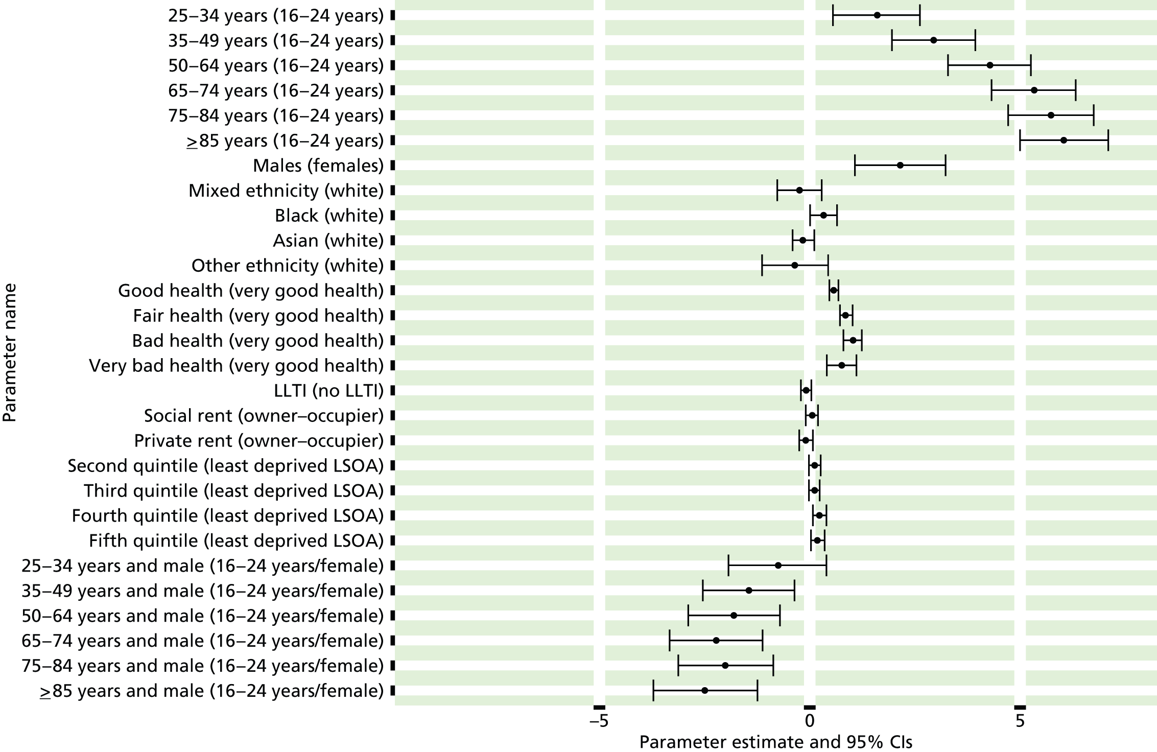
FIGURE 44.
Nurse-measured high blood pressure or blood pressure drugs: individual estimates and their 95% CIs. (a) MSOAs; (b) LAs; (c) CCGs; and (d) regions (GORs).


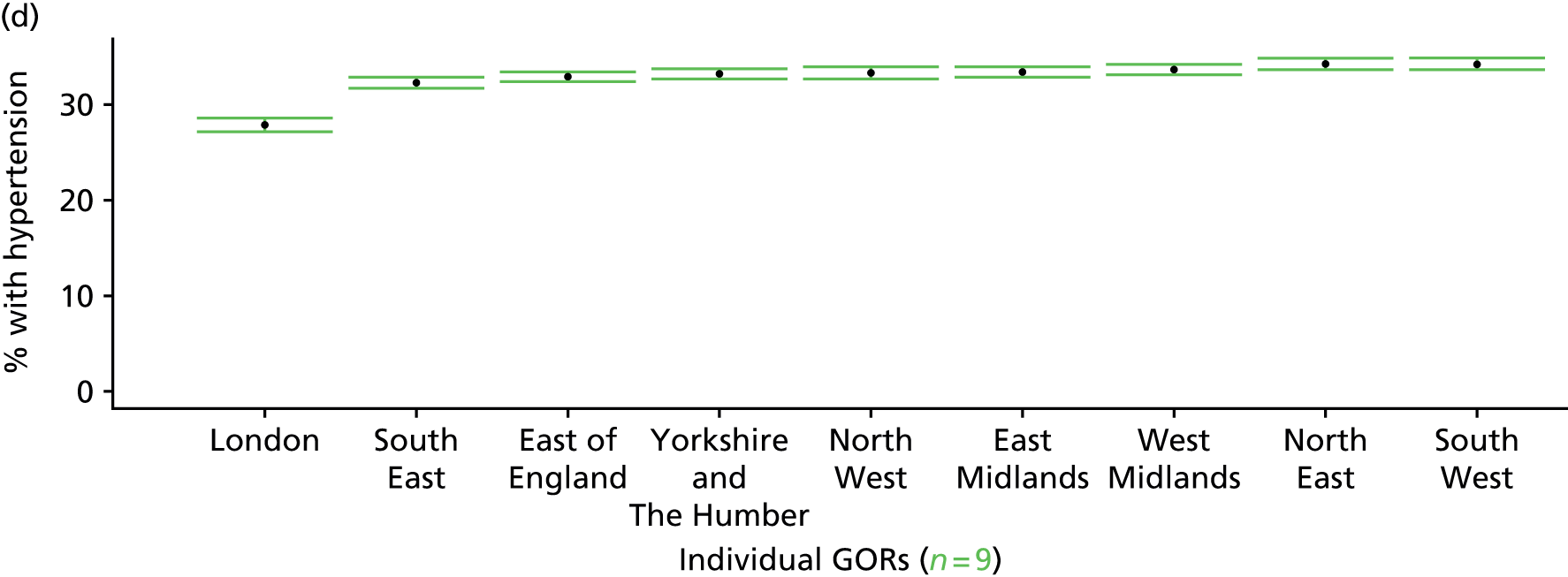
Clinical evidence of current treated or untreated high blood pressure (Health Survey for England, 2006 and 2009–11)
FIGURE 45.
Clinical evidence of treated/untreated high blood pressure: LSOA-level map. Contains Ordnance Survey data © Crown copyright and database right 2012.
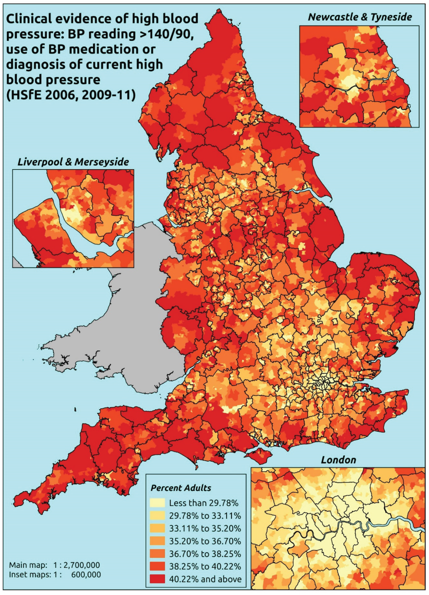
Response variable definition, provenance and prediction
These estimates are based on HSfE nurse-administered blood pressure readings, questions about the use of prescribed medicines, and questions about current doctor diagnosis of high blood pressure. If a valid Omeron reading above 140 mmHg systolic or 90 mmHg diastolic is obtained, the respondent is flagged as having high blood pressure. The respondent is flagged as taking medication for high blood pressure only if they are on diuretics, beta-blockers, ACE inhibitors, calcium channel blockers or ‘other blood medication’ which is specifically to control high blood pressure.
The HSfE at this time includes multiple household respondents of all ages. To facilitate comparison with the four different markers of high blood pressure used in this study, the analytical data set is drawn from the most data-restrictive subset of respondents aged ≥ 16 years, namely those for whom we have valid data on blood pressure, doctor diagnoses of illnesses, prescribed drug use and reasons for that use, and self-reported LSI; as well as for the usual set of predictor variables, namely age, sex, ethnicity, general health status, LLTI and tenure and the IMD quintile of their LSOA of residence (n = 19,137). To avoid a potential household-level effect, a single randomly selected adult is drawn from each household, resulting in an analytical data set of 12,103 adults aged ≥ 16 years.
| Age band (years) | Females | Age band (years) | Males | ||||
|---|---|---|---|---|---|---|---|
| Does not have condition | Has condition | % | Does not have condition | Has condition | % | ||
| 16–24 | 485 | 7 | 1.4 | 16–24 | 324 | 24 | 6.9 |
| 25–34 | 939 | 51 | 5.2 | 25–34 | 617 | 111 | 15.2 |
| 35–49 | 1785 | 318 | 15.1 | 35–49 | 1088 | 385 | 26.1 |
| 50–64 | 1130 | 776 | 40.7 | 50–64 | 705 | 729 | 50.8 |
| 65–74 | 270 | 522 | 65.9 | 65–74 | 211 | 423 | 66.7 |
| 75–84 | 117 | 463 | 79.8 | 75–84 | 80 | 277 | 77.6 |
| ≥ 85 | 28 | 152 | 84.4 | ≥ 85 | 18 | 68 | 79.1 |
| Females | 4754 | 2289 | 32.5 | Males | 3043 | 2017 | 39.9 |
| Total (males and females) | 7797 | 4306 | 35.6 | ||||
Model parameters (see below) are applied to microsimulated LSOA-level census data to produce estimates of the number (and proportion) of people expected to have high blood pressure and/or be taking medication for high blood pressure and/or who report that they are currently diagnosed with high blood pressure in each age–sex cohort (and overall) in each of the 32,844 English LSOAs. As discussed in the report, bootstrapping is used to derive 95% CIs for these estimates. The bootstrapped LSOA-level prevalence rate estimates are aggregated into a number of higher geographies, namely for MSOAs, LAs, CCGs and GORs, and are then used to calculate 95% CIs for these higher-level estimates. Proportionate attribution is used to restructure the estimates to align with 2001 MSOAs, as well as GP practice populations as defined by the 2011 NHS ADS.
Table 68 summarises how expected prevalence rates vary by age, sex and local deprivation (as measured by the 2010 IMD). There are 6569 LSOAs (with 9,226,227 adults) classified as being in the least deprived quintile; 6568 LSOAs (9,525,344 adults) in the second least deprived quintile; 6568 LSOAs (9,658,444 adults) in the third least deprived quintile; 6568 LSOAs (9,650,576 adults) in the fourth least deprived quintile; and 6568 LSOAs (9,535,167 adults) in the most deprived quintile. Note that, as a general rule, variations in prevalence rates reflect variations in the socioeconomic composition of populations in the different types of LSOA rather than variations in deprivation per se.
| Cohort | Least deprived quintile LSOAs | Second least deprived quintile LSOAs | Third least deprived quintile LSOAs | Fourth least deprived quintile LSOAs | Most deprived quintile LSOAs | All England |
|---|---|---|---|---|---|---|
| Female 16–24 | 1.1 (0.6 to 1.8) | 1.2 (0.7 to 2.0) | 1.2 (0.7 to 2.0) | 1.4 (0.8 to 2.3) | 1.3 (0.8 to 2.2) | 1.3 (0.7 to 2.1) |
| Female 25–34 | 3.9 (3.0 to 5.0) | 4.2 (3.2 to 5.2) | 4.5 (3.4 to 5.5) | 5.2 (3.9 to 6.3) | 5.0 (4.0 to 6.2) | 4.7 (3.7 to 5.7) |
| Female 35–49 | 13.0 (11.9 to 14.2) | 14.0 (12.9 to 15.7) | 15.1 (13.7 to 16.7) | 17.2 (15.4 to 18.8) | 17.1 (15.3 to 18.9) | 15.3 (14.2 to 16.6) |
| Female 50–64 | 38.4 (36.0 to 40.8) | 40.5 (38.1 to 43.3) | 42.5 (40.1 to 45.2) | 46.7 (43.7 to 49.1) | 46.6 (42.8 to 48.8) | 42.6 (40.6 to 44.5) |
| Female 65–74 | 63.1 (60.3 to 66.4) | 65.3 (62.3 to 68.6) | 67.0 (64.1 to 69.7) | 70.7 (67.5 to 73.3) | 70.6 (67.2 to 73.3) | 67.0 (64.5 to 69.6) |
| Female ≥ 75 | 79.6 (76.8 to 82.4) | 81.0 (78.1 to 83.7) | 82.1 (79.4 to 84.5) | 84.3 (81.5 to 86.3) | 83.6 (80.8 to 85.7) | 82.0 (79.6 to 84.4) |
| Females | 33.0 (31.2 to 35.0) | 34.1 (32.2 to 36.2) | 33.5 (31.7 to 35.5) | 32.6 (30.5 to 34.3) | 30.1 (28.0 to 31.8) | 32.7 (31.1 to 34.3) |
| Male 16–24 | 5.2 (3.6 to 7.1) | 5.5 (3.9 to 7.5) | 5.9 (4.0 to 7.9) | 6.7 (4.6 to 9.0) | 6.4 (4.5 to 8.5) | 6.0 (4.1 to 8.0) |
| Male 25–34 | 12.8 (10.3 to 14.7) | 13.6 (11.0 to 15.8) | 14.1 (11.3 to 15.8) | 15.8 (12.8 to 17.8) | 15.5 (12.4 to 17.5) | 14.6 (11.8 to 16.3) |
| Male 35–49 | 22.8 (20.9 to 24.7) | 24.2 (22.5 to 26.6) | 25.7 (23.8 to 28.1) | 28.8 (25.8 to 31.2) | 28.6 (25.9 to 30.8) | 26.0 (24.3 to 27.9) |
| Male 50–64 | 48.1 (45.4 to 51.0) | 50.4 (48.2 to 53.7) | 52.5 (50.0 to 55.1) | 56.7 (53.4 to 59.1) | 56.3 (53.6 to 58.9) | 52.6 (50.3 to 54.7) |
| Male 65–74 | 64.1 (60.7 to 67.0) | 66.3 (63.2 to 69.4) | 68.0 (64.6 to 70.8) | 71.6 (67.8 to 74.0) | 71.3 (67.5 to 73.5) | 67.9 (64.8 to 70.3) |
| Male ≥ 75 | 77.1 (72.1 to 79.8) | 78.7 (73.9 to 81.5) | 79.8 (75.2 to 81.9) | 82.2 (77.6 to 84.4) | 81.6 (77.1 to 83.8) | 79.6 (75.1 to 81.7) |
| Males | 37.7 (35.0 to 40.1) | 38.8 (36.3 to 41.5) | 38.1 (35.5 to 40.5) | 37.8 (34.7 to 40.1) | 35.8 (32.9 to 38.0) | 37.6 (35.2 to 39.6) |
| All | 35.3 (34.1 to 36.5) | 36.3 (35.3 to 37.7) | 35.8 (34.7 to 36.9) | 35.1 (33.5 to 36.0) | 32.9 (31.3 to 33.9) | 35.1 (34.3 to 35.6) |
| Factor (reference group) | Model coefficients | 95% CI | ||
|---|---|---|---|---|
| Estimate | Standard error | 2.5% CI | 97.50% | |
| (Intercept) | –4.81484 | 0.38630 | –5.57199 | –4.05768 |
| Age (16–24 years) | ||||
| 25–34 years | 1.30475 | 0.40740 | 0.50626 | 2.10325 |
| 35–49 years | 2.47935 | 0.38642 | 1.72197 | 3.23673 |
| 50–64 years | 3.77859 | 0.38487 | 3.02425 | 4.53293 |
| 65–74 years | 4.78492 | 0.38968 | 4.02115 | 5.54868 |
| 75–84 years | 5.37398 | 0.39649 | 4.59686 | 6.15111 |
| ≥ 85 years | 5.67036 | 0.43534 | 4.81709 | 6.52363 |
| Sex (females) | ||||
| Males | 1.69613 | 0.43631 | 0.84096 | 2.55131 |
| Ethnicity (white) | ||||
| Mixed | –0.40990 | 0.26519 | –0.92967 | 0.10987 |
| Black | 0.23751 | 0.16261 | –0.08121 | 0.55623 |
| Asian | –0.20607 | 0.12745 | –0.45588 | 0.04373 |
| Other | –0.39027 | 0.38834 | –1.15142 | 0.37088 |
| General health status (very good) | ||||
| Good health | 0.61759 | 0.05480 | 0.51017 | 0.72500 |
| Fair health | 0.97254 | 0.07387 | 0.82775 | 1.11733 |
| Bad health | 1.15673 | 0.11543 | 0.93048 | 1.38297 |
| Very bad health | 1.01538 | 0.18359 | 0.65555 | 1.37522 |
| LLTI (no LTTI) | ||||
| LLTI | 0.04965 | 0.07516 | –0.09766 | 0.19695 |
| Tenure (owner–occupier) | ||||
| Social rent | 0.11767 | 0.07065 | –0.02080 | 0.25615 |
| Private rent or other tenure | –0.11081 | 0.08350 | –0.27448 | 0.05285 |
| LSOA deprivation quintile (least deprived quintile) | ||||
| Second quintile | 0.05970 | 0.06738 | –0.07236 | 0.19176 |
| Third quintile | 0.10009 | 0.06836 | –0.03390 | 0.23407 |
| Fourth quintile | 0.21795 | 0.07198 | 0.07686 | 0.35904 |
| Fifth quintile ( = most deprived quintile) | 0.11906 | 0.08067 | –0.03906 | 0.27719 |
| Interaction effects | ||||
| 25–34 years and male (16–24 years/female) | –0.38531 | 0.47116 | –1.30878 | 0.53816 |
| 35–49 years and male (16–24 years/female) | –0.95171 | 0.44478 | –1.82349 | –0.07993 |
| 50–64 years and male (16–24 years/female) | –1.23706 | 0.44254 | –2.10444 | –0.36967 |
| 65–74 years and male (16–24 years/female) | –1.61142 | 0.45175 | –2.49686 | –0.72598 |
| 75–84 years and male (16–24 years/female) | –1.68679 | 0.46804 | –2.60414 | –0.76944 |
| ≥ 85 years and male (16–24 years/female) | –1.92701 | 0.55456 | –3.01395 | –0.84008 |
| Male and LLTI (female/no LLTI) | –0.15714 | 0.10192 | –0.35690 | 0.04262 |
FIGURE 46.
Parameter plots: clinical evidence of treated/untreated high blood pressure.
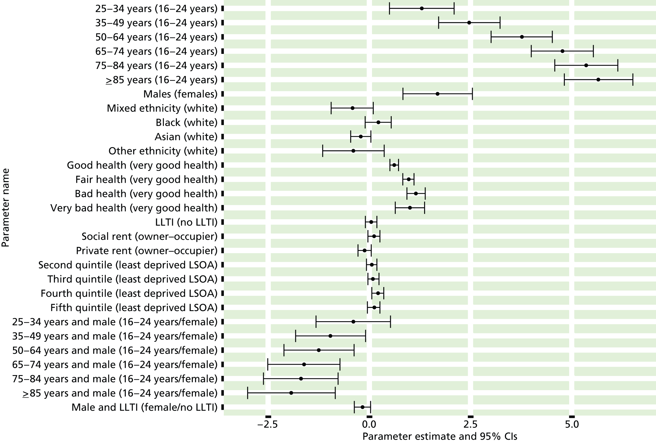
FIGURE 47.
Clinical evidence of treated/untreated high blood pressure: individual estimates and their 95% CIs. (a) MSOAs; (b) LAs; (c) CCGs; and (d) regions (GORs).


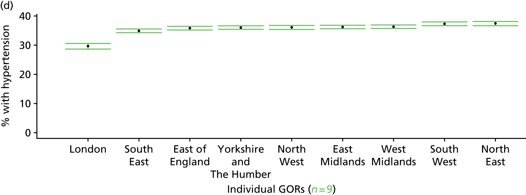
History of treated/untreated high blood pressure (Health Survey for England, 2006 and 2009–11)
FIGURE 48.
History of treated/untreated high blood pressure: LSOA-level map. Contains Ordnance Survey data © Crown copyright and database right 2012.
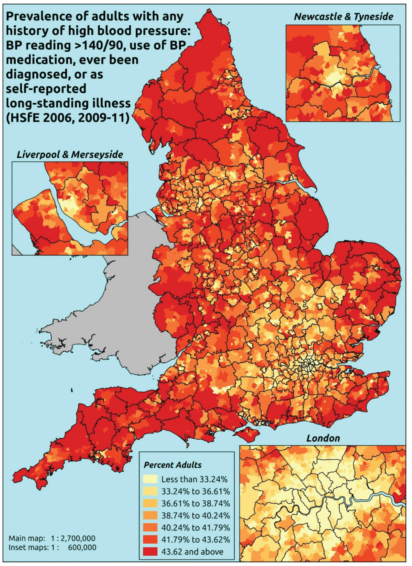
Response variable definition, provenance and prediction
These estimates are based on HSfE nurse-administered blood pressure readings, questions about the use of prescribed medicines, questions about ever having been diagnosed with high blood pressure, and self-reported LSI. If a valid Omeron reading above 140 mmHg systolic or 90 mmHg diastolic is obtained, the respondent is flagged as having high blood pressure. The respondent is flagged as taking medication for high blood pressure only if they are on diuretics, beta-blockers, ACE inhibitors, calcium channel blockers or ‘other blood medication’ which is specifically to control high blood pressure.
The HSfE at this time includes multiple household respondents of all ages. To facilitate comparison with the four different markers of high blood pressure used in this study, the analytical data set is drawn from the most data-restrictive subset of respondents aged ≥ 16 years, namely those for whom we have valid data on blood pressure, doctor diagnoses of illnesses, prescribed drug use and reasons for that use, and self-reported long-standing illness; as well as for the usual set of predictor variables, namely age, sex, ethnicity, general health status, LLTI and tenure and the IMD quintile of their LSOA of residence (n = 19,137). To avoid a potential household-level effect, a single randomly selected adult is drawn from each household, resulting in an analytical data set of 12,103 adults aged ≥ 16 years.
| Age band | Females | Age band | Males | ||||
|---|---|---|---|---|---|---|---|
| Does not have condition | Has condition | % | Does not have condition | Has condition | % | ||
| 16–24 | 472 | 20 | 4.1 | 16–24 | 317 | 31 | 8.9 |
| 25–34 | 886 | 104 | 10.5 | 25–34 | 588 | 140 | 19.2 |
| 35–49 | 1682 | 421 | 20.0 | 35–49 | 1028 | 445 | 30.2 |
| 50–64 | 1044 | 862 | 45.2 | 50–64 | 647 | 787 | 54.9 |
| 65–74 | 254 | 538 | 67.9 | 65–74 | 196 | 438 | 69.1 |
| 75–84 | 105 | 475 | 81.9 | 75–84 | 76 | 281 | 78.7 |
| ≥ 85 | 26 | 154 | 85.6 | ≥ 85 | 17 | 69 | 80.2 |
| Females | 4469 | 2574 | 36.5 | Males | 2869 | 2191 | 43.3 |
| Total (males and females) | 7338 | 4765 | 39.4 | ||||
Model parameters (see below) are applied to microsimulated LSOA-level census data to produce estimates of the number (and proportion) of people expected to have high blood pressure and/or be taking medication for high blood pressure and/or who have ever been diagnosed with high blood pressure and/or who report high blood pressure as a LSI in each age–sex cohort (and overall) in each of the 32,844 English LSOAs. As discussed in the report, bootstrapping is used to derive 95% CIs for these estimates. The bootstrapped LSOA-level prevalence rate estimates are aggregated into a number of higher geographies, namely for MSOAs, LAs, CCGs and GORs, and are then used to calculate 95% CIs for these higher-level estimates. Proportionate attribution is used to restructure the estimates to align with 2001 MSOAs, as well as GP practice populations as defined by the 2011 NHS ADS.
Table 71 summarises how expected prevalence rates vary by age, sex and local deprivation (as measured by the 2010 IMD). There are 6569 LSOAs (with 9,226,227 adults) classified as being in the least deprived quintile; 6568 LSOAs (9,525,344 adults) in the second least deprived quintile; 6568 LSOAs (9,658,444 adults) in the third least deprived quintile; 6568 LSOAs (9,650,576 adults) in the fourth least deprived quintile; and 6568 LSOAs (9,535,167 adults) in the most deprived quintile. Note that, as a general rule, variations in prevalence rates reflect variations in the socioeconomic composition of populations in the different types of LSOA rather than variations in deprivation per se.
| Cohort | Least deprived quintile LSOAs | Second least deprived quintile LSOAs | Third least deprived quintile LSOAs | Fourth least deprived quintile LSOAs | Most deprived quintile LSOAs | All England |
|---|---|---|---|---|---|---|
| Female 16–24 | 2.9 (1.9 to 4.4) | 3.2 (2.3 to 4.7) | 3.4 (2.3 to 4.9) | 4.0 (2.8 to 5.7) | 4.0 (2.8 to 5.9) | 3.6 (2.5 to 5.2) |
| Female 25–34 | 8.0 (6.9 to 9.2) | 8.6 (7.3 to 9.8) | 8.9 (7.8 to 10.5) | 10.6 (9.0 to 11.9) | 10.4 (9.0 to 12.0) | 9.5 (8.2 to 10.8) |
| Female 35–49 | 17.0 (15.6 to 18.9) | 18.5 (17.1 to 20.6) | 19.6 (18.3 to 21.6) | 22.9 (20.9 to 24.8) | 22.9 (21.2 to 25.2) | 20.2 (18.9 to 21.8) |
| Female 50–64 | 42.2 (39.9 to 44.7) | 44.8 (42.6 to 47.6) | 46.7 (44.5 to 49.5) | 52.1 (49.3 to 54.6) | 53.0 (49.8 to 56.2) | 47.4 (45.6 to 49.3) |
| Female 65–74 | 64.8 (61.4 to 68.0) | 67.3 (64.4 to 70.7) | 68.8 (66.0 to 71.9) | 73.2 (70.5 to 76.0) | 73.6 (70.7 to 76.4) | 69.1 (66.7 to 71.9) |
| Female ≥ 75 | 80.7 (77.6 to 83.5) | 82.1 (79.6 to 84.7) | 82.9 (80.2 to 85.4) | 85.5 (82.8 to 87.5) | 85.2 (82.6 to 87.5) | 83.1 (80.7 to 85.4) |
| Females | 36.1 (34.1 to 38.3) | 37.4 (35.5 to 39.8) | 36.9 (35.0 to 39.1) | 36.8 (34.7 to 38.9) | 34.7 (32.6 to 37.1) | 36.4 (34.8 to 38.2) |
| Male 16–24 | 7.0 (5.1 to 8.8) | 7.7 (5.4 to 9.5) | 8.1 (5.9 to 10.1) | 9.5 (6.9 to 11.9) | 9.6 (7.1 to 11.9) | 8.5 (6.3 to 10.6) |
| Male 25–34 | 15.8 (13.2 to 17.8) | 16.9 (14.2 to 18.5) | 17.4 (14.6 to 19.8) | 19.9 (16.8 to 21.7) | 19.7 (16.7 to 21.8) | 18.3 (15.8 to 20.0) |
| Male 35–49 | 26.0 (23.9 to 28.2) | 27.9 (25.8 to 29.9) | 29.2 (27.2 to 31.6) | 33.3 (30.9 to 35.3) | 33.4 (30.6 to 36.3) | 30.0 (28.3 to 31.8) |
| Male 50–64 | 51.3 (49.1 to 54.1) | 54.0 (51.8 to 57.1) | 56.1 (53.8 to 59.3) | 61.2 (58.7 to 63.9) | 61.8 (59.3 to 64.8) | 56.6 (54.7 to 58.8) |
| Male 65–74 | 66.1 (62.5 to 69.0) | 68.5 (65.1 to 71.3) | 70.1 (66.8 to 73.1) | 74.3 (70.9 to 76.8) | 74.5 (71.0 to 77.3) | 70.3 (67.2 to 72.7) |
| Male ≥ 75 | 77.2 (72.6 to 80.0) | 78.9 (74.7 to 81.6) | 79.7 (75.3 to 82.7) | 82.6 (78.8 to 84.8) | 82.4 (78.5 to 85.1) | 79.9 (76.0 to 82.5) |
| Males | 40.2 (37.6 to 42.7) | 41.6 (39.0 to 44.0) | 40.9 (38.3 to 43.6) | 41.5 (38.7 to 43.7) | 39.9 (37.0 to 42.5) | 40.8 (38.5 to 42.9) |
| All | 38.1 (36.7 to 39.3) | 39.5 (38.2 to 40.6) | 38.8 (37.7 to 40.2) | 39.1 (37.5 to 40.1) | 37.2 (35.8 to 38.7) | 38.5 (37.9 to 39.2) |
| Factor (reference group) | Model coefficients | 95% CI | ||
|---|---|---|---|---|
| Estimate | Standard error | 2.5% CI | 97.50% | |
| (Intercept) | –3.74956 | 0.23697 | –4.21402 | –3.28511 |
| Age (16–24 years) | ||||
| 25–34 years | 1.00757 | 0.25171 | 0.51421 | 1.50093 |
| 35–49 years | 1.74921 | 0.23634 | 1.28599 | 2.21243 |
| 50–64 years | 2.88916 | 0.23513 | 2.42831 | 3.35002 |
| 65–74 years | 3.80048 | 0.24332 | 3.32357 | 4.27738 |
| 75–84 years | 4.43109 | 0.25536 | 3.93059 | 4.93159 |
| ≥ 85 years | 4.68205 | 0.3149 | 4.06484 | 5.29926 |
| Sex (females) | ||||
| Males | 0.88448 | 0.29709 | 0.30219 | 1.46678 |
| Ethnicity (white) | ||||
| Mixed | –0.33233 | 0.23935 | –0.80146 | 0.13681 |
| Black | 0.03827 | 0.15556 | –0.26662 | 0.34316 |
| Asian | –0.27799 | 0.11938 | –0.51198 | –0.04400 |
| Other | –0.29365 | 0.34990 | –0.97946 | 0.39216 |
| General health status (very good) | ||||
| Good health | 0.62125 | 0.05211 | 0.51910 | 0.72339 |
| Fair health | 0.94170 | 0.07148 | 0.80160 | 1.08180 |
| Bad health | 1.16019 | 0.11438 | 0.93601 | 1.38438 |
| Very bad health | 1.15571 | 0.18565 | 0.79183 | 1.51958 |
| LLTI (no LTTI) | ||||
| LLTI | 0.05996 | 0.05897 | –0.05562 | 0.17553 |
| Tenure (owner–occupier) | ||||
| Social rent | 0.08633 | 0.06831 | –0.04755 | 0.22022 |
| Private rent or other tenure | –0.11064 | 0.07780 | –0.26313 | 0.04185 |
| LSOA deprivation quintile (least deprived quintile) | ||||
| Second quintile | 0.07032 | 0.06523 | –0.05752 | 0.19816 |
| Third quintile | 0.10931 | 0.06611 | –0.02027 | 0.23889 |
| Fourth quintile | 0.26470 | 0.06949 | 0.12851 | 0.40089 |
| Fifth quintile ( = most deprived quintile) | 0.19392 | 0.07739 | 0.04224 | 0.34560 |
| Interaction effects | ||||
| 25–34 years and male (16–24 years/female) | –0.08904 | 0.32904 | –0.73395 | 0.55587 |
| 35–49 years and male (16–24 years/female) | –0.31453 | 0.30767 | –0.91755 | 0.28850 |
| 50–64 years and male (16–24 years/female) | –0.49373 | 0.30569 | –1.09288 | 0.10542 |
| 65–74 years and male (16–24 years/female) | –0.83284 | 0.31936 | –1.45879 | –0.20689 |
| 75–84 years and male (16–24 years/female) | –1.00959 | 0.34271 | –1.68130 | –0.33787 |
| ≥ 85 years and male (16–24 years/female) | –1.20249 | 0.45796 | –2.10009 | –0.30489 |
FIGURE 49.
Parameter plots: history of treated/untreated high blood pressure.
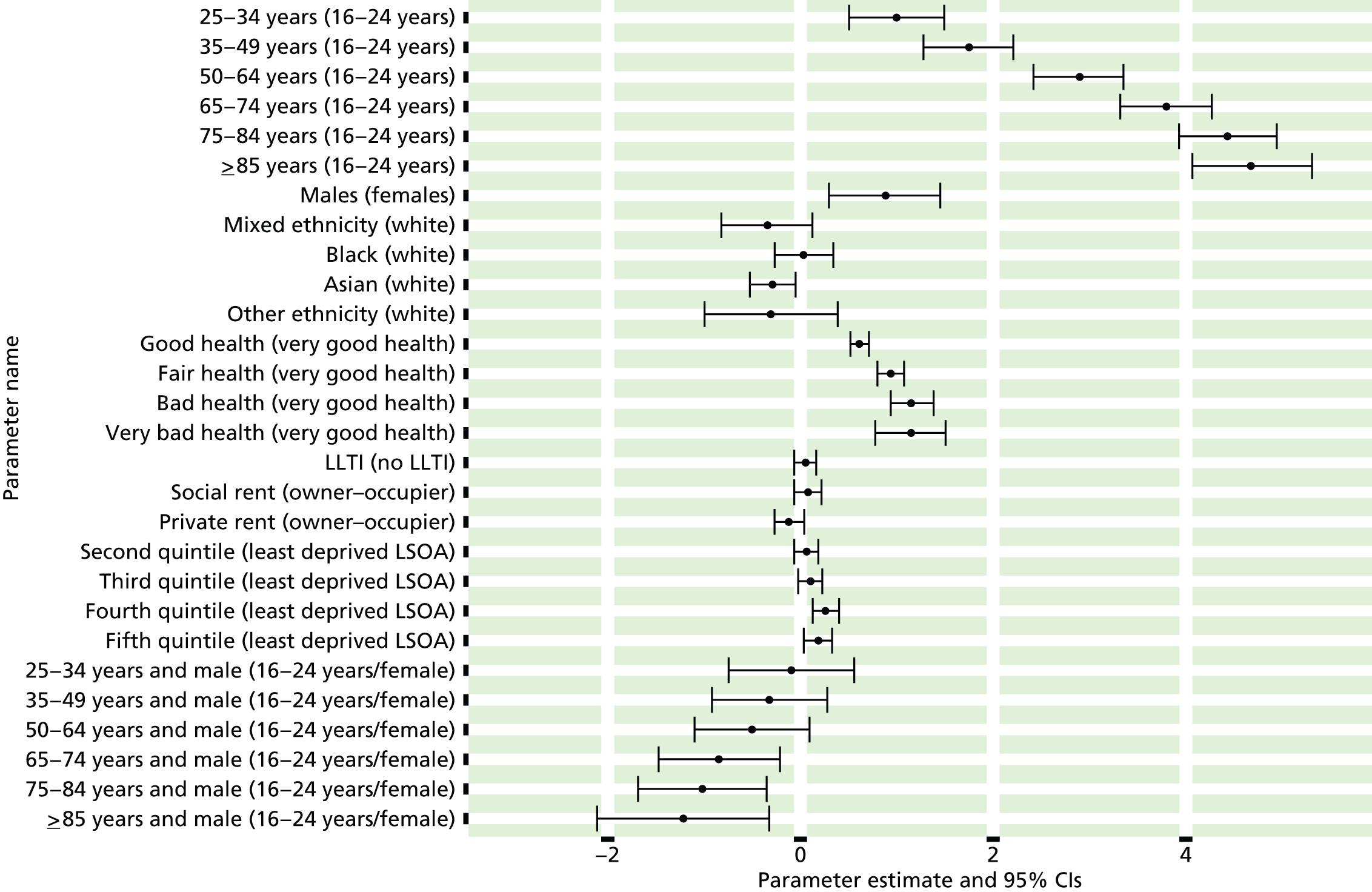
FIGURE 50.
History of treated/untreated high blood pressure: individual estimates and their 95% CIs. (a) MSOAs; (b) LAs; (c) CCGs; and (d) regions (GORs).


Coronary heart disease (angina or myocardial infarction) symptoms (Health Survey for England, 2006 and 2011)
FIGURE 51.
Coronary heart disease (angina or MI) symptoms: LSOA-level map. Contains Ordnance Survey data © Crown copyright and database right 2012.
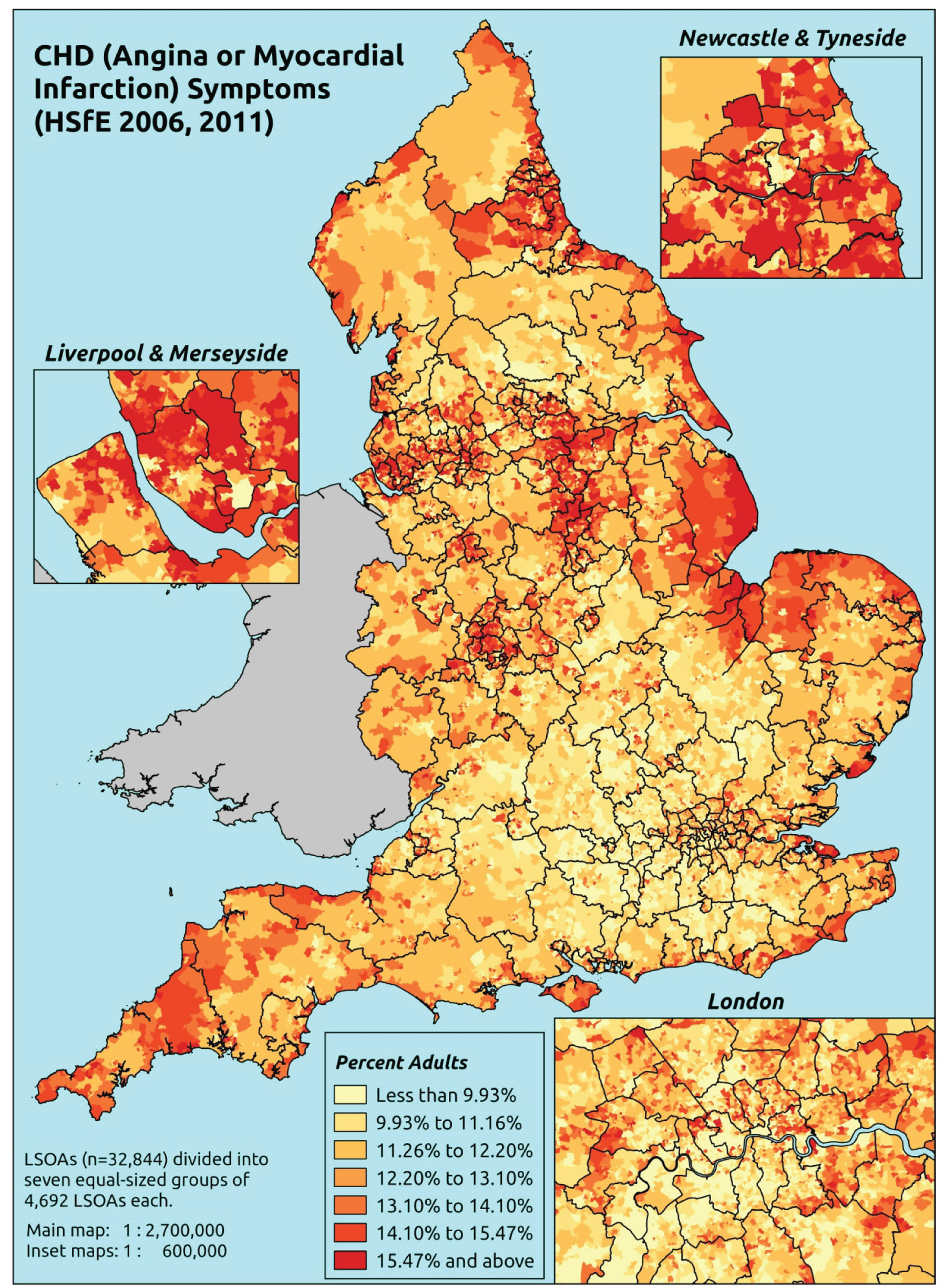
Response variable definition, provenance and prediction
These estimates are based on respondents to the HSfE reporting that they had (a) ever had chest pain in sternum, sternum lower or anterior lower chest and in the left arm (angina symptoms) and/or (b) ever had a severe pain across the front of their chest lasting half an hour or more (possible MI).
The HSfE at this time includes multiple household respondents of all ages. The analytical data set is drawn from the subset of respondents aged ≥ 16 years for whom data are available across all model response and predictor variables, namely whether or not they responded to questions on angina and MI symptoms, whether or not they provided responses to questions on age, sex, ethnicity, general health status, LLTI and tenure, and whether or not information is available on the IMD quintile of their LSOA of residence (n = 20,965). To avoid a potential household-level effect, a single randomly selected adult is drawn from each household, resulting in an analytical data set of 13,835 adults aged ≥ 16 years.
| Age band (years) | Females | Age band (years) | Males | ||||
|---|---|---|---|---|---|---|---|
| Does not have condition | Has condition | % | Does not have condition | Has condition | % | ||
| 16–24 | 591 | 17 | 2.8 | 16–24 | 414 | 10 | 2.4 |
| 25–34 | 1153 | 58 | 4.8 | 25–34 | 775 | 40 | 4.9 |
| 35–49 | 2022 | 114 | 5.3 | 35–49 | 1496 | 115 | 7.1 |
| 50–64 | 1767 | 165 | 8.5 | 50–64 | 1324 | 196 | 12.9 |
| 65–74 | 635 | 88 | 12.2 | 65–74 | 498 | 80 | 13.8 |
| 75–84 | 514 | 67 | 11.5 | 75–84 | 294 | 70 | 19.2 |
| ≥ 85 | 185 | 23 | 11.1 | ≥ 85 | 104 | 20 | 16.1 |
| Females | 6867 | 532 | 7.2 | Males | 4905 | 531 | 9.8 |
| Total (males and females) | 11,772 | 1063 | 8.3 | ||||
Model parameters (see below) are applied to microsimulated LSOA-level census data to produce estimates of the number (and proportion) of people expected to report symptoms of CHD (angina or MI) in each age–sex cohort (and overall) in each of the 32,844 English LSOAs. As discussed in the report, bootstrapping is used to derive 95% CIs for these estimates. The bootstrapped LSOA-level prevalence rate estimates are aggregated into a number of higher geographies, namely for MSOAs, LAs, CCGs and regions (GORs), and are then used to calculate 95% CIs for these higher-level estimates. Proportionate attribution is used to restructure the estimates to align with 2001 MSOAs, as well as GP practice populations as defined by the 2011 NHS ADS.
Table 74 summarises how expected prevalence rates vary by age, sex and local deprivation (as measured by the 2010 IMD). There are 6569 LSOAs (with 9,226,227 adults) classified as being in the least deprived quintile; 6568 LSOAs (9,525,344 adults) in the second least deprived quintile; 6568 LSOAs (9,658,444 adults) in the third least deprived quintile; 6568 LSOAs (9,650,576 adults) in the fourth least deprived quintile; and 6568 LSOAs (9,535,167 adults) in the most deprived quintile. Note that, as a general rule, variations in prevalence rates reflect variations in the socioeconomic composition of populations in the different types of LSOA rather than variations in deprivation per se.
| Cohort | Least deprived quintile LSOAs | Second least deprived quintile LSOAs | Third least deprived quintile LSOAs | Fourth least deprived quintile LSOAs | Most deprived quintile LSOAs | All England |
|---|---|---|---|---|---|---|
| Female 16–24 | 2.1 (1.4 to 3.1) | 2.3 (1.5 to 3.2) | 2.4 (1.6 to 3.5) | 2.7 (1.7 to 4.0) | 2.9 (2.0 to 4.2) | 2.5 (1.7 to 3.5) |
| Female 25–34 | 3.2 (2.6 to 4.0) | 3.5 (2.8 to 4.1) | 3.7 (2.9 to 4.5) | 4.3 (3.4 to 5.2) | 4.9 (4.0 to 5.8) | 4.1 (3.3 to 4.7) |
| Female 35–49 | 3.7 (2.9 to 4.5) | 4.2 (3.4 to 4.9) | 4.9 (3.9 to 5.7) | 6.0 (5.0 to 6.8) | 7.2 (6.0 to 8.4) | 5.2 (4.4 to 5.9) |
| Female 50–64 | 7.0 (5.8 to 8.3) | 7.9 (6.7 to 9.2) | 9.1 (7.8 to 10.2) | 11.4 (9.7 to 12.8) | 14.0 (12.1 to 16.0) | 9.7 (8.6 to 10.6) |
| Female 65–74 | 10.3 (8.7 to 12.4) | 11.6 (9.5 to 13.6) | 12.9 (10.7 to 14.7) | 15.7 (13.1 to 18.0) | 18.5 (15.7 to 21.5) | 13.4 (11.7 to 15.3) |
| Female ≥ 75 | 14.1 (11.8 to 17.0) | 15.2 (13.1 to 17.9) | 16.2 (14.1 to 19.1) | 18.5 (15.8 to 21.7) | 20.1 (17.6 to 23.6) | 16.6 (14.6 to 19.1) |
| Females | 6.6 (5.5 to 8.0) | 7.3 (6.1 to 8.6) | 7.9 (6.6 to 9.2) | 8.9 (7.4 to 10.3) | 9.8 (8.3 to 11.6) | 8.1 (7.0 to 9.3) |
| Male 16–24 | 2.8 (1.9 to 3.9) | 3.0 (1.9 to 4.3) | 3.0 (2.1 to 4.4) | 3.4 (2.2 to 5.0) | 3.7 (2.5 to 5.2) | 3.2 (2.2 to 4.6) |
| Male 25–34 | 4.4 (3.5 to 5.4) | 4.6 (3.8 to 5.6) | 4.8 (3.9 to 5.8) | 5.4 (4.2 to 6.6) | 6.1 (5.1 to 7.3) | 5.2 (4.3 to 6.1) |
| Male 35–49 | 4.9 (3.9 to 5.8) | 5.5 (4.5 to 6.3) | 6.1 (5.1 to 7.2) | 7.3 (6.1 to 8.4) | 8.8 (7.4 to 10.4) | 6.5 (5.6 to 7.4) |
| Male 50–64 | 9.3 (7.8 to 10.8) | 10.5 (9.0 to 11.9) | 11.8 (10.3 to 13.1) | 14.4 (12.3 to 16.0) | 17.1 (15.3 to 19.4) | 12.4 (11.2 to 13.5) |
| Male 65–74 | 13.9 (11.7 to 16.5) | 15.4 (13.0 to 18.0) | 16.8 (14.6 to 19.5) | 20.0 (16.8 to 22.9) | 22.6 (19.6 to 26.2) | 17.3 (15.2 to 19.6) |
| Male ≥ 75 | 18.1 (15.5 to 21.4) | 19.3 (16.8 to 22.3) | 20.3 (17.8 to 23.8) | 22.7 (19.8 to 26.2) | 24.3 (21.0 to 28.2) | 20.6 (18.4 to 23.3) |
| Males | 8.4 (7.0 to 10.0) | 9.2 (7.7 to 10.7) | 9.6 (8.2 to 11.2) | 10.5 (8.7 to 12.1) | 11.5 (9.9 to 13.5) | 9.8 (8.6 to 11.1) |
| All | 7.5 (6.5 to 8.5) | 8.2 (7.3 to 9.0) | 8.7 (7.8 to 9.5) | 9.6 (8.6 to 10.6) | 10.7 (9.6 to 11.8) | 8.9 (8.5 to 9.4) |
| Factor (reference group) | Model coefficients | 95% CI | ||
|---|---|---|---|---|
| Estimate | Standard error | 2.5% CI | 97.50% | |
| (Intercept) | –4.45881 | 0.21999 | –4.88998 | –4.02763 |
| Age (16–24 years) | ||||
| 25–34 years | 0.37437 | 0.20549 | –0.02840 | 0.77713 |
| 35–49 years | 0.30978 | 0.19368 | –0.06984 | 0.68939 |
| 50–64 years | 0.64254 | 0.19134 | 0.26751 | 1.01756 |
| 65–74 years | 0.82061 | 0.20263 | 0.42346 | 1.21775 |
| 75–84 years | 0.81275 | 0.20682 | 0.40738 | 1.21812 |
| ≥ 85 years | 0.50393 | 0.25547 | 0.00321 | 1.00464 |
| Sex (females) | ||||
| Males | 0.44285 | 0.08457 | 0.27709 | 0.60860 |
| Ethnicity (white) | ||||
| Mixed | 0.33828 | 0.33272 | –0.31385 | 0.99042 |
| Black | 0.19133 | 0.21383 | –0.22778 | 0.61044 |
| Asian | –0.47100 | 0.19814 | –0.85935 | –0.08265 |
| Other | 0.28069 | 0.42851 | –0.55920 | 1.12058 |
| General health status (very good) | ||||
| Good health | 0.75659 | 0.12022 | 0.52095 | 0.99223 |
| Fair health | 1.37962 | 0.13117 | 1.12252 | 1.63672 |
| Bad health | 1.95989 | 0.15305 | 1.65992 | 2.25987 |
| Very bad health | 2.14672 | 0.19346 | 1.76753 | 2.52591 |
| LLTI (no LTTI) | ||||
| LLTI | 0.76818 | 0.08614 | 0.59934 | 0.93702 |
| Tenure (owner–occupier) | ||||
| Social rent | 0.22624 | 0.11320 | 0.00437 | 0.44811 |
| Private rent or other tenure | 0.14334 | 0.16474 | –0.17955 | 0.46623 |
| LSOA deprivation quintile (least deprived quintile) | ||||
| Second quintile | 0.01708 | 0.11357 | –0.20553 | 0.23968 |
| Third quintile | 0.02027 | 0.11307 | –0.20135 | 0.24188 |
| Fourth quintile | 0.08282 | 0.11486 | –0.14231 | 0.30794 |
| Fifth quintile ( = most deprived quintile) | 0.05768 | 0.12009 | –0.17771 | 0.29306 |
| Interaction effects | ||||
| Male and social rent (female/owner–occupier) | –0.20631 | 0.15815 | –0.51629 | 0.10367 |
| Male and private rent (female/owner–occupier) | –0.48203 | 0.24084 | –0.95407 | –0.00999 |
FIGURE 52.
Parameter plots: CHD (angina or MI) symptoms.
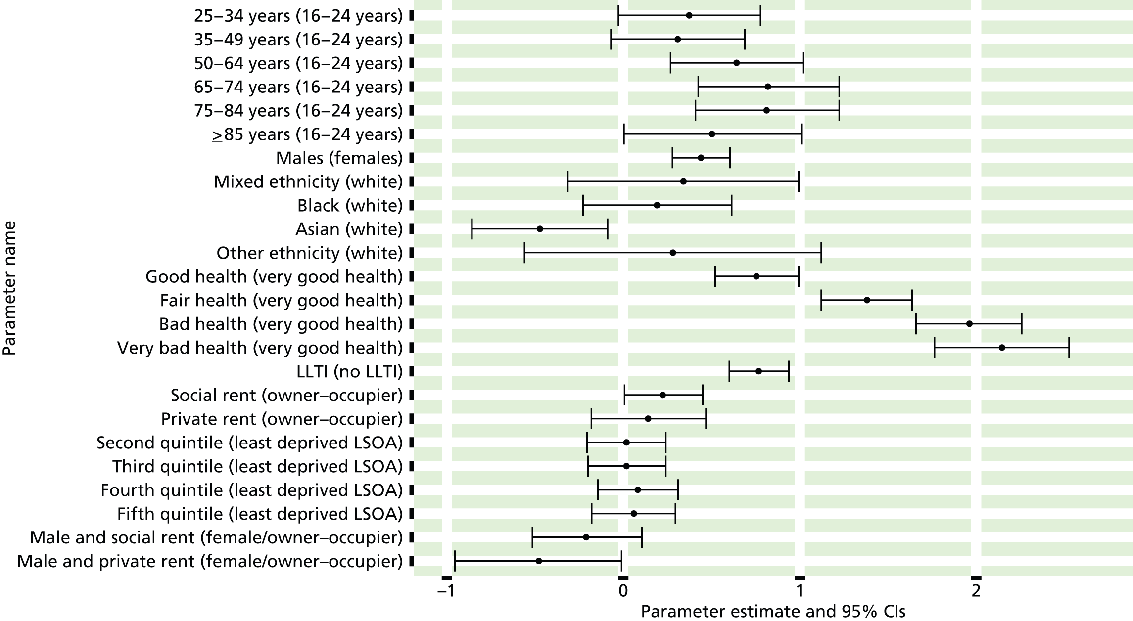
FIGURE 53.
Coronary heart disease (angina or MI) symptoms: individual estimates and their 95% CIs. (a) MSOAs; (b) LAs; (c) CCGs; and (d) regions (GORs).


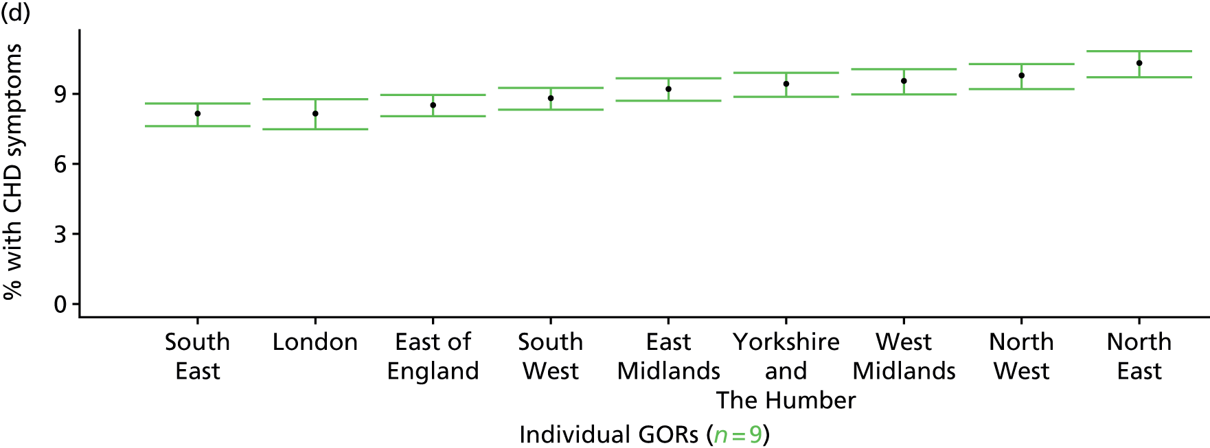
Clinical evidence of current coronary heart disease: symptoms, medication or recent doctor diagnosis (Health Survey for England, 2006 and 2011)
FIGURE 54.
Clinical evidence of current CHD: LSOA-level map. Contains Ordnance Survey data © Crown copyright and database right 2012.

Response variable definition, provenance and prediction
These estimates are based on respondents to the HSfE reporting that they had ever had symptoms of angina or MI (as described above), or who were taking prescribed drugs for CHD (see below), or who had recently (in the last 12 months) been diagnosed with angina or having had a heart attack. This is a more restricted data set largely because questions on prescribed medicines were included in the nurse-administered questionnaire, which was asked of only a subset of all respondents.
Respondents are deemed to be taking CHD drugs if they are taking any medicines classified into any of the following BNF categories specifically for ‘a heart problem’: BNF 2.4 (beta-blockers), 2.5.5.1 (ACE inhibitors), 2.6.1 (nitrates), 2.6.2 (calcium channel blockers), 2.6.3 (other antianginal drugs), 2.9 (antiplatelet drugs), 2.10.1 (drugs for management of stable angina and acute coronary symptoms) and 2.12 (lipid-regulating drugs, e.g. statins). 487
The HSfE at this time includes multiple household respondents of all ages. The analytical data set is drawn from the subset of respondents aged ≥ 16 years for whom data are available across all model response and predictor variables, namely whether or not they responded to questions on angina and MI symptoms, prescribed drug use and doctor diagnosis of angina/heart attack; whether or not they provided responses to questions on age, sex, ethnicity, general health status, LLTI and tenure; and whether or not information is available on the IMD quintile of their LSOA of residence (n = 14,896). To avoid a potential household-level effect, a single randomly selected adult is drawn from each household, resulting in an analytical data set of 9330 adults aged ≥ 16 years.
| Age band (years) | Females | Age band (years) | Males | ||||
|---|---|---|---|---|---|---|---|
| Does not have condition | Has condition | % | Does not have condition | Has condition | % | ||
| 16–24 | 405 | 14 | 3.3 | 16–24 | 236 | 6 | 2.5 |
| 25–34 | 843 | 42 | 4.7 | 25–34 | 515 | 23 | 4.3 |
| 35–49 | 1523 | 95 | 5.9 | 35–49 | 1065 | 93 | 8.0 |
| 50–64 | 1380 | 163 | 10.6 | 50–64 | 925 | 207 | 18.3 |
| 65–74 | 442 | 98 | 18.1 | 65–74 | 314 | 101 | 24.3 |
| 75–84 | 269 | 96 | 26.3 | 75–84 | 172 | 96 | 35.8 |
| ≥ 85 | 95 | 34 | 26.4 | ≥ 85 | 47 | 31 | 39.7 |
| Females | 4957 | 542 | 9.9 | Males | 3274 | 557 | 14.5 |
| Total (males and females) | 8231 | 1099 | 11.8 | ||||
Model parameters (see below) are applied to microsimulated LSOA-level census data to produce estimates of the number (and proportion) of people expected to report symptoms of CHD (angina or MI), who are taking prescribed drugs for CHD, or who have been recently diagnosed with angina and/or a heart attack in each age–sex cohort (and overall) in each of the 32,844 English LSOAs. As discussed in the report, bootstrapping is used to derive 95% CIs for these estimates. The bootstrapped LSOA-level prevalence rate estimates are aggregated into a number of higher geographies, namely for MSOAs, LAs, CCGs and regions (GORs), and are then used to calculate 95% CIs for these higher-level estimates. Proportionate attribution is used to restructure the estimates to align with 2001 MSOAs, as well as GP practice populations as defined by the 2011 NHS ADS.
Table 77 summarises how expected prevalence rates vary by age, sex and local deprivation (as measured by the 2010 IMD). There are 6569 LSOAs (with 9,226,227 adults) classified as being in the least deprived quintile; 6568 LSOAs (9,525,344 adults) in the second least deprived quintile; 6568 LSOAs (9,658,444 adults) in the third least deprived quintile; 6568 LSOAs (9,650,576 adults) in the fourth least deprived quintile; and 6568 LSOAs (9,535,167 adults) in the most deprived quintile. Note that, as a general rule, variations in prevalence rates reflect variations in the socioeconomic composition of populations in the different types of LSOA rather than variations in deprivation per se.
| Cohort | Least deprived quintile LSOAs | Second least deprived quintile LSOAs | Third least deprived quintile LSOAs | Fourth least deprived quintile LSOAs | Most deprived quintile LSOAs | All England |
|---|---|---|---|---|---|---|
| Female 16–24 | 1.9 (1.3 to 2.7) | 1.9 (1.2 to 2.8) | 2.2 (1.4 to 3.2) | 2.3 (1.5 to 3.3) | 2.9 (1.8 to 4.0) | 2.3 (1.4 to 3.2) |
| Female 25–34 | 2.8 (2.2 to 3.6) | 2.8 (2.2 to 3.7) | 3.2 (2.5 to 4.2) | 3.5 (2.7 to 4.4) | 4.7 (3.5 to 5.9) | 3.5 (2.8 to 4.4) |
| Female 35–49 | 4.1 (3.6 to 4.9) | 4.5 (3.9 to 5.3) | 5.6 (4.7 to 6.5) | 6.5 (5.5 to 7.5) | 8.9 (7.3 to 10.2) | 5.9 (5.2 to 6.6) |
| Female 50–64 | 9.6 (8.2 to 11.1) | 10.3 (8.9 to 11.8) | 12.2 (10.3 to 13.5) | 13.8 (11.9 to 15.7) | 18.5 (15.6 to 20.6) | 12.6 (11.2 to 13.8) |
| Female 65–74 | 16.4 (14.3 to 19.0) | 17.2 (15.0 to 20.3) | 19.7 (17.1 to 22.4) | 21.5 (18.6 to 24.9) | 27.2 (22.8 to 30.8) | 20.0 (17.9 to 22.4) |
| Female ≥ 75 | 28.1 (24.2 to 32.2) | 28.4 (24.8 to 32.6) | 30.9 (26.7 to 35.0) | 31.9 (27.7 to 36.4) | 36.7 (31.3 to 41.1) | 30.9 (27.5 to 34.5) |
| Females | 10.1 (8.6 to 11.7) | 10.5 (9.0 to 12.2) | 11.5 (9.7 to 13.2) | 11.5 (9.8 to 13.3) | 13.7 (11.3 to 15.6) | 11.4 (10.0 to 12.9) |
| Male 16–24 | 2.8 (1.9 to 4.1) | 2.8 (1.9 to 4.2) | 3.1 (2.0 to 4.5) | 3.1 (2.0 to 4.6) | 3.8 (2.4 to 5.3) | 3.2 (2.1 to 4.7) |
| Male 25–34 | 4.2 (3.3 to 5.4) | 4.1 (3.3 to 5.5) | 4.5 (3.6 to 5.7) | 4.6 (3.6 to 5.9) | 5.7 (4.5 to 7.2) | 4.7 (3.8 to 6.0) |
| Male 35–49 | 6.1 (5.0 to 7.2) | 6.5 (5.7 to 7.7) | 7.5 (6.5 to 8.7) | 8.2 (7.1 to 9.8) | 10.7 (9.0 to 12.4) | 7.8 (7.0 to 8.8) |
| Male 50–64 | 14.4 (12.4 to 16.3) | 15.1 (13.5 to 17.4) | 17.1 (15.3 to 19.0) | 18.3 (16.4 to 20.8) | 22.8 (20.0 to 25.2) | 17.3 (16.1 to 18.9) |
| Male 65–74 | 23.4 (20.6 to 27.2) | 24.1 (21.5 to 28.4) | 26.4 (23.5 to 30.4) | 27.7 (24.7 to 31.8) | 32.8 (28.4 to 37.4) | 26.5 (23.9 to 30.0) |
| Male ≥ 75 | 35.5 (30.9 to 41.1) | 35.7 (31.6 to 40.9) | 38.0 (33.4 to 43.0) | 38.2 (33.7 to 43.5) | 42.3 (37.3 to 46.7) | 37.6 (33.6 to 41.8) |
| Males | 13.2 (11.3 to 15.4) | 13.5 (11.8 to 15.8) | 14.1 (12.3 to 16.2) | 13.4 (11.7 to 15.7) | 15.3 (13.1 to 17.6) | 13.9 (12.4 to 15.7) |
| All | 11.6 (10.5 to 12.9) | 11.9 (10.9 to 13.4) | 12.7 (11.5 to 14.0) | 12.4 (11.1 to 13.8) | 14.5 (12.6 to 15.8) | 12.6 (12.0 to 13.4) |
| Factor (reference group) | Model coefficients | 95% CI | ||
|---|---|---|---|---|
| Estimate | Standard error | 2.5% CI | 97.50% | |
| (Intercept) | –4.92453 | 0.32457 | –5.56069 | –4.28836 |
| Age (16–24 years) | ||||
| 25–34 years | 0.49150 | 0.33791 | –0.17080 | 1.15379 |
| 35–49 years | 0.69891 | 0.31422 | 0.08303 | 1.31478 |
| 50–64 years | 1.49445 | 0.30768 | 0.89141 | 2.09749 |
| 65–74 years | 1.97509 | 0.32038 | 1.34715 | 2.60304 |
| 75–84 years | 2.49888 | 0.32677 | 1.85841 | 3.13936 |
| ≥ 85 years | 2.58399 | 0.38169 | 1.83588 | 3.33209 |
| Sex (females) | ||||
| Males | 0.69094 | 0.10226 | 0.4905 | 0.89137 |
| Ethnicity (white) | ||||
| Mixed | –0.13975 | 0.54518 | –1.20830 | 0.92879 |
| Black | 0.49575 | 0.29791 | –0.08816 | 1.07965 |
| Asian | –0.21009 | 0.29542 | –0.78911 | 0.36893 |
| Other | 0.91390 | 0.67018 | –0.39966 | 2.22746 |
| General health status (very good) | ||||
| Good health | 0.82726 | 0.12987 | 0.57272 | 1.08181 |
| Fair health | 1.58843 | 0.15226 | 1.28999 | 1.88686 |
| Bad health | 1.71657 | 0.41904 | 0.89524 | 2.53789 |
| Very bad health | –10.0834 | 178.3854 | –359.719 | 339.552 |
| LLTI (no LTTI) | ||||
| LLTI | 2.27225 | 0.54824 | 1.19769 | 3.34680 |
| Tenure (owner–occupier) | ||||
| Social rent | 0.18207 | 0.09297 | –0.00014 | 0.36429 |
| Private rent or other tenure | –0.07073 | 0.13569 | –0.33669 | 0.19522 |
| LSOA deprivation quintile (least deprived quintile) | ||||
| Second quintile | –0.04062 | 0.11234 | –0.26081 | 0.17956 |
| Third quintile | 0.02405 | 0.11098 | –0.19347 | 0.24157 |
| Fourth quintile | –0.01300 | 0.11582 | –0.24001 | 0.21400 |
| Fifth quintile ( = most deprived quintile) | 0.09913 | 0.12279 | –0.14153 | 0.33980 |
| Interaction effects | ||||
| 25–34 years and LLTI (16–24 years/no LLTI) | –0.49574 | 0.55564 | –1.58479 | 0.59331 |
| 35–49 years and LLTI (16–24 years/no LLTI) | –0.51362 | 0.51231 | –1.51776 | 0.49051 |
| 50–64 years and LLTI (16–24 years/no LLTI) | –1.01435 | 0.50152 | –1.99733 | –0.03138 |
| 65–74 years and LLTI (16–24 years/no LLTI) | –1.13331 | 0.51517 | –2.14304 | –0.12359 |
| 75–84 years and LLTI (16–24 years/no LLTI) | –1.36252 | 0.52027 | –2.38225 | –0.34279 |
| ≥ 85 years and LLTI (16–24 years/no LLTI) | –1.53061 | 0.58069 | –2.66877 | –0.39246 |
| Good health and LLTI (very good health/no LLTI) | –0.44849 | 0.28408 | –1.00529 | 0.10832 |
| Fair health and LLTI (very good health/no LLTI) | –0.83331 | 0.28652 | –1.39488 | –0.27173 |
| Bad health and LLTI (very good health/no LLTI) | –0.46839 | 0.48824 | –1.42533 | 0.48856 |
| Very bad health and LLTI (very good health/no LLTI) | 11.82463 | 178.3856 | –337.811 | 361.4604 |
| Male and LLTI (female/no LLTI) | –0.33835 | 0.14025 | –0.61325 | –0.06346 |
| Male and mixed (female/white) | –0.20454 | 0.92524 | –2.01800 | 1.60893 |
| Male and black (female/white) | –1.83615 | 0.79701 | –3.39829 | –0.27401 |
| Male and Asian (female/white) | –0.51906 | 0.46559 | –1.43162 | 0.39350 |
| Male and other (female/white) | –0.35620 | 0.92655 | –2.17223 | 1.45984 |
FIGURE 55.
Parameter plots: clinical evidence of current CHD.
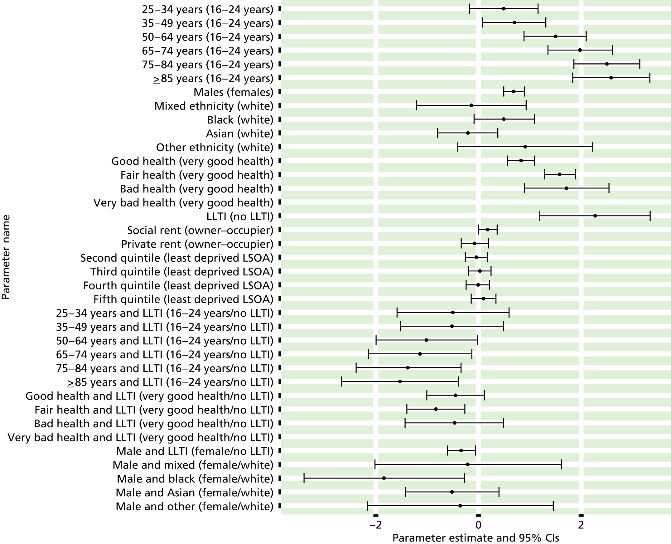
FIGURE 56.
Clinical evidence of current CHD: individual estimates and their 95% CIs. (a) MSOAs; (b) LAs; (c) CCGs; and (d) regions (GORs).


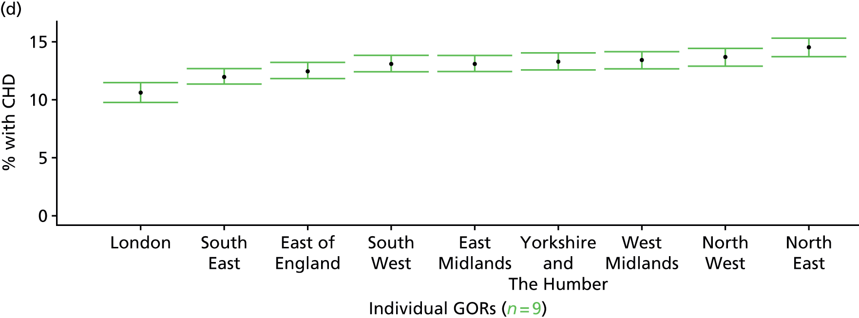
Any evidence of current coronary heart disease: symptoms, medication, recent doctor diagnosis or as self-reported long-standing illness (Health Survey for England, 2006 and 2011)
FIGURE 57.
Any evidence of current CHD: LSOA-level map. Contains Ordnance Survey data © Crown copyright and database right 2012.
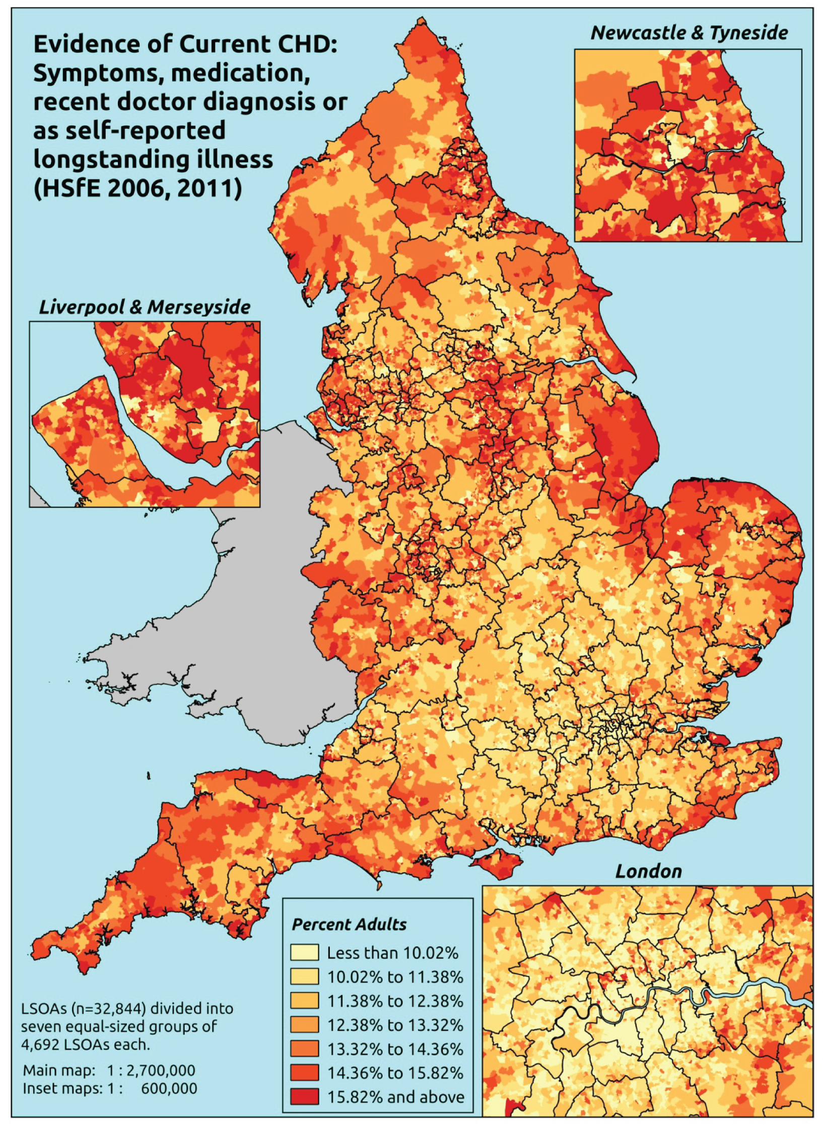
Response variable definition, provenance and prediction
These estimates are based on respondents to the HSfE reporting that they had ever had symptoms of angina or MI (as described above), or who were taking prescribed drugs for CHD (see below), or who had recently (last 12 months) been diagnosed with angina or having had a heart attack, or who self-reported angina and/or heart attack as a LSI. This is a more restricted data set largely because questions on prescribed medicines were included in the nurse-administered questionnaire, which was asked of only a subset of all respondents.
Respondents are deemed to be taking CHD drugs if they are taking any medicines classified into any of the following BNF categories specifically for ‘a heart problem’: BNF 2.4 (beta-blockers), 2.5.5.1 (ACE inhibitors), 2.6.1 (nitrates), 2.6.2 (calcium channel blockers), 2.6.3 (other antianginal drugs), 2.9 (antiplatelet drugs), 2.10.1 (drugs for management of stable angina and acute coronary symptoms) and 2.12 (lipid-regulating drugs, e.g. statins). 487
The HSfE at this time includes multiple household respondents of all ages. The analytical data set is drawn from the subset of respondents aged ≥ 16 years for whom data are available across all model response and predictor variables, namely whether or not they responded to questions on angina and MI symptoms, prescribed drug use, doctor diagnosis of angina/heart attack, and self-reported LSIs; whether or not they provided responses to questions on age, sex, ethnicity, general health status, LLTI and tenure; and whether or not information is available on the IMD quintile of their LSOA of residence (n = 14,896). To avoid a potential household-level effect, a single randomly selected adult is drawn from each household, resulting in an analytical data set of 9330 adults aged > 16 years.
| Age band (years) | Females | Age band (years) | Males | ||||
|---|---|---|---|---|---|---|---|
| Does not have condition | Has condition | % | Does not have condition | Has condition | % | ||
| 16–24 | 405 | 14 | 3.3 | 16–24 | 236 | 6 | 2.5 |
| 25–34 | 843 | 42 | 4.7 | 25–34 | 515 | 23 | 4.3 |
| 35–49 | 1522 | 96 | 5.9 | 35–49 | 1064 | 94 | 8.1 |
| 50–64 | 1380 | 163 | 10.6 | 50–64 | 924 | 208 | 18.4 |
| 65–74 | 441 | 99 | 18.3 | 65–74 | 312 | 103 | 24.8 |
| 75–84 | 267 | 98 | 26.8 | 75–84 | 166 | 102 | 38.1 |
| ≥ 85 | 94 | 35 | 27.1 | ≥ 85 | 47 | 31 | 39.7 |
| Females | 4952 | 547 | 9.9 | Males | 3264 | 567 | 14.8 |
| Total (males and females) | 8216 | 1114 | 11.9 | ||||
Model parameters (see below) are applied to microsimulated LSOA-level census data to produce estimates of the number (and proportion) of people expected to report symptoms of CHD (angina or MI), to take prescribed drugs for CHD, to have been recently diagnosed with angina and/or a heart attack, or to self-report angina and/or heart attack as a LSI in each age–sex cohort (and overall) in each of the 32,844 English LSOAs. As discussed in the report, bootstrapping is used to derive 95% CIs for these estimates. The bootstrapped LSOA-level prevalence rate estimates are aggregated into a number of higher geographies, namely for MSOAs, LAs, CCGs and regions (GORs), and are then used to calculate 95% CIs for these higher-level estimates. Proportionate attribution is used to restructure the estimates to align with 2001 MSOAs, as well as GP practice populations as defined by the 2011 NHS ADS.
Table 80 summarises how expected prevalence rates vary by age, sex and local deprivation (as measured by the 2010 IMD). There are 6569 LSOAs (with 9,226,227 adults) classified as being in the least deprived quintile; 6568 LSOAs (9,525,344 adults) in the second least deprived quintile; 6568 LSOAs (9,658,444 adults) in the third least deprived quintile; 6568 LSOAs (9,650,576 adults) in the fourth least deprived quintile; and 6568 LSOAs (9,535,167 adults) in the most deprived quintile. Note that, as a general rule, variations in prevalence rates reflect variations in the socioeconomic composition of populations in the different types of LSOA rather than variations in deprivation per se.
| Cohort | Least deprived quintile LSOAs | Second least deprived quintile LSOAs | Third least deprived quintile LSOAs | Fourth least deprived quintile LSOAs | Most deprived quintile LSOAs | All England |
|---|---|---|---|---|---|---|
| Female 16–24 | 1.9 (1.1 to 2.7) | 1.9 (1.1 to 2.8) | 2.2 (1.2 to 3.1) | 2.3 (1.2 to 3.3) | 2.9 (1.5 to 4.2) | 2.3 (1.3 to 3.2) |
| Female 25–34 | 2.7 (2.2 to 3.6) | 2.8 (2.2 to 3.6) | 3.2 (2.5 to 4.2) | 3.5 (2.7 to 4.4) | 4.6 (3.6 to 5.8) | 3.5 (2.8 to 4.4) |
| Female 35–49 | 4.1 (3.5 to 4.8) | 4.6 (3.9 to 5.4) | 5.6 (4.8 to 6.5) | 6.4 (5.5 to 7.5) | 9.0 (7.5 to 10.3) | 5.9 (5.1 to 6.8) |
| Female 50–64 | 9.4 (8.2 to 10.6) | 10.2 (9.0 to 11.6) | 12.1 (10.5 to 13.3) | 13.7 (11.9 to 15.2) | 18.5 (15.8 to 20.5) | 12.5 (11.3 to 13.4) |
| Female 65–74 | 16.3 (14.4 to 19.2) | 17.4 (15.4 to 20.2) | 19.9 (17.6 to 22.5) | 21.9 (18.9 to 25.6) | 27.7 (23.7 to 31.8) | 20.2 (18.2 to 22.6) |
| Female ≥ 75 | 28.8 (24.9 to 32.8) | 29.5 (25.6 to 34.2) | 32.0 (28.1 to 36.2) | 33.1 (28.9 to 37.3) | 38.3 (33.4 to 42.7) | 32.0 (28.4 to 35.4) |
| Females | 10.1 (8.7 to 11.7) | 10.6 (9.2 to 12.4) | 11.6 (10.0 to 13.3) | 11.6 (9.9 to 13.4) | 13.9 (11.7 to 15.9) | 11.6 (10.2 to 13.0) |
| Male 16–24 | 2.8 (1.7 to 4.0) | 2.9 (1.8 to 4.1) | 3.1 (1.9 to 4.6) | 3.1 (1.9 to 4.5) | 3.8 (2.2 to 5.5) | 3.2 (2.0 to 4.6) |
| Male 25–34 | 4.1 (3.2 to 5.6) | 4.2 (3.2 to 5.6) | 4.5 (3.6 to 6.0) | 4.6 (3.6 to 5.9) | 5.8 (4.7 to 7.5) | 4.8 (3.8 to 6.2) |
| Male 35–49 | 6.1 (4.9 to 7.1) | 6.6 (5.7 to 7.8) | 7.6 (6.7 to 8.8) | 8.2 (7.2 to 9.8) | 10.9 (9.3 to 12.7) | 7.9 (7.1 to 9.1) |
| Male 50–64 | 14.4 (12.5 to 16.6) | 15.4 (13.4 to 17.5) | 17.3 (15.2 to 19.4) | 18.4 (16.4 to 21.0) | 23.0 (20.0 to 25.3) | 17.5 (15.7 to 19.1) |
| Male 65–74 | 23.5 (20.8 to 27.5) | 24.7 (22.0 to 28.5) | 27.1 (24.5 to 30.5) | 28.3 (24.9 to 32.9) | 33.7 (29.6 to 37.6) | 27.0 (25.0 to 30.1) |
| Male ≥ 75 | 36.7 (32.9 to 42.2) | 37.5 (33.4 to 42.4) | 39.7 (35.2 to 44.3) | 40.0 (35.3 to 44.7) | 44.2 (39.5 to 48.6) | 39.2 (35.3 to 42.9) |
| Males | 13.4 (11.5 to 15.7) | 13.8 (12.1 to 16.0) | 14.4 (12.6 to 16.5) | 13.7 (11.9 to 16.0) | 15.7 (13.5 to 17.9) | 14.2 (12.7 to 16.0) |
| All | 11.7 (10.5 to 13.0) | 12.2 (11.0 to 13.5) | 13.0 (12.0 to 14.2) | 12.6 (11.5 to 13.9) | 14.8 (13.5 to 16.0) | 12.8 (12.3 to 13.5) |
| Factor (reference group) | Model coefficients | 95% CI | ||
|---|---|---|---|---|
| Estimate | Standard error | 2.5% CI | 97.50% | |
| (Intercept) | –4.95489 | 0.32479 | –5.59149 | –4.31829 |
| Age (16–24 years) | ||||
| 25–34 years | 0.49258 | 0.33796 | –0.16983 | 1.15499 |
| 35–49 years | 0.70030 | 0.31428 | 0.08432 | 1.31628 |
| 50–64 years | 1.50281 | 0.30767 | 0.89978 | 2.10585 |
| 65–74 years | 1.97679 | 0.32046 | 1.34869 | 2.60488 |
| 75–84 years | 2.53821 | 0.32635 | 1.89855 | 3.17786 |
| ≥ 85 years | 2.57509 | 0.38203 | 1.82632 | 3.32386 |
| Sex (females) | ||||
| Males | 0.70463 | 0.10216 | 0.50440 | 0.90485 |
| Ethnicity (white) | ||||
| Mixed | –0.14574 | 0.54538 | –1.21468 | 0.92320 |
| Black | 0.48636 | 0.29875 | –0.09919 | 1.07191 |
| Asian | –0.21590 | 0.29553 | –0.79515 | 0.36335 |
| Other | 0.91147 | 0.67076 | –0.40322 | 2.22616 |
| General health status (very good) | ||||
| Good health | 0.83121 | 0.12987 | 0.57667 | 1.08575 |
| Fair health | 1.59510 | 0.15215 | 1.29688 | 1.89332 |
| Bad health | 1.87210 | 0.40674 | 1.07490 | 2.66930 |
| Very bad health | 10.08105 | 178.2591 | –359.469 | 339.3068 |
| LLTI (no LTTI) | ||||
| LLTI | 2.24961 | 0.54866 | 1.17423 | 3.32498 |
| Tenure (owner–occupier) | ||||
| Social rent | 0.18471 | 0.09266 | 0.00309 | 0.36633 |
| Private rent or other tenure | –0.06563 | 0.13524 | –0.33069 | 0.19944 |
| LSOA deprivation quintile (least deprived quintile) | ||||
| Second quintile | –0.02055 | 0.11221 | –0.24049 | 0.19939 |
| Third quintile | 0.04271 | 0.11090 | –0.17466 | 0.26007 |
| Fourth quintile | 0.00416 | 0.11573 | –0.22267 | 0.23099 |
| Fifth quintile ( = most deprived quintile) | 0.12392 | 0.12263 | –0.11643 | 0.36427 |
| Interaction effects | ||||
| 25–34 years and LLTI (16–24 years/no LLTI) | –0.49693 | 0.55578 | –1.58625 | 0.59239 |
| 35–49 years and LLTI (16–24 years/no LLTI) | –0.48858 | 0.51227 | –1.49262 | 0.51546 |
| 50–64 years and LLTI (16–24 years/no LLTI) | –1.02160 | 0.50161 | –2.00477 | –0.03844 |
| 65–74 years and LLTI (16–24 years/no LLTI) | –1.09495 | 0.51514 | –2.10462 | –0.08528 |
| 75–84 years and LLTI (16–24 years/no LLTI) | –1.31511 | 0.51984 | –2.33400 | –0.29621 |
| ≥ 85 years and LLTI (16–24 years/no LLTI) | –1.47616 | 0.58059 | –2.61411 | –0.33821 |
| Good health and LLTI (very good health/no LLTI) | –0.42235 | 0.28405 | –0.97908 | 0.13439 |
| Fair health and LLTI (very good health/no LLTI) | –0.81140 | 0.28660 | –1.37314 | –0.24966 |
| Bad health and LLTI (very good health/no LLTI) | –0.60710 | 0.47787 | –1.54373 | 0.32953 |
| Very bad health and LLTI (very good health/no LLTI) | 11.85229 | 178.2593 | –337.536 | 361.2406 |
| Male and LLTI (female/no LLTI) | –0.33196 | 0.13992 | –0.60620 | –0.05772 |
| Male and mixed (female/white) | –0.22058 | 0.92577 | –2.03509 | 1.59393 |
| Male and black (female/white) | –1.84763 | 0.79787 | –3.41146 | –0.28380 |
| Male and Asian (female/white) | –0.53557 | 0.46594 | –1.44880 | 0.37767 |
| Male and other (female/white) | –0.37833 | 0.92836 | –2.19792 | 1.44125 |
FIGURE 58.
Parameter plots: any evidence of current CHD.

FIGURE 59.
Any evidence of current CHD: individual estimates and their 95% CIs. (a) MSOAs; (b) LAs; (c) CCGs; and (d) regions (GORs).


Any history of coronary heart disease: symptoms, medication, ever diagnosed or as self-reported long-standing illness (Health Survey for England, 2006 and 2011)
FIGURE 60.
Any history of CHD: LSOA-level map. Contains Ordnance Survey data © Crown copyright and database right 2012.
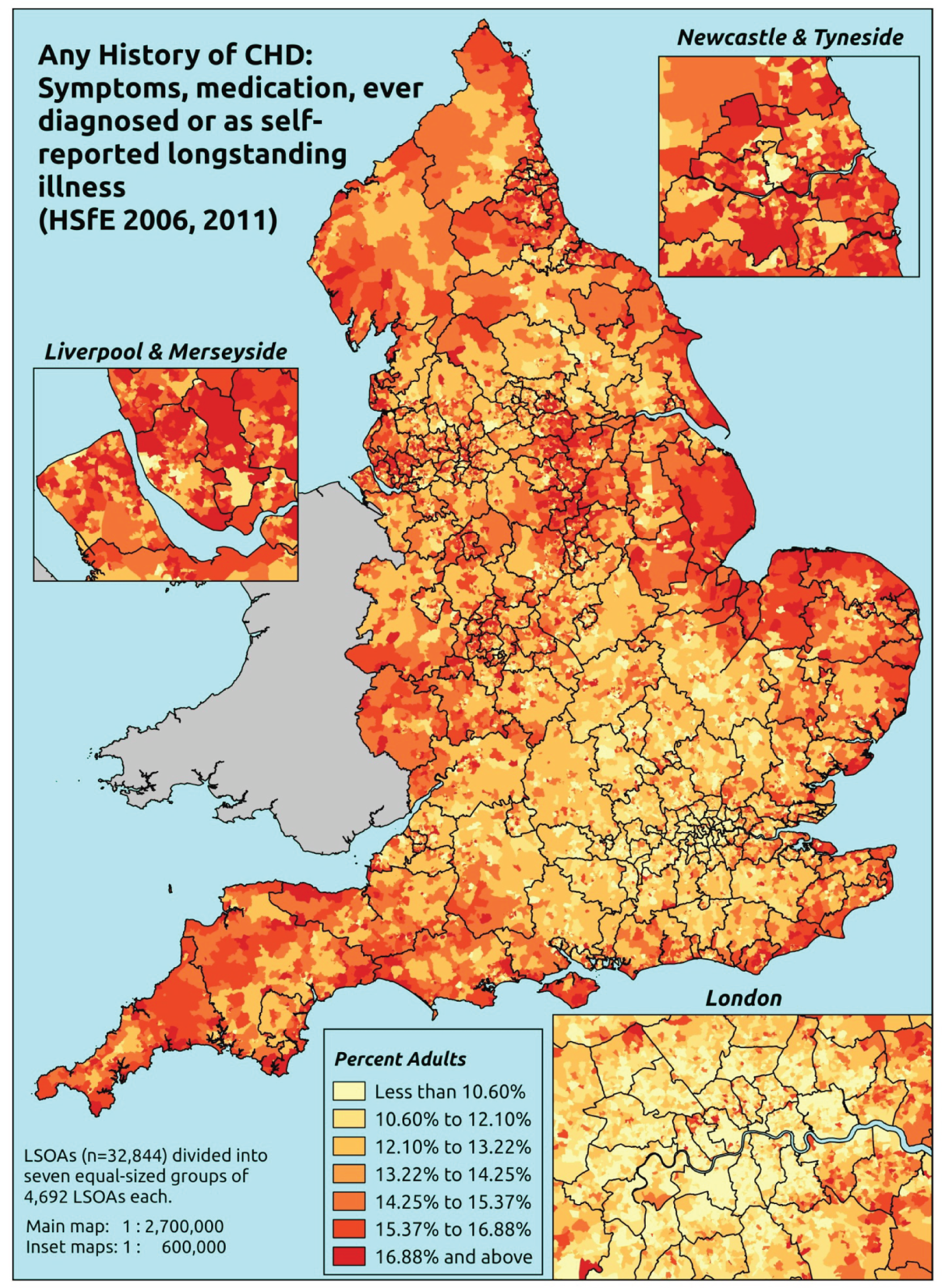
Response variable definition, provenance and prediction
These estimates are based on respondents to the HSfE reporting that they had ever had symptoms of angina or MI (as described above), or who were taking prescribed drugs for CHD (see below), or who had ever been diagnosed with angina or having had a heart attack, or who self-reported angina and/or heart attack as a LSI. This is a restricted data set largely because questions on prescribed medicines were included in the nurse-administered questionnaire, which was asked of only a subset of all respondents.
Respondents are deemed to be taking CHD drugs if they are taking any medicines classified into any of the following BNF categories specifically for ‘a heart problem’: BNF 2.4 (beta-blockers), 2.5.5.1 (ACE inhibitors), 2.6.1 (nitrates), 2.6.2 (calcium channel blockers), 2.6.3 (other antianginal drugs), 2.9 (antiplatelet drugs), 2.10.1 (drugs for management of stable angina and acute coronary symptoms) and 2.12 (lipid-regulating drugs, e.g. statins). 487
The HSfE at this time includes multiple household respondents of all ages. The analytical data set is drawn from the subset of respondents aged ≥ 16 years for whom data are available across all model response and predictor variables, namely whether or not they responded to questions on angina and MI symptoms, prescribed drug use, doctor diagnosis of angina/heart attack, and self-reported LSIs; whether or not they provided responses to questions on age, sex, ethnicity, general health status, LLTI and tenure; and whether or not information is available on the IMD quintile of their LSOA of residence (n = 14,902). To avoid a potential household-level effect, a single randomly selected adult is drawn from each household, resulting in an analytical data set of 9336 adults aged ≥ 16 years.
| Age band (years) | Females | Age band (years) | Males | ||||
|---|---|---|---|---|---|---|---|
| Does not have condition | Has condition | % | Does not have condition | Has condition | % | ||
| 16–24 | 404 | 15 | 3.6 | 16–24 | 235 | 7 | 2.9 |
| 25–34 | 843 | 42 | 4.7 | 25–34 | 515 | 23 | 4.3 |
| 35–49 | 1521 | 97 | 6.0 | 35–49 | 1061 | 98 | 8.5 |
| 50–64 | 1374 | 169 | 11.0 | 50–64 | 914 | 220 | 19.4 |
| 65–74 | 434 | 106 | 19.6 | 65–74 | 307 | 109 | 26.2 |
| 75–84 | 254 | 113 | 30.8 | 75–84 | 160 | 108 | 40.3 |
| ≥ 85 | 87 | 42 | 32.6 | ≥ 85 | 43 | 35 | 44.9 |
| Females | 4917 | 584 | 10.6 | Males | 3235 | 600 | 15.6 |
| Total (males and females) | 8152 | 1184 | 12.7 | ||||
Model parameters (see below) are applied to microsimulated LSOA-level census data to produce estimates of the number (and proportion) of people expected to report symptoms of CHD (angina or MI), to take prescribed drugs for CHD, ever to have been diagnosed with angina and/or a heart attack or to self-report angina and/or heart attack as a LSI in each age–sex cohort (and overall) in each of the 32,844 English LSOAs. As discussed in the report, bootstrapping is used to derive 95% CIs for these estimates. The bootstrapped LSOA-level prevalence rate estimates are aggregated into a number of higher geographies, namely for MSOAs, LAs, CCGs and regions (GORs), and are then used to calculate 95% CIs for these higher-level estimates. Proportionate attribution is used to restructure the estimates to align with 2001 MSOAs, as well as GP practice populations as defined by the 2011 NHS ADS.
Table 83 summarises how expected prevalence rates vary by age, sex and local deprivation (as measured by the 2010 IMD). There are 6569 LSOAs (with 9,226,227 adults) classified as being in the least deprived quintile; 6568 LSOAs (9,525,344 adults) in the second least deprived quintile; 6568 LSOAs (9,658,444 adults) in the third least deprived quintile; 6568 LSOAs (9,650,576 adults) in the fourth least deprived quintile; and 6568 LSOAs (9,535,167 adults) in the most deprived quintile. Note that, as a general rule, variations in prevalence rates reflect variations in the socioeconomic composition of populations in the different types of LSOA rather than variations in deprivation per se.
| Cohort | Least deprived quintile LSOAs | Second least deprived quintile LSOAs | Third least deprived quintile LSOAs | Fourth least deprived quintile LSOAs | Most deprived quintile LSOAs | All England |
|---|---|---|---|---|---|---|
| Female 16–24 | 2.0 (1.2 to 2.8) | 2.2 (1.3 to 3.0) | 2.4 (1.5 to 3.4) | 2.5 (1.5 to 3.5) | 3.1 (1.9 to 4.3) | 2.5 (1.5 to 3.4) |
| Female 25–34 | 2.7 (1.9 to 3.3) | 2.9 (2.2 to 3.7) | 3.2 (2.4 to 4.2) | 3.5 (2.7 to 4.4) | 4.6 (3.4 to 5.5) | 3.5 (2.7 to 4.3) |
| Female 35–49 | 4.1 (3.3 to 4.9) | 4.8 (4.0 to 5.5) | 5.7 (4.7 to 6.5) | 6.6 (5.5 to 7.7) | 9.1 (7.5 to 10.2) | 6.1 (5.2 to 6.8) |
| Female 50–64 | 9.8 (8.3 to 10.8) | 11.0 (9.4 to 12.4) | 12.6 (10.6 to 14.2) | 14.3 (12.2 to 15.9) | 19.0 (16.0 to 20.9) | 13.1 (11.6 to 14.1) |
| Female 65–74 | 17.1 (14.6 to 19.7) | 19.0 (16.3 to 22.1) | 21.0 (17.6 to 23.8) | 23.1 (20.1 to 26.4) | 28.8 (24.4 to 32.1) | 21.3 (18.6 to 23.8) |
| Female ≥ 75 | 32.3 (28.3 to 36.1) | 34.2 (30.5 to 38.9) | 36.1 (32.1 to 40.8) | 37.5 (33.5 to 41.5) | 42.4 (37.3 to 46.8) | 36.2 (33.1 to 39.8) |
| Females | 10.8 (9.2 to 12.2) | 11.8 (10.1 to 13.6) | 12.5 (10.6 to 14.3) | 12.5 (10.7 to 14.2) | 14.6 (12.2 to 16.4) | 12.4 (10.9 to 13.8) |
| Male 16–24 | 3.0 (1.8 to 4.2) | 3.2 (2.0 to 4.5) | 3.4 (2.1 to 4.8) | 3.3 (2.1 to 4.7) | 4.0 (2.6 to 5.7) | 3.4 (2.2 to 4.8) |
| Male 25–34 | 4.1 (3.1 to 5.2) | 4.3 (3.4 to 5.8) | 4.5 (3.5 to 6.0) | 4.6 (3.6 to 6.1) | 5.7 (4.5 to 7.3) | 4.7 (3.8 to 6.1) |
| Male 35–49 | 6.1 (5.2 to 7.1) | 6.8 (5.9 to 8.0) | 7.7 (6.6 to 8.9) | 8.4 (7.2 to 9.9) | 11.0 (9.2 to 12.5) | 8.0 (7.1 to 9.1) |
| Male 50–64 | 14.9 (13.1 to 16.7) | 16.5 (14.6 to 18.8) | 18.1 (15.9 to 20.5) | 19.3 (17.0 to 22.1) | 23.7 (20.7 to 26.1) | 18.3 (16.7 to 20.0) |
| Male 65–74 | 24.7 (21.7 to 28.4) | 26.7 (23.9 to 30.7) | 28.5 (25.6 to 32.3) | 29.9 (27.3 to 34.6) | 34.8 (30.9 to 39.6) | 28.5 (26.3 to 31.8) |
| Male ≥ 75 | 40.5 (37.0 to 45.2) | 42.5 (38.6 to 47.9) | 44.0 (40.8 to 49.3) | 44.4 (40.1 to 50.0) | 48.3 (43.0 to 53.3) | 43.6 (40.7 to 48.1) |
| Males | 14.1 (12.3 to 16.1) | 15.0 (13.3 to 17.4) | 15.2 (13.5 to 17.5) | 14.5 (12.7 to 16.9) | 16.3 (14.0 to 18.6) | 15.0 (13.6 to 16.9) |
| All | 12.4 (11.2 to 13.6) | 13.4 (12.2 to 14.9) | 13.8 (12.5 to 15.2) | 13.4 (12.2 to 14.9) | 15.4 (14.0 to 16.7) | 13.7 (13.2 to 14.4) |
| Factor (reference group) | Model coefficients | 95% CI | ||
|---|---|---|---|---|
| Estimate | Standard error | 2.5% CI | 97.50% | |
| (Intercept) | –4.81247 | 0.30464 | –5.40955 | –4.21538 |
| Age (16–24 years) | ||||
| 25–34 years | 0.33176 | 0.31980 | –0.29504 | 0.95856 |
| 35–49 years | 0.55836 | 0.29445 | –0.01876 | 1.13548 |
| 50–64 years | 1.41872 | 0.28691 | 0.85638 | 1.98106 |
| 65–74 years | 1.92250 | 0.29962 | 1.33524 | 2.50976 |
| 75–84 years | 2.49131 | 0.30602 | 1.89151 | 3.09111 |
| ≥ 85 years | 2.64601 | 0.36032 | 1.93978 | 3.35224 |
| Sex (females) | ||||
| Males | 0.68817 | 0.09975 | 0.49266 | 0.88367 |
| Ethnicity (white) | ||||
| Mixed | –0.18120 | 0.54516 | –1.24971 | 0.88732 |
| Black | 0.44693 | 0.29986 | –0.14079 | 1.03466 |
| Asian | –0.03476 | 0.27323 | –0.57030 | 0.50078 |
| Other | 0.87699 | 0.67054 | –0.43727 | 2.19125 |
| General health status (very good) | ||||
| Good health | 0.84024 | 0.12664 | 0.59203 | 1.08845 |
| Fair health | 1.61050 | 0.14867 | 1.31910 | 1.90189 |
| Bad health | 1.78240 | 0.40847 | 0.98180 | 2.58300 |
| Very bad health | –10.1535 | 178.462 | –359.939 | 339.6321 |
| LLTI (no LTTI) | ||||
| LLTI | 2.05713 | 0.53598 | 1.00661 | 3.10766 |
| Tenure (owner–occupier) | ||||
| Social rent | 0.17008 | 0.09165 | –0.00955 | 0.34971 |
| Private rent or other tenure | –0.04505 | 0.13242 | –0.30460 | 0.21450 |
| LSOA deprivation quintile (least deprived quintile) | ||||
| Second quintile | 0.02449 | 0.10979 | –0.19070 | 0.23967 |
| Third quintile | 0.05303 | 0.10913 | –0.16086 | 0.26692 |
| Fourth quintile | 0.01869 | 0.11386 | –0.20447 | 0.24186 |
| Fifth quintile ( = most deprived quintile) | 0.12085 | 0.12110 | –0.11651 | 0.35820 |
| Interaction effects | ||||
| 25–34 years and LLTI (16–24 years/no LLTI) | –0.33521 | 0.54500 | –1.40342 | 0.73299 |
| 35–49 years and LLTI (16–24 years/no LLTI) | –0.31139 | 0.50018 | –1.29175 | 0.66896 |
| 50–64 years and LLTI (16–24 years/no LLTI) | –0.90205 | 0.48916 | –1.86079 | 0.05669 |
| 65–74 years and LLTI (16–24 years/no LLTI) | –0.97888 | 0.50231 | –1.96341 | 0.00564 |
| 75–84 years and LLTI (16–24 years/no LLTI) | –1.08844 | 0.50704 | –2.08225 | –0.09464 |
| ≥ 85 years and LLTI (16–24 years/no LLTI) | –1.26860 | 0.56439 | –2.37481 | –0.16239 |
| Good health and LLTI (very good health/no LLTI) | –0.40604 | 0.27922 | –0.95331 | 0.14123 |
| Fair health and LLTI (very good health/no LLTI) | –0.80597 | 0.28183 | –1.35837 | –0.25358 |
| Bad health and LLTI (very good health/no LLTI) | –0.44655 | 0.47763 | –1.38271 | 0.48961 |
| Very bad health and LLTI (very good health/no LLTI) | 11.9581 | 178.4623 | –337.828 | 361.7441 |
| Male and mixed (female/white) | –0.20582 | 0.92530 | –2.01942 | 1.60777 |
| Male and black (female/white) | –1.85692 | 0.79963 | –3.42420 | –0.28965 |
| Male and Asian (female/white) | –0.75543 | 0.45228 | –1.64189 | 0.13104 |
| Male and other (female/white) | –0.40665 | 0.93380 | –2.23689 | 1.42359 |
| Male and LLTI (female/no LLTI) | –0.30108 | 0.13758 | –0.57074 | –0.03143 |
FIGURE 61.
Parameter plots: any history of CHD.
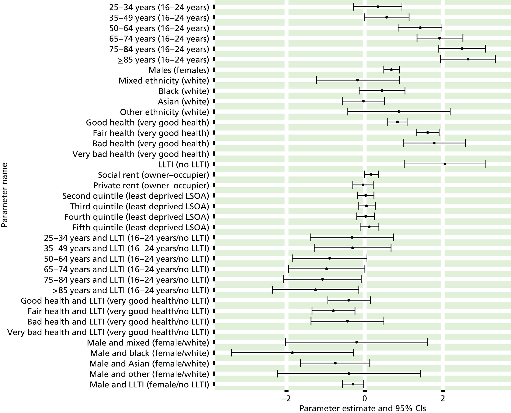
FIGURE 62.
Any history of CHD: individual estimates and their 95% CIs. (a) MSOAs; (b) LAs; (c) CCGs; and (d) regions (GORs).


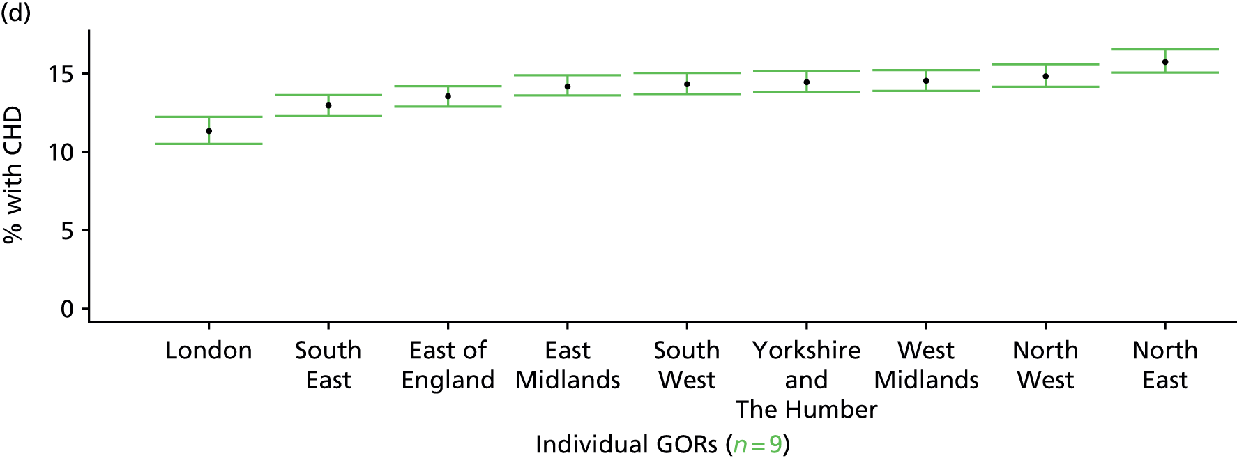
Ever been diagnosed with coronary heart disease (Health Survey for England, 2006 and 2011)
FIGURE 63.
Ever diagnosed with CHD: LSOA-level map. Contains Ordnance Survey data © Crown copyright and database right 2012.
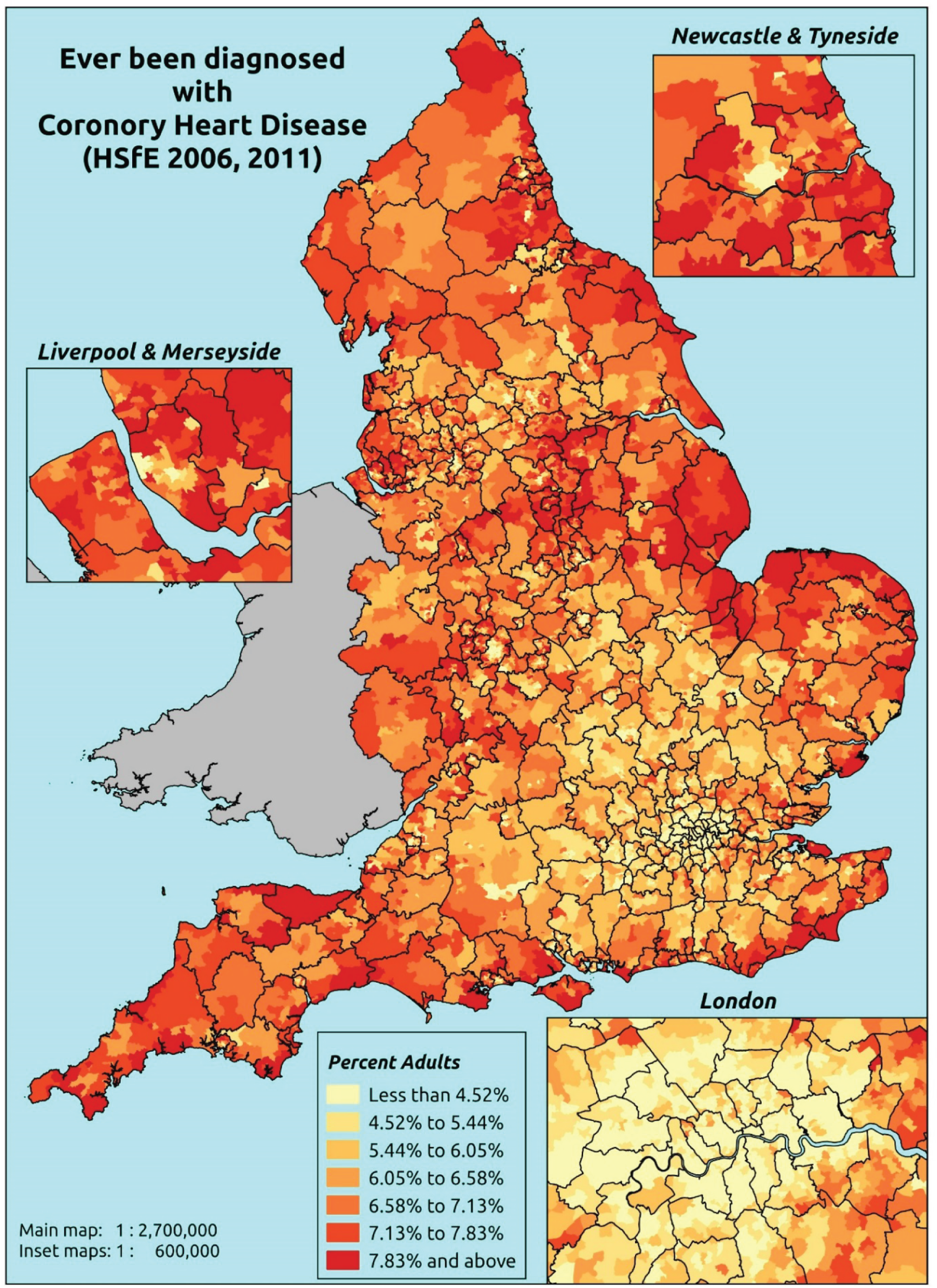
Response variable definition, provenance and prediction
These estimates are based on respondents to the HSfE reporting that they had ever been diagnosed with angina or having had a heart attack.
The HSfE at this time includes multiple household respondents of all ages. The analytical data set is drawn from the subset of respondents aged ≥ 16 years for whom data are available across all model response and predictor variables, namely whether or not they responded to questions on doctor diagnosis of angina/heart attack; whether or not they provided responses to questions on age, sex, ethnicity, general health status, LLTI and tenure; and whether or not information is available on the IMD quintile of their LSOA of residence (n = 20,952). To avoid a potential household-level effect, a single randomly selected adult is drawn from each household, resulting in an analytical data set of 12,822 adults aged ≥ 16 years.
| Age band (years) | Females | Age band (years) | Males | ||||
|---|---|---|---|---|---|---|---|
| Does not have condition | Has condition | % | Does not have condition | Has condition | % | ||
| 16–24 | 569 | 1 | 0.2 | 16–24 | 428 | 1 | 0.2 |
| 25–34 | 1213 | 5 | 0.4 | 25–34 | 811 | 2 | 0.2 |
| 35–49 | 2187 | 12 | 0.5 | 35–49 | 1517 | 22 | 1.4 |
| 50–64 | 1916 | 65 | 3.3 | 50–64 | 1361 | 129 | 8.7 |
| 65–74 | 669 | 72 | 9.7 | 65–74 | 456 | 102 | 18.3 |
| 75–84 | 474 | 100 | 17.4 | 75–84 | 275 | 96 | 25.9 |
| ≥ 85 | 167 | 49 | 22.7 | ≥ 85 | 89 | 34 | 27.6 |
| Females | 7195 | 304 | 4.1 | Males | 4937 | 386 | 7.3 |
| Total (males and females) | 12,132 | 690 | 5.4 | ||||
Model parameters (see below) are applied to microsimulated LSOA-level census data to produce estimates of the number (and proportion) of people expected ever to have been diagnosed with angina and/or a heart attack in each age–sex cohort (and overall) in each of the 32,844 English LSOAs. As discussed in the report, bootstrapping is used to derive 95% CIs for these estimates. The bootstrapped LSOA-level prevalence rate estimates are aggregated into a number of higher geographies, namely for MSOAs, LAs, CCGs and regions (GORs), and are then used to calculate 95% CIs for these higher-level estimates. Proportionate attribution is used to restructure the estimates to align with 2001 MSOAs, as well as GP practice populations as defined by the 2011 NHS ADS.
Table 86 summarises how expected prevalence rates vary by age, sex and local deprivation (as measured by the 2010 IMD). There are 6569 LSOAs (with 9,226,227 adults) classified as being in the least deprived quintile; 6568 LSOAs (9,525,344 adults) in the second least deprived quintile; 6568 LSOAs (9,658,444 adults) in the third least deprived quintile; 6568 LSOAs (9,650,576 adults) in the fourth least deprived quintile; and 6568 LSOAs (9,535,167 adults) in the most deprived quintile. Note that, as a general rule, variations in prevalence rates reflect variations in the socioeconomic composition of populations in the different types of LSOA rather than variations in deprivation per se.
| Cohort | Least deprived quintile LSOAs | Second least deprived quintile LSOAs | Third least deprived quintile LSOAs | Fourth least deprived quintile LSOAs | Most deprived quintile LSOAs | All England |
|---|---|---|---|---|---|---|
| Female 16–24 | 0.1 (0.0 to 0.2) | 0.1 (0.0 to 0.2) | 0.1 (0.0 to 0.2) | 0.1 (0.0 to 0.3) | 0.1 (0.0 to 0.3) | 0.1 (0.0 to 0.3) |
| Female 25–34 | 0.2 (0.1 to 0.3) | 0.2 (0.1 to 0.3) | 0.2 (0.1 to 0.3) | 0.2 (0.1 to 0.3) | 0.2 (0.1 to 0.4) | 0.2 (0.1 to 0.3) |
| Female 35–49 | 0.4 (0.3 to 0.6) | 0.5 (0.3 to 0.6) | 0.5 (0.3 to 0.7) | 0.6 (0.4 to 0.8) | 0.8 (0.5 to 1.1) | 0.6 (0.4 to 0.7) |
| Female 50–64 | 3.2 (2.5 to 3.9) | 3.3 (2.7 to 4.2) | 3.6 (2.8 to 4.4) | 4.5 (3.7 to 5.5) | 5.8 (4.7 to 7.3) | 4.0 (3.4 to 4.8) |
| Female 65–74 | 8.9 (7.2 to 11.2) | 9.3 (7.7 to 11.4) | 9.8 (7.9 to 11.7) | 11.9 (10.0 to 14.5) | 14.7 (12.3 to 17.6) | 10.7 (9.4 to 12.5) |
| Female ≥ 75 | 19.2 (16.1 to 22.9) | 19.4 (16.2 to 22.5) | 19.7 (16.1 to 22.8) | 22.2 (19.2 to 26.2) | 25.1 (21.1 to 29.4) | 20.9 (18.5 to 23.5) |
| Females | 4.8 (3.9 to 5.8) | 4.9 (4.0 to 5.9) | 4.8 (3.9 to 5.7) | 5.0 (4.2 to 6.1) | 5.4 (4.4 to 6.6) | 5.0 (4.3 to 5.8) |
| Male 16–24 | 0.2 (0.0 to 0.5) | 0.2 (0.0 to 0.4) | 0.2 (0.0 to 0.4) | 0.2 (0.0 to 0.5) | 0.2 (0.0 to 0.5) | 0.2 (0.0 to 0.5) |
| Male 25–34 | 0.3 (0.2 to 0.6) | 0.3 (0.2 to 0.6) | 0.3 (0.1 to 0.6) | 0.4 (0.2 to 0.7) | 0.4 (0.2 to 0.9) | 0.4 (0.2 to 0.7) |
| Male 35–49 | 0.8 (0.6 to 1.2) | 0.9 (0.6 to 1.3) | 1.0 (0.6 to 1.3) | 1.2 (0.8 to 1.7) | 1.6 (1.0 to 2.0) | 1.1 (0.7 to 1.5) |
| Male 50–64 | 6.0 (5.0 to 7.3) | 6.5 (5.4 to 7.9) | 6.9 (5.7 to 8.2) | 8.5 (7.2 to 10.1) | 11.0 (9.2 to 13.0) | 7.6 (6.8 to 8.6) |
| Male 65–74 | 16.1 (13.0 to 19.2) | 16.8 (13.9 to 20.2) | 17.6 (14.9 to 20.7) | 20.8 (17.8 to 24.7) | 25.0 (21.4 to 29.1) | 18.8 (16.7 to 21.4) |
| Male ≥ 75 | 29.6 (26.1 to 34.2) | 29.9 (26.0 to 34.2) | 30.3 (26.7 to 33.9) | 33.6 (29.6 to 37.8) | 37.5 (32.8 to 41.6) | 31.7 (28.8 to 34.9) |
| Males | 7.3 (6.1 to 8.7) | 7.4 (6.2 to 8.9) | 7.1 (6.0 to 8.3) | 7.2 (6.1 to 8.5) | 7.8 (6.6 to 9.2) | 7.4 (6.5 to 8.4) |
| All | 6.0 (5.2 to 7.0) | 6.1 (5.3 to 7.0) | 5.9 (5.2 to 6.8) | 6.1 (5.4 to 7.0) | 6.6 (5.7 to 7.5) | 6.1 (5.8 to 6.6) |
| Factor (reference group) | Model coefficients | 95% CI | ||
|---|---|---|---|---|
| Estimate | Standard error | 2.5% CI | 97.50% | |
| (Intercept) | –7.64770 | 0.73784 | –9.09387 | –6.20153 |
| Age (16–24 years) | ||||
| 25–34 years | 0.49267 | 0.80416 | –1.08348 | 2.06882 |
| 35–49 years | 1.26850 | 0.73395 | –0.17005 | 2.70705 |
| 50–64 years | 2.92336 | 0.71751 | 1.51703 | 4.32969 |
| 65–74 years | 3.83791 | 0.71935 | 2.42798 | 5.24783 |
| 75–84 years | 4.26889 | 0.71974 | 2.85819 | 5.67958 |
| ≥ 85 years | 4.45869 | 0.72742 | 3.03295 | 5.88442 |
| Sex (females) | ||||
| Males | 0.71734 | 0.08910 | 0.54270 | 0.89199 |
| Ethnicity (white) | ||||
| Mixed | –13.8491 | 602.4447 | –1194.64 | 1166.943 |
| Black | –14.0686 | 334.0905 | –668.886 | 640.7489 |
| Asian | 0.73582 | 0.29273 | 0.16208 | 1.30957 |
| Other | –13.9996 | 779.1782 | –1541.19 | 1513.19 |
| General health status (very good) | ||||
| Good health | 0.94033 | 0.18918 | 0.56954 | 1.31111 |
| Fair health | 1.61822 | 0.19548 | 1.23508 | 2.00137 |
| Bad health | 2.24823 | 0.21874 | 1.81949 | 2.67696 |
| Very bad health | 2.36815 | 0.25683 | 1.86476 | 2.87153 |
| LLTI (no LTTI) | ||||
| LLTI | 0.54187 | 0.12488 | 0.29711 | 0.78664 |
| Tenure (owner–occupier) | ||||
| Social rent | –0.07752 | 0.20538 | –0.48006 | 0.32503 |
| Private rent or other tenure | –0.07752 | 0.20538 | –0.48006 | 0.32503 |
| LSOA deprivation quintile (least deprived quintile) | ||||
| Second quintile | –0.06638 | 0.14164 | –0.34399 | 0.21123 |
| Third quintile | –0.08457 | 0.14324 | –0.36531 | 0.19617 |
| Fourth quintile | 0.00441 | 0.14786 | –0.28539 | 0.29421 |
| Fifth quintile ( = most deprived quintile) | 0.08117 | 0.15542 | –0.22345 | 0.38578 |
| Interaction effects | ||||
| LLTI and social rent (no LLTI/owner–occupier) | 0.18634 | 0.23446 | –0.27320 | 0.64588 |
| LLTI and private rent (no LLTI/owner–occupier) | –0.72387 | 0.36262 | –1.43459 | –0.01314 |
| Mixed and LLTI (white/no LLTI) | 13.87347 | 602.4453 | –1166.92 | 1194.666 |
| Black and LLTI (white/no LLTI) | 13.10224 | 334.0911 | –641.716 | 667.9209 |
| Asian and LLTI (white/no LLTI) | –0.93577 | 0.49708 | –1.91006 | 0.03851 |
| Other and LLTI (white/no LLTI) | 13.68275 | 779.1787 | –1513.51 | 1540.873 |
FIGURE 64.
Parameter plots: ever diagnosed with CHD.
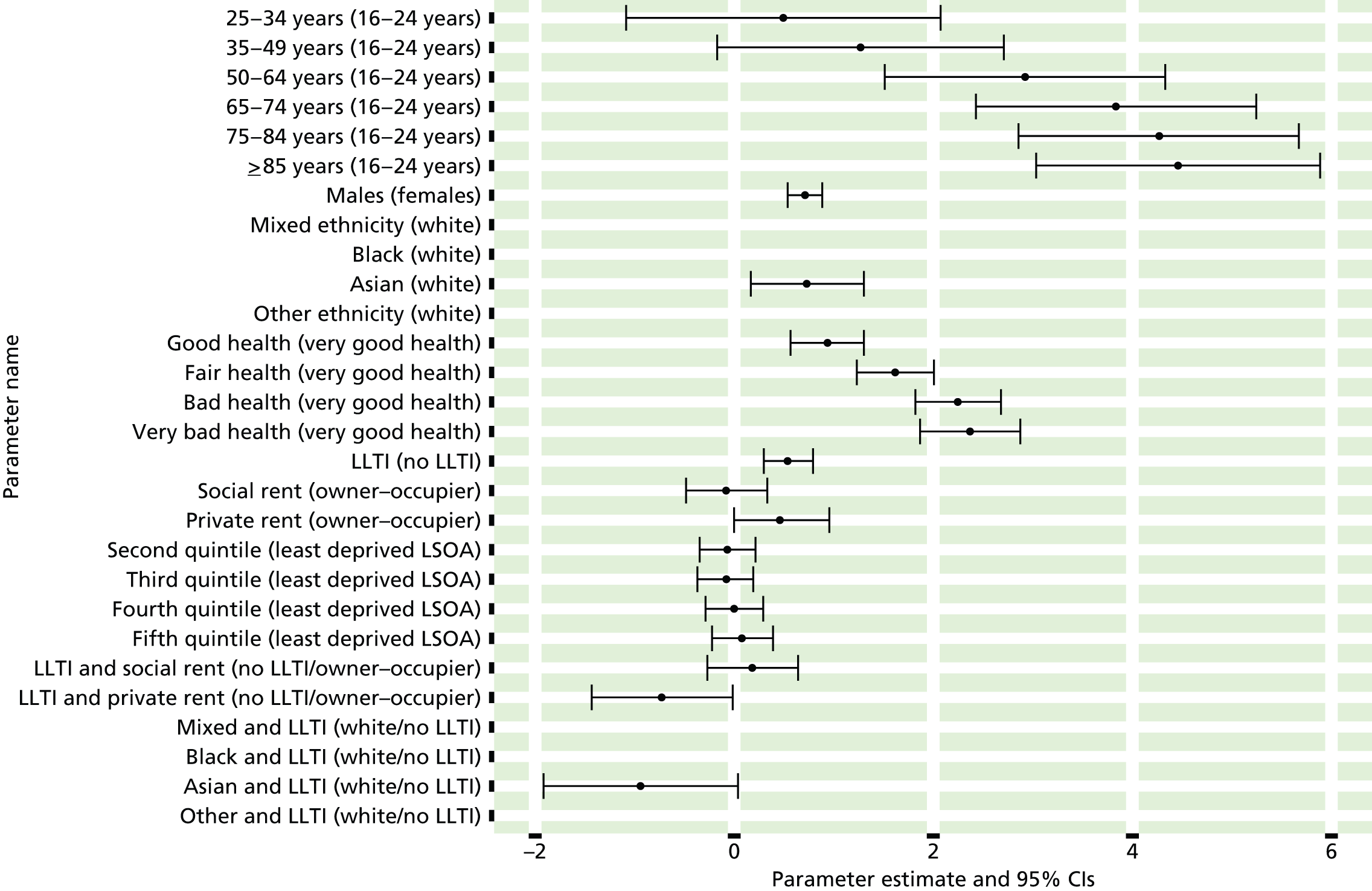
FIGURE 65.
Ever diagnosed with CHD: individual estimates and their 95% CIs. (a) MSOAs; (b) LAs; (c) CCGs; and (d) regions (GORs).


Ever been diagnosed with cardiovascular disease (Health Survey for England, 2006a and 2011)
FIGURE 66.
Ever diagnosed with CVD: LSOA-level map. Contains Ordnance Survey data © Crown copyright and database right 2012.

Response variable definition, provenance and prediction
These estimates are based on respondents to the HSfE reporting that they had ever been diagnosed with CVD. Specifically, that the respondent had been ‘told by a doctor’ that they had angina, or had had a heart attack, or had a heart murmur, or an abnormal heart rhythm, or another heart problem, or had had a stroke.
The HSfE at this time includes multiple household respondents of all ages. The analytical data set is drawn from the subset of respondents aged ≥ 16 years for whom data are available across all model response and predictor variables, namely whether or not they responded to questions on doctor diagnosis of CVD conditions; whether or not they provided responses to questions on age, sex, ethnicity, general health status, LLTI and tenure; and whether or not information is available on the IMD quintile of their LSOA of residence (n = 20,925). To avoid a potential household-level effect, a single randomly selected adult is drawn from each household, resulting in an analytical data set of 12,803 adults aged ≥ 16 years.
| Age band (years) | Females | Age band (years) | Males | ||||
|---|---|---|---|---|---|---|---|
| Does not have condition | Has condition | % | Does not have condition | Has condition | % | ||
| 16–24 | 540 | 29 | 5.1 | 16–24 | 413 | 16 | 3.7 |
| 25–34 | 1135 | 83 | 6.8 | 25–34 | 766 | 46 | 5.7 |
| 35–49 | 2015 | 179 | 8.2 | 35–49 | 1419 | 115 | 7.5 |
| 50–64 | 1681 | 298 | 15.1 | 50–64 | 1227 | 259 | 17.4 |
| 65–74 | 567 | 173 | 23.4 | 65–74 | 361 | 198 | 35.4 |
| 75–84 | 362 | 213 | 37.0 | 75–84 | 209 | 162 | 43.7 |
| ≥ 85 | 130 | 85 | 39.5 | ≥ 85 | 65 | 57 | 46.7 |
| Females | 6430 | 1060 | 14.2 | Males | 4460 | 853 | 16.1 |
| Total (males and females) | 10,890 | 1913 | 14.9 | ||||
Model parameters (see below) are applied to microsimulated LSOA-level census data to produce estimates of the number (and proportion) of people expected ever to have been diagnosed with CVD (specifically angina, heart attack, heart murmur, abnormal heart rhythm, another heart problem, stroke) in each age–sex cohort (and overall) in each of the 32,844 English LSOAs. As discussed in the report, bootstrapping is used to derive 95% CIs for these estimates. The bootstrapped LSOA-level prevalence rate estimates are aggregated into a number of higher geographies, namely for MSOAs, LAs, CCGs and regions (GORs), and are then used to calculate 95% CIs for these higher-level estimates. Proportionate attribution is used to restructure the estimates to align with 2001 MSOAs, as well as GP practice populations as defined by the 2011 NHS ADS.
Table 89 summarises how expected prevalence rates vary by age, sex and local deprivation (as measured by the 2010 IMD). There are 6569 LSOAs (with 9,226,227 adults) classified as being in the least deprived quintile; 6568 LSOAs (9,525,344 adults) in the second least deprived quintile; 6568 LSOAs (9,658,444 adults) in the third least deprived quintile; 6568 LSOAs (9,650,576 adults) in the fourth least deprived quintile; and 6568 LSOAs (9,535,167 adults) in the most deprived quintile. Note that, as a general rule, variations in prevalence rates reflect variations in the socioeconomic composition of populations in the different types of LSOA rather than variations in deprivation per se.
| Cohort | Least deprived quintile LSOAs | Second least deprived quintile LSOAs | Third least deprived quintile LSOAs | Fourth least deprived quintile LSOAs | Most deprived quintile LSOAs | All England |
|---|---|---|---|---|---|---|
| Female 16–24 | 3.9 (2.6 to 5.4) | 3.9 (2.6 to 5.3) | 4.1 (2.7 to 5.6) | 4.2 (2.8 to 5.8) | 4.3 (2.9 to 5.7) | 4.1 (2.7 to 5.6) |
| Female 25–34 | 5.3 (4.1 to 6.7) | 5.4 (4.3 to 6.7) | 5.7 (4.6 to 7.2) | 5.9 (4.9 to 7.4) | 6.2 (5.1 to 7.6) | 5.8 (4.8 to 7.1) |
| Female 35–49 | 7.0 (6.0 to 8.1) | 7.4 (6.3 to 8.6) | 8.1 (6.8 to 9.4) | 8.8 (7.6 to 10.3) | 9.5 (8.2 to 11.2) | 8.2 (7.3 to 9.3) |
| Female 50–64 | 13.3 (11.6 to 15.2) | 14.0 (12.7 to 15.6) | 15.4 (13.8 to 17.3) | 16.9 (15.3 to 19.3) | 18.9 (16.4 to 21.4) | 15.5 (14.3 to 17.0) |
| Female 65–74 | 21.9 (18.9 to 24.9) | 22.9 (19.9 to 26.2) | 24.7 (21.6 to 27.8) | 26.8 (24.0 to 30.1) | 29.1 (25.5 to 32.9) | 24.8 (22.2 to 27.2) |
| Female ≥ 75 | 39.6 (36.0 to 42.9) | 40.5 (36.9 to 43.9) | 42.4 (38.9 to 46.3) | 44.2 (40.6 to 48.1) | 45.2 (41.5 to 49.8) | 42.2 (39.2 to 45.2) |
| Females | 14.6 (12.7 to 16.5) | 15.1 (13.3 to 17.0) | 15.6 (13.7 to 17.6) | 15.4 (13.7 to 17.6) | 15.5 (13.5 to 17.7) | 15.2 (13.7 to 16.9) |
| Male 16–24 | 2.9 (1.4 to 4.2) | 2.9 (1.4 to 4.4) | 3.1 (1.6 to 4.4) | 3.1 (1.7 to 4.6) | 3.2 (1.6 to 4.6) | 3.0 (1.6 to 4.4) |
| Male 25–34 | 4.3 (3.1 to 5.7) | 4.3 (3.1 to 5.8) | 4.6 (3.3 to 6.1) | 4.8 (3.5 to 6.3) | 5.1 (3.8 to 6.6) | 4.7 (3.5 to 5.9) |
| Male 35–49 | 5.6 (4.4 to 6.5) | 5.9 (4.7 to 7.0) | 6.6 (5.3 to 7.6) | 7.3 (6.0 to 8.7) | 8.3 (6.9 to 9.7) | 6.7 (5.6 to 7.7) |
| Male 50–64 | 14.5 (12.7 to 16.2) | 15.5 (13.7 to 17.4) | 17.3 (15.1 to 19.4) | 19.3 (17.5 to 21.7) | 22.0 (19.5 to 25.0) | 17.5 (15.8 to 19.2) |
| Male 65–74 | 32.5 (28.0 to 35.8) | 34.0 (29.3 to 37.5) | 36.7 (31.8 to 40.6) | 39.6 (35.4 to 44.1) | 43.0 (37.8 to 47.4) | 36.7 (32.9 to 40.2) |
| Male ≥ 75 | 45.9 (41.6 to 50.3) | 47.1 (42.6 to 51.2) | 49.3 (45.1 to 54.0) | 51.3 (47.0 to 56.2) | 53.0 (48.3 to 57.0) | 49.0 (45.1 to 52.6) |
| Males | 15.5 (13.3 to 17.5) | 16.0 (13.8 to 18.0) | 16.3 (14.0 to 18.4) | 15.7 (13.8 to 18.0) | 16.1 (13.8 to 18.3) | 15.9 (14.0 to 17.7) |
| All | 15.0 (13.8 to 16.1) | 15.5 (14.4 to 16.6) | 15.9 (14.7 to 17.1) | 15.6 (14.5 to 16.9) | 15.8 (14.6 to 16.8) | 15.6 (15.0 to 16.1) |
| Factor (reference group) | Model coefficients | 95% CI | ||
|---|---|---|---|---|
| Estimate | Standard error | 2.5% CI | 97.50% | |
| (Intercept) | –3.56047 | 0.22354 | –3.99861 | –3.12234 |
| Age (16–24 years) | ||||
| 25–34 years | 0.33101 | 0.23137 | –0.12247 | 0.78448 |
| 35–49 years | 0.46484 | 0.21578 | 0.04191 | 0.88778 |
| 50–64 years | 0.93751 | 0.21255 | 0.52091 | 1.35412 |
| 65–74 years | 1.40494 | 0.22217 | 0.96947 | 1.84040 |
| 75–84 years | 1.92357 | 0.22292 | 1.48665 | 2.36049 |
| ≥ 85 years | 2.02663 | 0.25035 | 1.53594 | 2.51733 |
| Sex (females) | ||||
| Males | –0.23803 | 0.35109 | –0.92616 | 0.45010 |
| Ethnicity (white) | ||||
| Mixed | 0.60826 | 0.34753 | –0.07290 | 1.28942 |
| Black | –0.54887 | 0.27694 | –1.09167 | –0.00606 |
| Asian | –0.94766 | 0.26724 | –1.47145 | –0.42387 |
| Other | –0.78668 | 0.77192 | –2.29964 | 0.72627 |
| General health status (very good) | ||||
| Good health | 0.61274 | 0.10625 | 0.40448 | 0.82099 |
| Fair health | 0.86985 | 0.12114 | 0.63241 | 1.10730 |
| Bad health | 1.32434 | 0.15767 | 1.01530 | 1.63338 |
| Very bad health | 1.49338 | 0.22072 | 1.06077 | 1.92600 |
| LLTI (no LTTI) | ||||
| LLTI | 0.54616 | 0.06824 | 0.41240 | 0.67992 |
| Tenure (owner–occupier) | ||||
| Social rent | –0.10644 | 0.07692 | –0.25720 | 0.04432 |
| Private rent or other tenure | 0.14435 | 0.09778 | –0.04729 | 0.33600 |
| LSOA deprivation quintile (least deprived quintile) | ||||
| Second quintile | –0.01650 | 0.08740 | –0.18781 | 0.15481 |
| Third quintile | 0.03072 | 0.08763 | –0.14102 | 0.20247 |
| Fourth quintile | 0.06026 | 0.09056 | –0.11725 | 0.23777 |
| Fifth quintile ( = most deprived quintile) | 0.07094 | 0.09717 | –0.11950 | 0.26139 |
| Interaction effects | ||||
| 25–34 years and male (16–24 years/female) | 0.05380 | 0.38493 | –0.70065 | 0.80825 |
| 35–49 years and male (16–24 years/female) | 0.05233 | 0.35584 | –0.64513 | 0.74978 |
| 50–64 years and male (16–24 years/female) | 0.37142 | 0.34654 | –0.30781 | 1.05064 |
| 65–74 years and male (16–24 years/female) | 0.78792 | 0.35761 | 0.08701 | 1.48884 |
| 75–84 years and male (16–24 years/female) | 0.54632 | 0.36304 | –0.16523 | 1.25787 |
| ≥ 85 years and male (16–24 years/female) | 0.39818 | 0.41198 | –0.40930 | 1.20566 |
| Male and good health (female/very good health) | –0.14907 | 0.16379 | –0.47010 | 0.17195 |
| Male and fair health (female/very good health) | 0.26809 | 0.17398 | –0.07291 | 0.60908 |
| Male and bad health (female/very good health) | –0.02002 | 0.22005 | –0.45133 | 0.41128 |
| Male and very bad health (female/very good health) | 0.44908 | 0.31416 | –0.16667 | 1.06483 |
| Male and mixed (female/white) | –1.35256 | 0.73612 | –2.79536 | 0.09024 |
| Male and black (female/white) | –0.33230 | 0.52289 | –1.35717 | 0.69257 |
| Male and Asian (female/white) | 0.69674 | 0.34908 | 0.01254 | 1.38093 |
| Male and other (female/white) | 0.76635 | 0.95050 | –1.09662 | 2.62933 |
FIGURE 67.
Parameter plots: ever diagnosed with CVD.
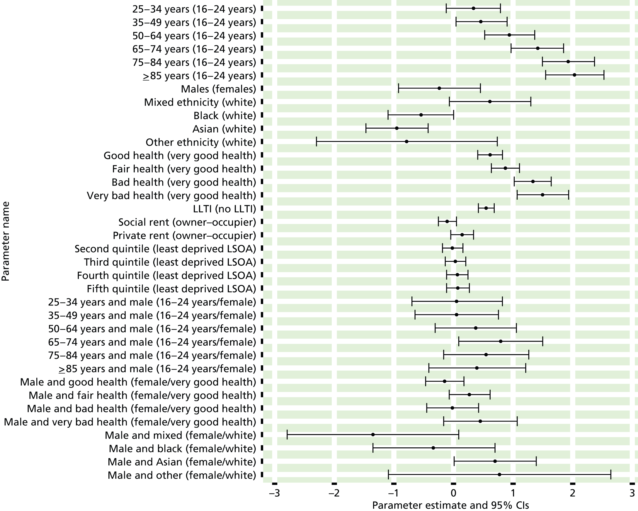
FIGURE 68.
Ever diagnosed with CVD: individual estimates and their 95% CIs. (a) MSOAs; (b) LAs; (c) CCGs; and (d) regions (GORs).


Ever been diagnosed with high blood pressure (Health Survey for England, 2006 and 2009–11)
FIGURE 69.
Ever diagnosed with high blood pressure: LSOA-level map. Contains Ordnance Survey data © Crown copyright and database right 2012.
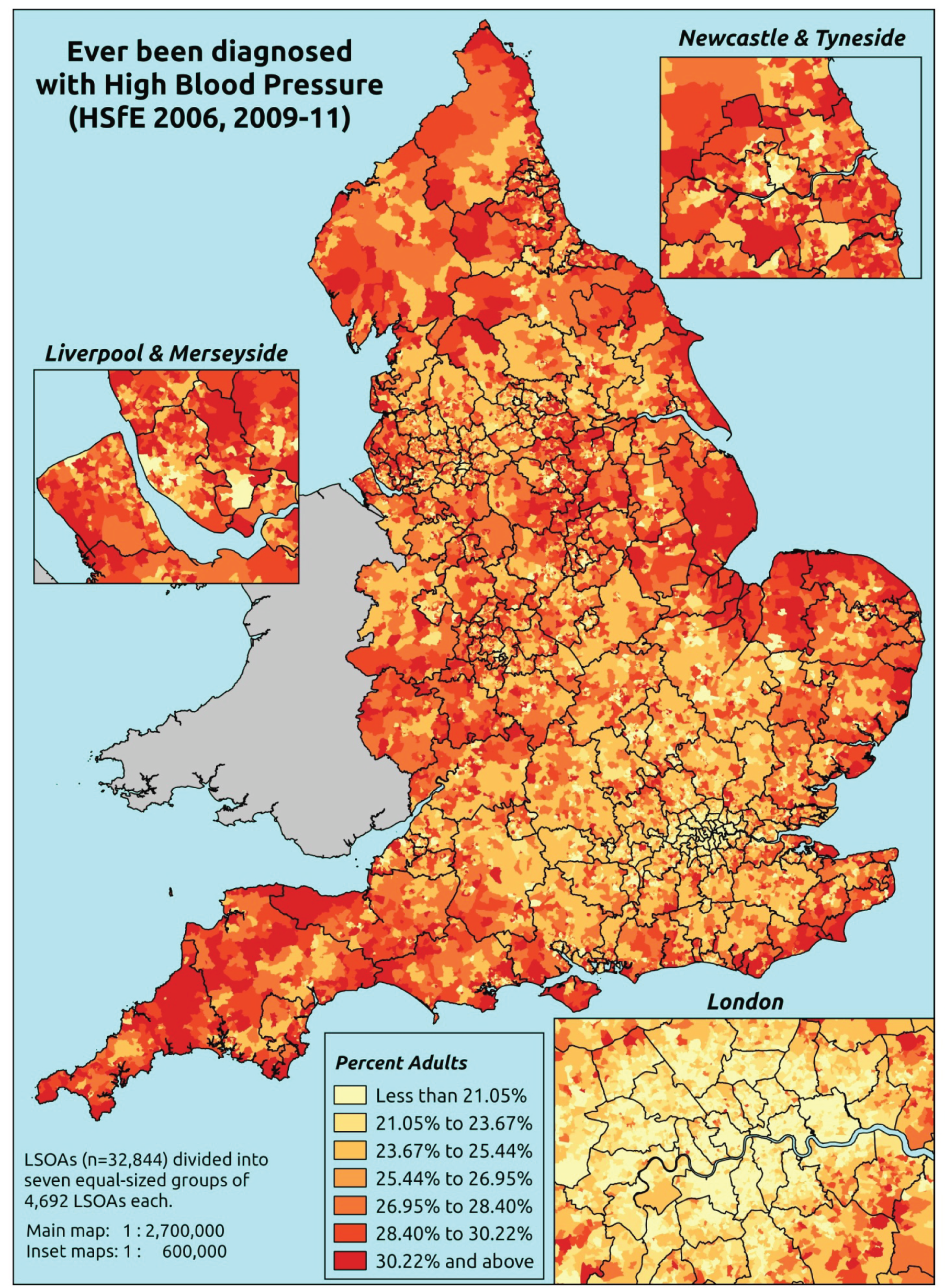
Response variable definition, provenance and prediction
These estimates are based on respondents to the HSfE reporting that they had ever been diagnosed with high blood pressure (hypertension).
The HSfE at this time includes multiple household respondents of all ages. The analytical data set is drawn from the subset of respondents aged ≥ 16 years for whom data are available across all model response and predictor variables, namely whether or not they responded to the question on doctor diagnosis of high blood pressure; whether or not they provided responses to questions on age, sex, ethnicity, general health status, LLTI and tenure; and whether or not information is available on the IMD quintile of their LSOA of residence (n = 33,872). To avoid a potential household-level effect, a single randomly selected adult is drawn from each household, resulting in an analytical data set of 18,641 adults aged ≥ 16 years.
| Age band (years) | Females | Age band (years) | Males | ||||
|---|---|---|---|---|---|---|---|
| Does not have condition | Has condition | % | Does not have condition | Has condition | % | ||
| 16–24 | 839 | 41 | 4.7 | 16–24 | 574 | 24 | 4.0 |
| 25–34 | 1653 | 117 | 6.6 | 25–34 | 997 | 116 | 10.4 |
| 35–49 | 2639 | 441 | 14.3 | 35–49 | 1862 | 377 | 16.8 |
| 50–64 | 1839 | 856 | 31.8 | 50–64 | 1350 | 791 | 36.9 |
| 65–74 | 561 | 567 | 50.3 | 65–74 | 485 | 473 | 49.4 |
| 75–84 | 399 | 548 | 57.9 | 75–84 | 249 | 320 | 56.2 |
| ≥ 85 | 157 | 194 | 55.3 | ≥ 85 | 100 | 72 | 41.9 |
| Females | 8087 | 2764 | 25.5 | Males | 5617 | 2173 | 27.9 |
| Total (males and females) | 13,704 | 4937 | 26.5 | ||||
Model parameters (see below) are applied to microsimulated LSOA-level census data to produce estimates of the number (and proportion) of people expected ever to have been diagnosed with high blood pressure (hypertension) in each age–sex cohort (and overall) in each of the 32,844 English LSOAs. As discussed in the report, bootstrapping is used to derive 95% CIs for these estimates. The bootstrapped LSOA-level prevalence rate estimates are aggregated into a number of higher geographies, namely for MSOAs, LAs, CCGs and regions (GORs), and are then used to calculate 95% CIs for these higher-level estimates. Proportionate attribution is used to restructure the estimates to align with 2001 MSOAs, as well as GP practice populations as defined by the 2011 NHS ADS.
Table 92 summarises how expected prevalence rates vary by age, sex and local deprivation (as measured by the 2010 IMD). There are 6569 LSOAs (with 9,226,227 adults) classified as being in the least deprived quintile; 6568 LSOAs (9,525,344 adults) in the second least deprived quintile; 6568 LSOAs (9,658,444 adults) in the third least deprived quintile; 6568 LSOAs (9,650,576 adults) in the fourth least deprived quintile; and 6568 LSOAs (9,535,167 adults) in the most deprived quintile. Note that, as a general rule, variations in prevalence rates reflect variations in the socioeconomic composition of populations in the different types of LSOA rather than variations in deprivation per se.
| Cohort | Least deprived quintile LSOAs | Second least deprived quintile LSOAs | Third least deprived quintile LSOAs | Fourth least deprived quintile LSOAs | Most deprived quintile LSOAs | All England |
|---|---|---|---|---|---|---|
| Female 16–24 | 3.5 (2.2 to 4.3) | 3.3 (2.2 to 4.3) | 4.0 (2.7 to 4.9) | 4.4 (3.0 to 5.3) | 4.4 (3.1 to 5.3) | 4.0 (2.8 to 4.8) |
| Female 25–34 | 4.8 (3.9 to 5.7) | 4.6 (3.8 to 5.6) | 5.5 (4.6 to 6.6) | 6.2 (5.0 to 7.3) | 6.2 (5.0 to 7.5) | 5.6 (4.7 to 6.6) |
| Female 35–49 | 12.2 (10.9 to 13.2) | 11.9 (10.8 to 13.3) | 14.4 (12.9 to 15.7) | 16.2 (14.6 to 17.7) | 16.7 (14.9 to 18.3) | 14.3 (13.2 to 15.2) |
| Female 50–64 | 29.5 (27.3 to 31.4) | 29.1 (26.6 to 31.6) | 33.6 (31.3 to 36.2) | 37.4 (34.6 to 39.7) | 39.1 (36.1 to 41.9) | 33.4 (31.7 to 35.0) |
| Female 65–74 | 47.4 (44.1 to 50.4) | 46.8 (44.0 to 49.9) | 51.9 (48.9 to 55.2) | 55.5 (52.3 to 58.9) | 56.3 (53.0 to 60.2) | 51.1 (48.4 to 53.7) |
| Female ≥ 75 | 55.3 (51.7 to 57.9) | 53.7 (50.6 to 56.5) | 58.1 (54.2 to 61.0) | 60.5 (56.3 to 63.3) | 59.6 (55.7 to 62.5) | 57.2 (54.3 to 59.4) |
| Females | 25.5 (23.4 to 27.2) | 24.7 (22.9 to 26.7) | 26.7 (24.6 to 28.7) | 26.6 (24.3 to 28.4) | 25.4 (23.2 to 27.4) | 25.8 (24.2 to 27.2) |
| Male 16–24 | 3.5 (2.2 to 4.8) | 3.3 (2.1 to 4.4) | 2.9 (1.9 to 3.9) | 3.8 (2.4 to 5.0) | 4.4 (2.8 to 5.8) | 3.7 (2.3 to 4.8) |
| Male 25–34 | 9.0 (7.7 to 10.7) | 8.4 (7.2 to 9.8) | 7.4 (6.2 to 8.8) | 9.5 (8.1 to 10.9) | 10.5 (8.9 to 12.8) | 9.1 (7.8 to 10.5) |
| Male 35–49 | 15.4 (13.8 to 17.5) | 14.8 (13.3 to 16.7) | 13.5 (12.1 to 15.4) | 17.4 (15.5 to 19.3) | 19.8 (17.9 to 22.0) | 16.2 (15.0 to 17.7) |
| Male 50–64 | 35.9 (33.6 to 38.7) | 35.1 (32.5 to 37.5) | 33.1 (30.4 to 35.6) | 40.4 (37.4 to 42.5) | 44.9 (42.0 to 47.7) | 37.6 (35.6 to 39.2) |
| Male 65–74 | 50.1 (45.6 to 53.2) | 48.9 (44.9 to 51.1) | 46.2 (42.6 to 49.3) | 53.5 (49.0 to 56.5) | 57.2 (53.0 to 61.0) | 50.7 (47.6 to 53.0) |
| Male ≥ 75 | 54.5 (49.9 to 58.8) | 52.6 (47.9 to 56.3) | 48.9 (44.9 to 52.6) | 55.7 (50.8 to 58.9) | 57.9 (53.2 to 61.5) | 53.6 (49.7 to 56.5) |
| Males | 27.6 (25.1 to 30.1) | 26.4 (24.0 to 28.5) | 23.3 (21.2 to 25.5) | 25.7 (23.2 to 27.6) | 26.7 (24.3 to 29.2) | 25.9 (24.0 to 27.6) |
| All | 26.5 (25.5 to 27.5) | 25.5 (24.3 to 26.4) | 25.1 (23.9 to 26.0) | 26.1 (25.1 to 27.0) | 26.0 (24.9 to 27.1) | 25.8 (25.2 to 26.3) |
| Factor (reference group) | Model coefficients | 95% CI | ||
|---|---|---|---|---|
| Estimate | Standard error | 2.5% CI | 97.50% | |
| (Intercept) | –4.01592 | 0.19792 | –4.40384 | –3.628 |
| Age (16–24 years) | ||||
| 25–34 years | 0.65131 | 0.21242 | 0.23496 | 1.06765 |
| 35–49 years | 1.53656 | 0.19441 | 1.15553 | 1.91760 |
| 50–64 years | 2.42000 | 0.19286 | 2.04200 | 2.79800 |
| 65–74 years | 3.18868 | 0.19965 | 2.79737 | 3.58000 |
| 75–84 years | 3.48406 | 0.20652 | 3.07927 | 3.88884 |
| ≥ 85 years | 3.44859 | 0.24348 | 2.97137 | 3.92581 |
| Sex (females) | ||||
| Males | 0.06927 | 0.27976 | –0.47906 | 0.61760 |
| Ethnicity (white) | ||||
| Mixed | 0.41128 | 0.19242 | 0.03415 | 0.78842 |
| Black | –0.19321 | 0.13361 | –0.45508 | 0.06866 |
| Asian | –0.16914 | 0.10204 | –0.36913 | 0.03085 |
| Other | –0.42425 | 0.30548 | –1.02300 | 0.17449 |
| General health status (very good) | ||||
| Good health | 0.71588 | 0.05361 | 0.61080 | 0.82096 |
| Fair health | 1.27450 | 0.07347 | 1.13050 | 1.41850 |
| Bad health | 1.44787 | 0.21776 | 1.02106 | 1.87469 |
| Very bad health | 1.60065 | 0.57179 | 0.47994 | 2.72135 |
| LLTI (no LTTI) | ||||
| LLTI | 1.65205 | 0.31502 | 1.03462 | 2.26949 |
| Tenure (owner–occupier) | ||||
| Social rent | 0.09992 | 0.05334 | –0.00463 | 0.20446 |
| Private rent or other tenure | –0.03512 | 0.06766 | –0.16774 | 0.09749 |
| LSOA deprivation quintile (least deprived quintile) | ||||
| Second quintile | –0.08134 | 0.07765 | –0.23354 | 0.07086 |
| Third quintile | 0.07546 | 0.07788 | –0.07719 | 0.22811 |
| Fourth quintile | 0.15328 | 0.07883 | –0.00122 | 0.30778 |
| Fifth quintile ( = most deprived quintile) | 0.07654 | 0.08424 | –0.08858 | 0.24166 |
| Interaction effects | ||||
| 25–34 years and LLTI (16–24 years/no LLTI) | –1.06141 | 0.33181 | –1.71175 | –0.41106 |
| 35–49 years and LLTI (16–24 years/no LLTI) | –1.25514 | 0.29840 | –1.84001 | –0.67027 |
| 50–64 years and LLTI (16–24 years/no LLTI) | –1.09377 | 0.29234 | –1.66675 | –0.52079 |
| 65–74 years and LLTI (16–24 years/no LLTI) | –1.25582 | 0.29927 | –1.84239 | –0.66925 |
| 75–84 years and LLTI (16–24 years/no LLTI) | –1.48607 | 0.30406 | –2.08202 | –0.89012 |
| ≥ 85 years and LLTI (16–24 years/no LLTI) | –1.57558 | 0.33888 | –2.23979 | –0.91137 |
| 25–34 years and male (16–24 years/female) | 0.60545 | 0.30187 | 0.01378 | 1.19711 |
| 35–49 years and male (16–24 years/female) | 0.23200 | 0.27926 | –0.31534 | 0.77935 |
| 50–64 years and male (16–24 years/female) | 0.24697 | 0.27577 | –0.29354 | 0.78749 |
| 65–74 years and male (16–24 years/female) | 0.02876 | 0.28345 | –0.52680 | 0.58432 |
| 75–84 years and male (16–24 years/female) | 0.04788 | 0.29011 | –0.52074 | 0.61649 |
| ≥ 85 years and male (16–24 years/female) | –0.56382 | 0.33144 | –1.21345 | 0.08581 |
| Male and second quintile (female/least deprived) | –0.02138 | 0.11597 | –0.24867 | 0.20591 |
| Male and third quintile (female/least deprived) | –0.33915 | 0.11674 | –0.56796 | –0.11034 |
| Male and fourth quintile (female/least deprived) | –0.17873 | 0.11781 | –0.40964 | 0.05219 |
| Male and fifth quintile (female/least deprived) | –0.04316 | 0.12058 | –0.27950 | 0.19319 |
| Good health and LLTI (very good health/no LLTI) | –0.32453 | 0.16060 | –0.63931 | –0.00976 |
| Fair health and LLTI (very good health/no LLTI) | –0.50289 | 0.16353 | –0.82341 | –0.18237 |
| Bad health and LLTI (very good health/no LLTI) | –0.51113 | 0.26628 | –1.03304 | 0.01078 |
| Very bad health and LLTI (very good health/no LLTI) | –0.56302 | 0.59880 | –1.73667 | 0.61063 |
FIGURE 70.
Parameter plots: ever diagnosed with high blood pressure.

FIGURE 71.
Ever diagnosed with high blood pressure: individual estimates and their 95% CIs. (a) MSOAs; (b) LAs; (c) CCGs; and (d) regions (GORs). BP, blood pressure.


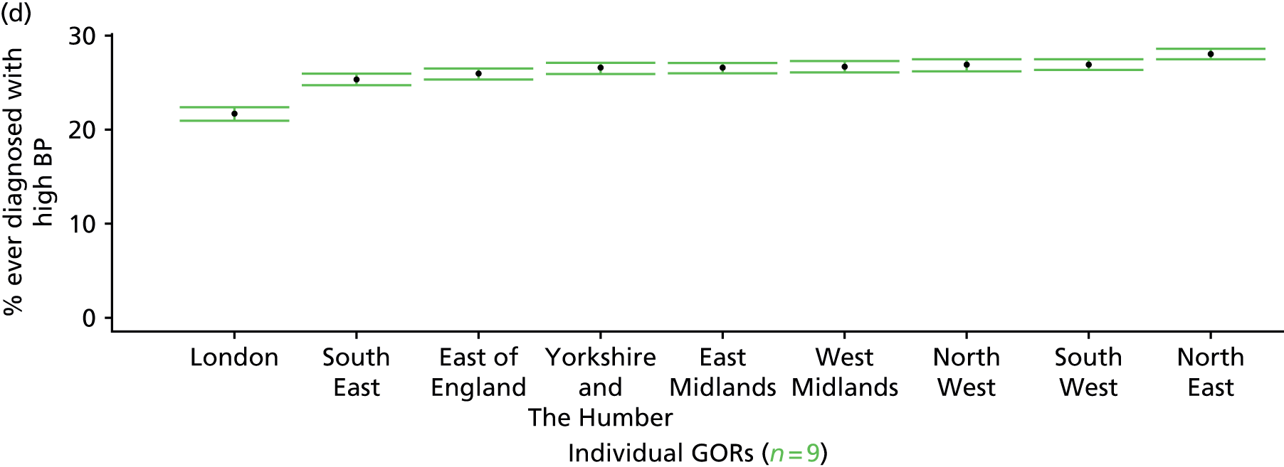
Ever been diagnosed with diabetes (Health Survey for England, 2006 and 2009–11)
FIGURE 72.
Ever diagnosed with diabetes: LSOA-level map. Contains Ordnance Survey data © Crown copyright and database right 2012.
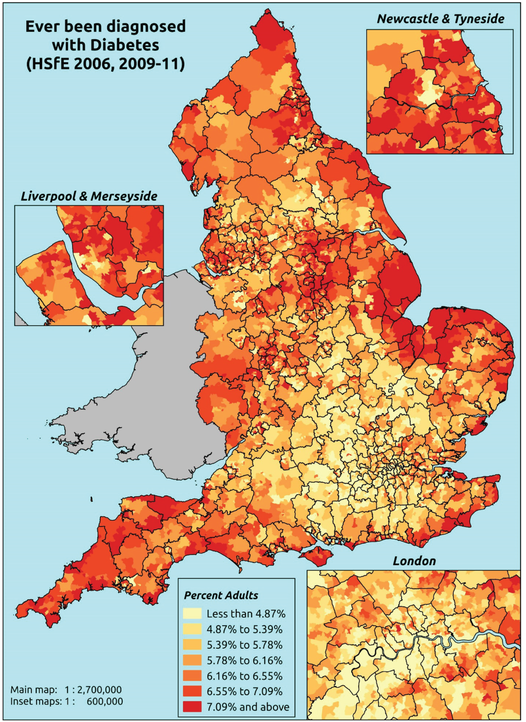
Response variable definition, provenance and prediction
These estimates are based on respondents to the HSfE reporting whether or not they had ever been diagnosed with diabetes.
The HSfE at this time includes multiple household respondents of all ages. The analytical data set is drawn from the subset of respondents aged ≥ 16 years for whom data are available across all model response and predictor variables, namely: whether they responded to the question on doctor diagnosis diabetes; whether they provided responses to questions on age, sex, ethnicity, general health status, LLTI and tenure; and whether information is available on the IMD quintile of their LSOA of residence (n = 33,938). To avoid a potential household-level effect, a single randomly selected adult is drawn from each household, resulting in an analytical data set of 12,803 adults aged > 16 years.
| Age band (years) | Females | Age band (years) | Males | ||||
|---|---|---|---|---|---|---|---|
| Does not have condition | Has condition | % | Does not have condition | Has condition | % | ||
| 16–24 | 876 | 4 | 0.5 | 16–24 | 599 | 5 | 0.8 |
| 25–34 | 1749 | 25 | 1.4 | 25–34 | 1104 | 13 | 1.2 |
| 35–49 | 3021 | 64 | 2.1 | 35–49 | 2175 | 69 | 3.1 |
| 50–64 | 2537 | 158 | 5.9 | 50–64 | 1959 | 185 | 8.6 |
| 65–74 | 1012 | 121 | 10.7 | 65–74 | 823 | 135 | 14.1 |
| 75–84 | 813 | 136 | 14.3 | 75–84 | 477 | 95 | 16.6 |
| ≥ 85 | 314 | 38 | 10.8 | ≥ 85 | 149 | 28 | 15.8 |
| Females | 10,322 | 546 | 5.0 | Males | 7286 | 530 | 6.8 |
| Total (males and females) | 17,608 | 1076 | 5.8 | ||||
Model parameters (see below) are applied to microsimulated LSOA-level census data to produce estimates of the number (and proportion) of people expected ever to have been diagnosed with diabetes in each age–sex cohort (and overall) in each of the 32,844 English LSOAs. As discussed in the report, bootstrapping is used to derive 95% CIs for these estimates. The bootstrapped LSOA-level prevalence rate estimates are aggregated into a number of higher geographies, namely for MSOAs, LAs, CCGs and regions (GORs), and are then used to calculate 95% CIs for these higher-level estimates. Proportionate attribution is used to restructure the estimates to align with 2001 MSOAs, as well as GP practice populations as defined by the 2011 NHS ADS.
Table 95 summarises how expected prevalence rates vary by age, sex and local deprivation (as measured by the 2010 IMD). There are 6569 LSOAs (with 9,226,227 adults) classified as being in the least deprived quintile; 6568 LSOAs (9,525,344 adults) in the second least deprived quintile; 6568 LSOAs (9,658,444 adults) in the third least deprived quintile; 6568 LSOAs (9,650,576 adults) in the fourth least deprived quintile; and 6568 LSOAs (9,535,167 adults) in the most deprived quintile. Note that, as a general rule, variations in prevalence rates reflect variations in the socioeconomic composition of populations in the different types of LSOA rather than variations in deprivation per se.
| Cohort | Least deprived quintile LSOAs | Second least deprived quintile LSOAs | Third least deprived quintile LSOAs | Fourth least deprived quintile LSOAs | Most deprived quintile LSOAs | All England |
|---|---|---|---|---|---|---|
| Female 16–24 | 0.3 (0.1 to 0.5) | 0.3 (0.1 to 0.5) | 0.3 (0.2 to 0.6) | 0.4 (0.2 to 0.7) | 0.4 (0.2 to 0.7) | 0.3 (0.2 to 0.6) |
| Female 25–34 | 0.6 (0.4 to 0.8) | 0.7 (0.5 to 0.9) | 0.8 (0.6 to 1.1) | 0.9 (0.7 to 1.3) | 1.1 (0.8 to 1.4) | 0.9 (0.6 to 1.1) |
| Female 35–49 | 1.3 (1.1 to 1.5) | 1.6 (1.3 to 1.9) | 1.9 (1.6 to 2.4) | 2.4 (2.0 to 2.9) | 2.9 (2.4 to 3.5) | 2.0 (1.7 to 2.4) |
| Female 50–64 | 4.4 (3.7 to 5.1) | 5.2 (4.5 to 6.0) | 6.2 (5.3 to 7.3) | 7.8 (6.6 to 8.8) | 9.4 (8.0 to 10.9) | 6.4 (5.7 to 7.2) |
| Female 65–74 | 8.6 (7.4 to 10.1) | 10.0 (8.7 to 11.7) | 11.5 (10.3 to 13.7) | 14.0 (12.0 to 15.9) | 16.2 (14.1 to 18.5) | 11.7 (10.5 to 13.1) |
| Female ≥ 75 | 12.6 (10.8 to 14.3) | 14.0 (12.5 to 16.1) | 15.4 (13.6 to 17.8) | 17.5 (15.3 to 19.8) | 18.8 (16.0 to 21.6) | 15.5 (14.1 to 17.2) |
| Females | 4.4 (3.7 to 5.2) | 5.1 (4.4 to 5.9) | 5.5 (4.8 to 6.6) | 6.0 (5.1 to 6.9) | 6.4 (5.4 to 7.4) | 5.5 (4.9 to 6.2) |
| Male 16–24 | 0.4 (0.2 to 0.7) | 0.4 (0.2 to 0.8) | 0.5 (0.2 to 0.9) | 0.5 (0.3 to 0.9) | 0.6 (0.3 to 1.0) | 0.5 (0.2 to 0.9) |
| Male 25–34 | 1.0 (0.7 to 1.3) | 1.1 (0.7 to 1.4) | 1.2 (0.8 to 1.6) | 1.3 (0.9 to 1.8) | 1.5 (1.0 to 2.0) | 1.2 (0.9 to 1.6) |
| Male 35–49 | 2.1 (1.6 to 2.4) | 2.3 (1.9 to 2.8) | 2.7 (2.2 to 3.2) | 3.2 (2.6 to 3.8) | 3.6 (3.0 to 4.3) | 2.8 (2.4 to 3.2) |
| Male 50–64 | 6.6 (5.5 to 7.5) | 7.5 (6.3 to 8.4) | 8.6 (7.4 to 9.9) | 10.0 (8.4 to 11.2) | 11.1 (9.3 to 12.5) | 8.6 (7.5 to 9.4) |
| Male 65–74 | 12.3 (10.4 to 14.3) | 13.9 (12.0 to 15.7) | 15.4 (13.4 to 17.6) | 17.6 (15.1 to 19.6) | 18.7 (16.1 to 21.1) | 15.3 (13.7 to 16.9) |
| Male ≥ 75 | 16.3 (13.9 to 18.4) | 17.7 (15.3 to 20.1) | 18.8 (17.0 to 21.9) | 20.7 (17.7 to 23.2) | 21.1 (18.1 to 24.1) | 18.7 (16.7 to 20.8) |
| Males | 5.9 (4.9 to 6.8) | 6.5 (5.5 to 7.4) | 6.7 (5.8 to 7.9) | 6.9 (5.7 to 7.8) | 6.9 (5.8 to 7.9) | 6.6 (5.7 to 7.3) |
| All | 5.1 (4.5 to 5.7) | 5.7 (5.2 to 6.4) | 6.1 (5.5 to 6.9) | 6.4 (5.7 to 6.9) | 6.6 (5.9 to 7.3) | 6.0 (5.6 to 6.4) |
| Factor (reference group) | Model coefficients | 95% CI | ||
|---|---|---|---|---|
| Estimate | Standard error | 2.5% CI | 97.50% | |
| (Intercept) | –6.72943 | 0.40065 | –7.5147 | –5.94415 |
| Age (16–24 years) | ||||
| 25–34 years | 0.79918 | 0.37558 | 0.06304 | 1.53532 |
| 35–49 years | 1.36594 | 0.35022 | 0.67951 | 2.05237 |
| 50–64 years | 2.27291 | 0.34557 | 1.59559 | 2.95022 |
| 65–74 years | 2.79441 | 0.34813 | 2.11207 | 3.47676 |
| 75–84 years | 2.87961 | 0.34994 | 2.19372 | 3.56549 |
| ≥ 85 years | 2.64843 | 0.36834 | 1.92649 | 3.37038 |
| Sex (females) | ||||
| Males | 0.62141 | 0.25880 | 0.11416 | 1.12866 |
| Ethnicity (white) | ||||
| Mixed | –0.09266 | 0.60962 | –1.28751 | 1.10220 |
| Black | –0.17116 | 0.40441 | –0.96380 | 0.62148 |
| Asian | 1.19225 | 0.15974 | 0.87916 | 1.50534 |
| Other | –0.39234 | 1.04187 | –2.43442 | 1.64973 |
| General health status (very good) | ||||
| Good health | 0.93496 | 0.22605 | 0.49190 | 1.37802 |
| Fair health | 1.92701 | 0.22659 | 1.48289 | 2.37113 |
| Bad health | 2.45986 | 0.25109 | 1.96772 | 2.95199 |
| Very bad health | 2.64725 | 0.32004 | 2.01997 | 3.27453 |
| LLTI (no LTTI) | ||||
| LLTI | 0.27487 | 0.08256 | 0.11305 | 0.43669 |
| Tenure (owner–occupier) | ||||
| Social rent | –0.05812 | 0.53041 | –1.09773 | 0.98149 |
| Private rent or other tenure | –0.30183 | 0.54936 | –1.37857 | 0.77491 |
| LSOA deprivation quintile (least deprived quintile) | ||||
| Second quintile | 0.04589 | 0.11080 | –0.17127 | 0.26305 |
| Third quintile | 0.07768 | 0.11039 | –0.13869 | 0.29405 |
| Fourth quintile | 0.11818 | 0.11210 | –0.10154 | 0.33790 |
| Fifth quintile ( = most deprived quintile) | 0.05295 | 0.11814 | –0.17860 | 0.28450 |
| Interaction effects | ||||
| Mixed and social rent (white/owner–occupier) | –12.0283 | 207.1847 | –418.110 | 394.0536 |
| Black and social rent (white/owner–occupier) | 0.72275 | 0.49589 | –0.24919 | 1.69469 |
| Asian and social rent (white/owner–occupier) | –1.46816 | 0.50682 | –2.46153 | –0.47479 |
| Other and social rent (white/owner–occupier) | –11.6280 | 225.5789 | –453.763 | 430.5065 |
| Mixed and private rent (white/owner–occupier) | 2.25433 | 0.81040 | 0.66593 | 3.84272 |
| Black and private rent (white/owner–occupier) | 0.80492 | 0.74606 | –0.65736 | 2.26719 |
| Asian and private rent (white/owner–occupier) | –0.98010 | 0.57752 | –2.11204 | 0.15185 |
| Other and private rent (white/owner–occupier) | 2.04220 | 1.26422 | –0.43568 | 4.52007 |
| Male and social rent (female/owner–occupier) | –0.42674 | 0.15789 | –0.73622 | –0.11727 |
| Male and private rent (female/owner–occupier) | –0.13990 | 0.26818 | –0.66553 | 0.38573 |
| Male and good health (female/very good health) | 0.10323 | 0.28515 | –0.45566 | 0.66212 |
| Male and fair health (female/very good health) | –0.16437 | 0.28177 | –0.71664 | 0.38790 |
| Male and bad health (female/very good health) | –0.45086 | 0.30932 | –1.05713 | 0.15541 |
| Male and very bad health (female/very good health) | –0.63977 | 0.38064 | –1.38583 | 0.10629 |
| Good health and social rent (very good health/owner–occupier) | 0.97254 | 0.54280 | –0.09134 | 2.03643 |
| Fair health and social rent (very good health/owner–occupier) | 0.41461 | 0.53856 | –0.64098 | 1.47019 |
| Bad health and social rent (very good health/owner–occupier) | 0.31003 | 0.55189 | –0.77167 | 1.39172 |
| Very bad health and social rent (very good health/owner–occupier) | 0.45328 | 0.59201 | –0.70705 | 1.61361 |
| Good health and private rent (very good health/owner–occupier) | –0.07428 | 0.57979 | –1.21068 | 1.06211 |
| Fair health and private rent (very good health/owner–occupier) | 0.72490 | 0.55793 | –0.36864 | 1.81844 |
| Bad health and private rent (very good health/owner–occupier) | –0.04107 | 0.62283 | –1.26182 | 1.17968 |
| Very bad health and private rent (very good health/owner–occupier) | 0.11091 | 0.79381 | –1.44496 | 1.66679 |
FIGURE 73.
Parameter plots: ever diagnosed with diabetes.
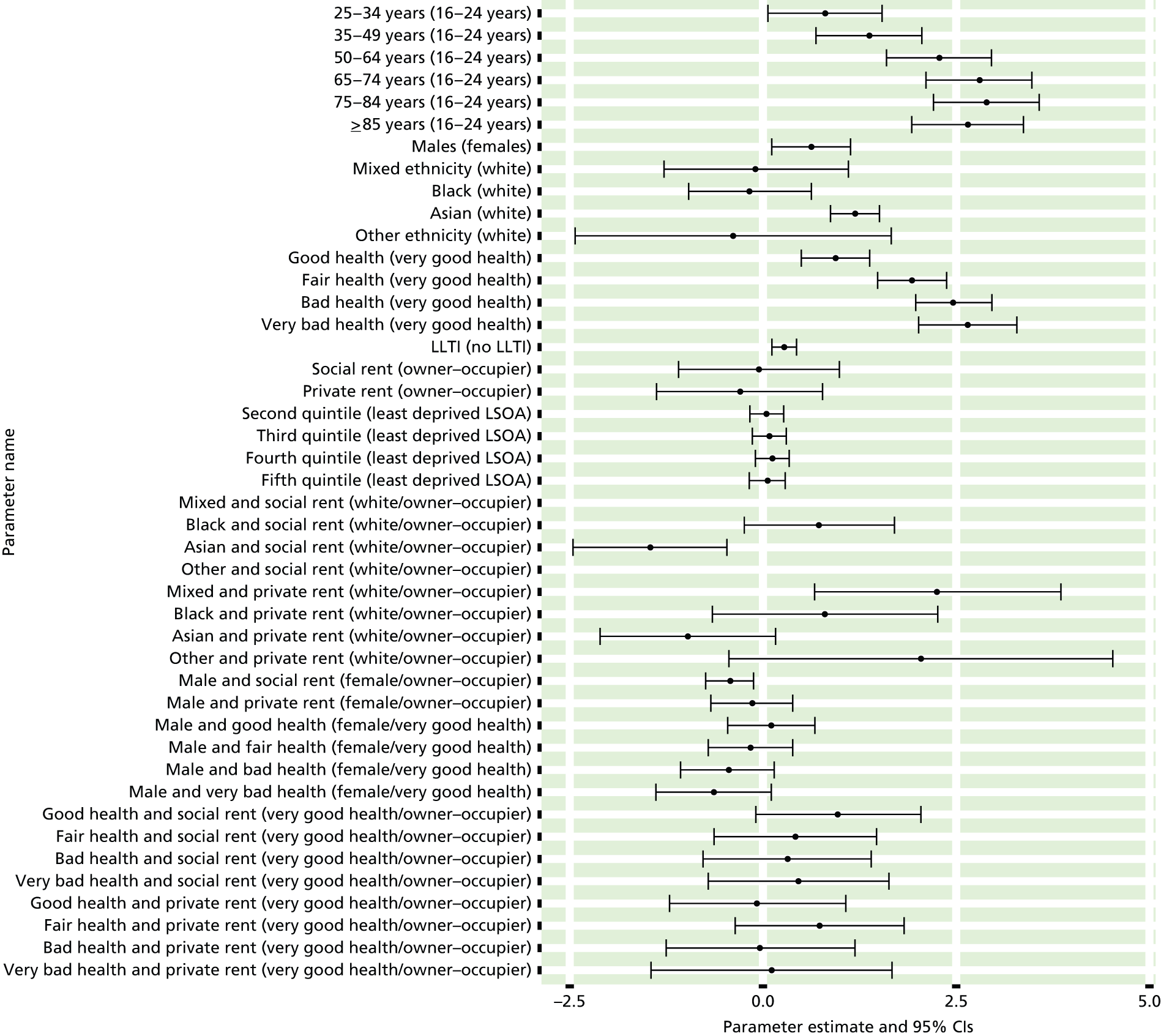
FIGURE 74.
Ever diagnosed with diabetes: individual estimates and their 95% CIs. (a) MSOAs; (b) LAs; (c) CCGs; and (d) regions (GORs).


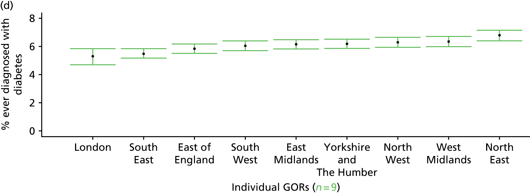
Diagnosed and undiagnosed diabetes (Health Survey for England, 2006 and 2009–11)
FIGURE 75.
Diagnosed and undiagnosed diabetes: LSOA-level map. Contains Ordnance Survey data © Crown copyright and database right 2012.
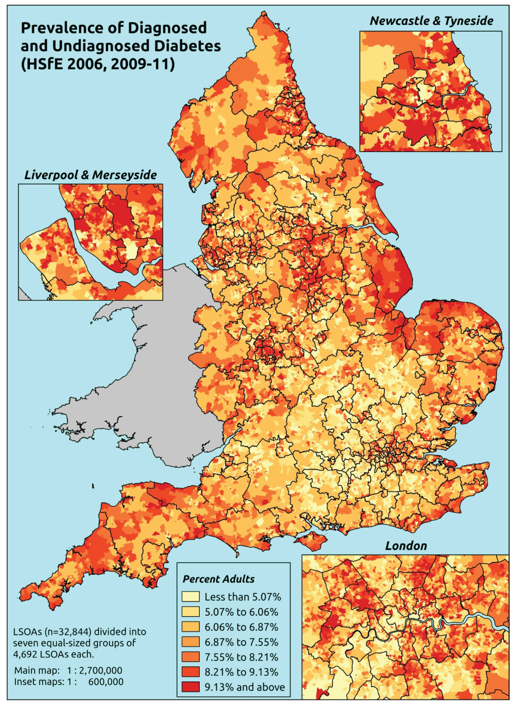
Response variable definition, provenance and prediction
These estimates are based on respondents to the HSfE reporting whether they have ever been diagnosed with diabetes and whether or not their nurse-administered blood sample returns a glycated haemoglobin value of ≥ 6.5%. The latter should capture undiagnosed diabetes.
The HSfE at this time includes multiple household respondents of all ages. The analytical data set is drawn from the subset of respondents aged ≥ 16 years for whom data are available for both doctor diagnoses and the glycated haemoglobin blood test, as well as in response to questions on age, sex, ethnicity, general health status, LLTI and tenure and whether information is available on the IMD quintile of their LSOA of residence (n = 16,523). To avoid a potential household-level effect, a single randomly selected adult is drawn from each household, resulting in an analytical data set of 11,061 adults aged ≥ 16 years.
| Age band (years) | Females | Age band (years) | Males | ||||
|---|---|---|---|---|---|---|---|
| Does not have condition | Has condition | % | Does not have condition | Has condition | % | ||
| 16–24 | 343 | 2 | 0.6 | 16–24 | 273 | 5 | 1.8 |
| 25–34 | 787 | 6 | 0.8 | 25–34 | 660 | 12 | 1.8 |
| 35–49 | 1906 | 43 | 2.2 | 35–49 | 1438 | 39 | 2.6 |
| 50–64 | 1706 | 118 | 6.5 | 50–64 | 1283 | 147 | 10.3 |
| 65–74 | 646 | 79 | 10.9 | 65–74 | 494 | 95 | 16.1 |
| 75–84 | 378 | 67 | 15.1 | 75–84 | 254 | 58 | 18.6 |
| ≥ 85 | 129 | 16 | 11.0 | ≥ 85 | 59 | 18 | 23.4 |
| Females | 5895 | 331 | 5.3 | Males | 4461 | 374 | 7.7 |
| Total (males and females) | 10,356 | 705 | 6.4 | ||||
Model parameters (see below) are applied to microsimulated LSOA-level census data to produce estimates of the number (and proportion) of people expected have diagnosed or undiagnosed diabetes in each age–sex cohort (and overall) in each of the 32,844 English LSOAs. As discussed in the report, bootstrapping is used to derive 95% CIs for these estimates. The bootstrapped LSOA-level prevalence rate estimates are aggregated into a number of higher geographies, namely for MSOAs, LAs, CCGs and regions (GORs), and are then used to calculate 95% CIs for these higher-level estimates. Proportionate attribution is used to restructure the estimates to align with 2001 MSOAs, as well as GP practice populations as defined by the 2011 NHS ADS.
Table 98 summarises how expected prevalence rates vary by age, sex and local deprivation (as measured by the 2010 IMD). There are 6569 LSOAs (with 9,226,227 adults) classified as being in the least deprived quintile; 6568 LSOAs (9,525,344 adults) in the second least deprived quintile; 6568 LSOAs (9,658,444 adults) in the third least deprived quintile; 6568 LSOAs (9,650,576 adults) in the fourth least deprived quintile; and 6568 LSOAs (9,535,167 adults) in the most deprived quintile. Note that, as a general rule, variations in prevalence rates reflect variations in the socioeconomic composition of populations in the different types of LSOA rather than variations in deprivation per se.
| Cohort | Least deprived quintile LSOAs | Second least deprived quintile LSOAs | Third least deprived quintile LSOAs | Fourth least deprived quintile LSOAs | Most deprived quintile LSOAs | All England |
|---|---|---|---|---|---|---|
| Female 16–24 | 0.4 (0.2 to 0.6) | 0.6 (0.2 to 0.9) | 0.6 (0.3 to 0.9) | 0.8 (0.3 to 1.2) | 0.9 (0.4 to 1.5) | 0.7 (0.3 to 1.0) |
| Female 25–34 | 0.5 (0.3 to 0.7) | 0.6 (0.5 to 0.9) | 0.7 (0.5 to 0.9) | 0.9 (0.6 to 1.2) | 1.2 (0.8 to 1.5) | 0.8 (0.6 to 1.1) |
| Female 35–49 | 1.1 (0.8 to 1.3) | 1.6 (1.3 to 2.0) | 1.8 (1.4 to 2.1) | 2.5 (2.0 to 3.0) | 3.4 (2.6 to 4.1) | 2.1 (1.7 to 2.4) |
| Female 50–64 | 4.4 (3.5 to 5.1) | 6.3 (5.3 to 7.6) | 7.0 (5.9 to 8.2) | 9.5 (7.6 to 10.8) | 12.3 (10.2 to 14.4) | 7.7 (6.6 to 8.6) |
| Female 65–74 | 8.3 (6.7 to 9.6) | 11.6 (10.0 to 13.9) | 12.5 (10.4 to 14.4) | 16.3 (13.6 to 18.6) | 20.2 (16.7 to 23.2) | 13.3 (11.5 to 14.9) |
| Female ≥ 75 | 11.4 (9.3 to 12.8) | 15.5 (13.3 to 18.3) | 16.0 (13.3 to 18.3) | 19.5 (16.4 to 21.6) | 22.4 (18.8 to 25.7) | 16.6 (14.8 to 18.3) |
| Females | 4.2 (3.3 to 4.8) | 5.8 (4.9 to 7.0) | 5.9 (4.9 to 6.9) | 6.9 (5.6 to 7.9) | 7.9 (6.4 to 9.3) | 6.1 (5.3 to 6.9) |
| Male 16–24 | 0.6 (0.3 to 1.1) | 0.9 (0.4 to 1.5) | 0.9 (0.4 to 1.5) | 1.1 (0.5 to 1.9) | 1.3 (0.5 to 2.1) | 1.0 (0.4 to 1.6) |
| Male 25–34 | 0.8 (0.5 to 1.1) | 1.1 (0.8 to 1.6) | 1.1 (0.8 to 1.5) | 1.3 (0.9 to 1.9) | 1.6 (1.1 to 2.2) | 1.2 (0.9 to 1.7) |
| Male 35–49 | 1.8 (1.3 to 2.1) | 2.6 (2.1 to 3.2) | 2.8 (2.2 to 3.3) | 3.6 (2.9 to 4.4) | 4.6 (3.7 to 5.5) | 3.1 (2.6 to 3.5) |
| Male 50–64 | 7.3 (6.1 to 8.4) | 10.2 (9.0 to 11.9) | 11.0 (9.4 to 12.4) | 13.8 (11.6 to 15.3) | 16.5 (14.4 to 18.8) | 11.5 (10.2 to 12.7) |
| Male 65–74 | 13.5 (11.2 to 15.4) | 18.3 (15.9 to 21.6) | 19.2 (16.0 to 21.8) | 23.3 (19.7 to 25.9) | 26.8 (22.9 to 30.0) | 19.7 (17.1 to 21.7) |
| Male ≥ 75 | 17.9 (14.2 to 20.0) | 23.4 (20.4 to 26.8) | 23.8 (20.5 to 26.8) | 27.8 (23.4 to 30.8) | 30.9 (26.4 to 34.2) | 24.2 (21.1 to 26.3) |
| Males | 6.3 (5.1 to 7.3) | 8.5 (7.3 to 10.0) | 8.3 (6.9 to 9.5) | 9.0 (7.4 to 10.3) | 9.8 (8.3 to 11.3) | 8.4 (7.2 to 9.4) |
| All | 5.2 (4.4 to 5.8) | 7.1 (6.4 to 8.1) | 7.1 (6.2 to 7.9) | 7.9 (6.9 to 8.6) | 8.8 (7.8 to 9.8) | 7.2 (6.7 to 7.6) |
| Factor (reference group) | Model coefficients | 95% CI | ||
|---|---|---|---|---|
| Estimate | Standard error | 2.5% CI | 97.50% | |
| (Intercept) | –6.16878 | 0.42144 | –6.99479 | –5.34276 |
| Age (16–24 years) | ||||
| 25–34 years | 0.07655 | 0.45136 | –0.80812 | 0.96122 |
| 35–49 years | 0.74444 | 0.40062 | –0.04078 | 1.52965 |
| 50–64 years | 1.92090 | 0.39229 | 1.15202 | 2.68978 |
| 65–74 years | 2.45388 | 0.39678 | 1.67620 | 3.23156 |
| 75–84 years | 2.55626 | 0.40142 | 1.76947 | 3.34305 |
| ≥ 85 years | 2.43772 | 0.43313 | 1.58879 | 3.28665 |
| Sex (females) | ||||
| Males | 0.61605 | 0.09904 | 0.42193 | 0.81017 |
| Ethnicity (white) | ||||
| Mixed | 0.86711 | 0.48180 | –0.07722 | 1.81144 |
| Black | –0.60419 | 0.60196 | –1.78403 | 0.57565 |
| Asian | 0.94024 | 0.24956 | 0.45110 | 1.42938 |
| Other | –11.4344 | 209.8598 | –422.760 | 399.8908 |
| General health status (very good) | ||||
| Good health | 0.89613 | 0.15749 | 0.58745 | 1.20480 |
| Fair health | 1.90906 | 0.17222 | 1.57151 | 2.24661 |
| Bad health | 1.52785 | 0.50193 | 0.54406 | 2.51164 |
| Very bad health | 1.89427 | 1.09476 | –0.25147 | 4.04001 |
| LLTI (no LTTI) | ||||
| LLTI | 0.11273 | 0.47701 | –0.82222 | 1.04768 |
| Tenure (owner–occupier) | ||||
| Social rent | 0.55847 | 0.14227 | 0.27963 | 0.83732 |
| Private rent or other tenure | –0.16193 | 0.25889 | –0.66936 | 0.34550 |
| LSOA deprivation quintile (least deprived quintile) | ||||
| Second quintile | 0.29119 | 0.13696 | 0.02276 | 0.55963 |
| Third quintile | 0.24200 | 0.13985 | –0.03211 | 0.51611 |
| Fourth quintile | 0.35292 | 0.14060 | 0.07734 | 0.62850 |
| Fifth quintile ( = most deprived quintile) | 0.35127 | 0.14973 | 0.05781 | 0.64474 |
| Interaction effects | ||||
| Male and social rent (female/owner–occupier) | –0.57532 | 0.20061 | –0.96851 | –0.18213 |
| Male and private rent (female/owner–occupier) | 0.14822 | 0.33727 | –0.51284 | 0.80928 |
| Mixed and LLTI (white/no LLTI) | 0.13357 | 0.83441 | –1.50187 | 1.76901 |
| Black and LLTI (white/no LLTI) | 1.92048 | 0.75459 | 0.44147 | 3.39948 |
| Asian and LLTI (white/no LLTI) | 0.39243 | 0.38419 | –0.36059 | 1.14545 |
| Other and LLTI (white/no LLTI) | 12.06304 | 209.8629 | –399.268 | 423.3942 |
| Good health and LLTI (very good health/no LLTI) | 0.30628 | 0.49966 | –0.67305 | 1.28561 |
| Fair health and LLTI (very good health/no LLTI) | –0.26503 | 0.49575 | –1.23671 | 0.70664 |
| Bad health and LLTI (very good health/no LLTI) | 0.49725 | 0.68799 | –0.85120 | 1.84571 |
| Very bad health and LLTI (very good health/no LLTI) | 0.18655 | 1.20929 | –2.18366 | 2.55676 |
FIGURE 76.
Parameter plots: diagnosed and undiagnosed diabetes.
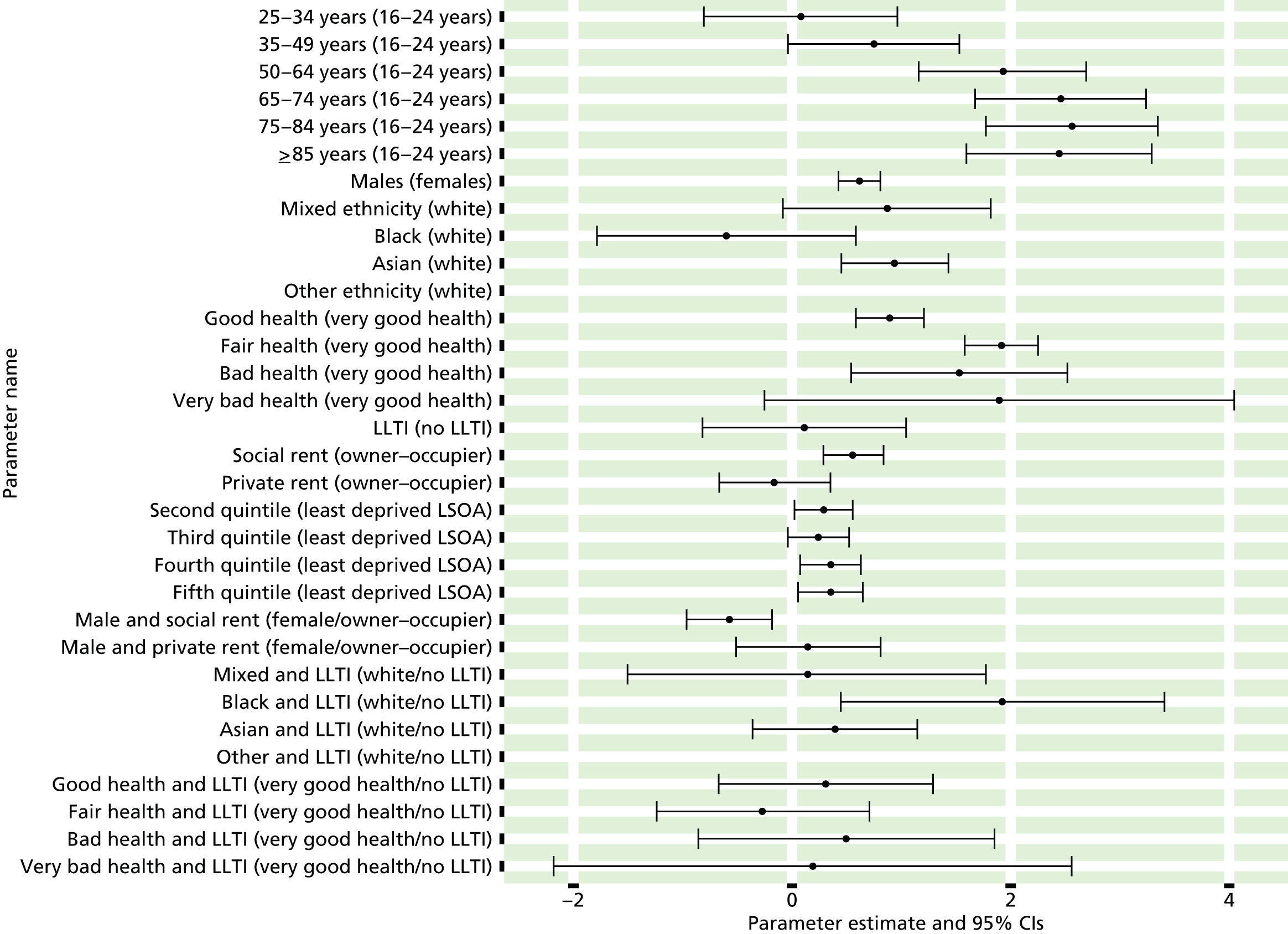
FIGURE 77.
Diagnosed and undiagnosed diabetes: individual estimates and their 95% CIs: (a) MSOAs; (b) LAs; (c) CCGs; and (d) regions (GORs).


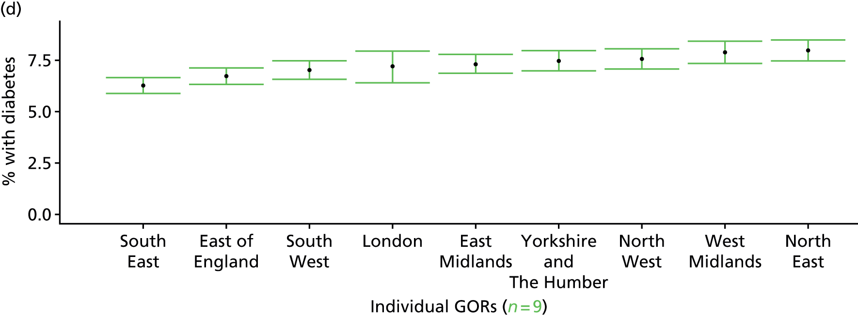
Adults 25–74 years with ≥ 10% risk of coronary heart disease in next 10 years (Health Survey for England, 2006 and 2009–11)
FIGURE 78.
Adults 25–74 years with ≥ 10% risk of CHD in next 10 years: LSOA-level map. Contains Ordnance Survey data © Crown copyright and database right 2012.
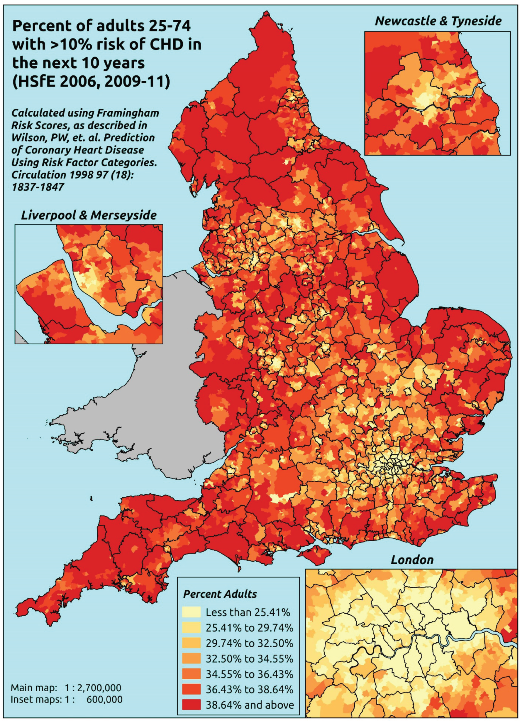
Response variable definition, provenance and prediction
Estimates of the proportion of adults aged 25–74 years with a ≥ 10% risk of developing CHD in the next 10 years are based on HSfE data on respondents’ age, sex, cholesterol levels (total and high-density lipoprotein), blood pressure, whether or not they have diagnosed or undiagnosed diabetes and whether or not they smoke. Using the methodology described in Wilson et al. ,502 each respondent’s risk of developing CHD over the next 10 years is calculated. A generalised linear model for binomial data with a logistic link is used to model whether or not individuals have/do not have a ≥ 10% risk of developing CHD over the next 10 years, using the usual set of sociodemographic predictor variables.
The methodology described by Wilson et al. 502 was developed by analysing data from the Framingham Heart Study on 2489 men and 2856 women aged 30–74 years at baseline (1971–74). These individuals were followed for 12 years and the data were used to construct the Framingham Risk calculator, a methodology for assessing the risk of developing CHD over the next 10 years.
There are shortcomings, not least the lack of ethnicity in the algorithm, and more recent risk calculators have been developed, including QRISK® (ClinRisk Ltd, University of Nottingham/EMIS; www.qrisk.org/index.php). Moreover, in 2010 NICE decided it could no longer recommend that the Framingham Risk equation be used, as it tends to overestimate risk by approximately 5% in UK men. 503 Nevertheless, as the Framingham Risk calculator, unlike QRisk, uses data available in the HSfE, this provides an interesting and potentially useful basis for assessing variations in the number and proportion of adults aged 25–74 years with a ≥ 10% risk of developing CHD.
The HSfE at this time includes multiple household respondents of all ages. The analytical data set is drawn from the subset of respondents aged ≥ 16 years for whom data are available across all variables used to construct the individual risk score (namely their age and sex, nurse-administered blood tests of total and high-density lipoprotein cholesterol, blood pressure and glycated haemoglobin, smoking status and whether or not they have been diagnosed with diabetes – excluding in pregnancy), as well as the usual range of predictor variables, namely age, sex, ethnicity, general health status, LLTI and tenure, along with the IMD quintile of their LSOA of residence (n = 11,042). To avoid a household-level effect, a single randomly selected adult is drawn from each household, resulting in an analytical data set of 8176 adults aged ≥ 16 years.
| Age band (years) | Females | Age band (years) | Males | ||||
|---|---|---|---|---|---|---|---|
| Does not have condition | Has condition | % | Does not have condition | Has condition | % | ||
| 25–34 | 406 | 1 | 0.2 | 25–34 | 342 | 2 | 0.6 |
| 35–49 | 1760 | 86 | 4.7 | 35–49 | 1156 | 164 | 12.4 |
| 50–64 | 941 | 748 | 44.3 | 50–64 | 518 | 787 | 60.3 |
| 65–74 | 98 | 610 | 86.2 | 65–74 | 91 | 466 | 83.7 |
| Females | 3205 | 1445 | 31.1 | Males | 2107 | 1419 | 40.2 |
| Total (males and females) | 5312 | 2864 | 35.0 | ||||
Model parameters (see below) are applied to microsimulated LSOA-level census data to produce estimates of the number (and proportion) of people expected to have a 10% or more risk of developing CHD over the next 10 years in each age–sex cohort (and overall) in each of the 32,844 English LSOAs. As discussed in the report, bootstrapping is used to derive 95% CIs for these estimates. The bootstrapped LSOA-level prevalence rate estimates are aggregated into a number of higher geographies, namely for MSOAs, LAs, CCGs and regions (GORs), and are then used to calculate 95% CIs for these higher-level estimates. Proportionate attribution is used to restructure the estimates to align with 2001 MSOAs, as well as GP practice populations as defined by the 2011 NHS ADS.
Table 101 summarises how expected prevalence rates vary by age, sex and local deprivation (as measured by the 2010 IMD). There are 6569 LSOAs (with 9,226,227 adults) classified as being in the least deprived quintile; 6568 LSOAs (9,525,344 adults) in the second least deprived quintile; 6568 LSOAs (9,658,444 adults) in the third least deprived quintile; 6568 LSOAs (9,650,576 adults) in the fourth least deprived quintile; and 6568 LSOAs (9,535,167 adults) in the most deprived quintile. Note that, as a general rule, variations in prevalence rates reflect variations in the socioeconomic composition of populations in the different types of LSOA rather than variations in deprivation per se.
| Cohort | Least deprived quintile LSOAs | Second least deprived quintile LSOAs | Third least deprived quintile LSOAs | Fourth least deprived quintile LSOAs | Most deprived quintile LSOAs | All England |
|---|---|---|---|---|---|---|
| Female 25–34 | 0.2 (0.0 to 0.6) | 0.2 (0.0 to 0.7) | 0.2 (0.0 to 0.6) | 0.3 (0.0 to 0.9) | 0.2 (0.0 to 0.8) | 0.2 (0.0 to 0.7) |
| Female 35–49 | 4.0 (3.2 to 4.7) | 4.4 (3.6 to 5.3) | 4.1 (3.4 to 4.8) | 6.2 (4.9 to 7.3) | 5.2 (4.2 to 6.3) | 4.8 (4.0 to 5.5) |
| Female 50–64 | 42.2 (39.0 to 44.3) | 44.8 (42.1 to 47.9) | 42.8 (40.3 to 45.9) | 53.8 (50.3 to 56.5) | 50.1 (47.1 to 54.4) | 46.4 (44.4 to 48.3) |
| Female 65–74 | 85.5 (83.0 to 87.2) | 86.8 (84.9 to 88.6) | 85.8 (83.6 to 87.7) | 90.4 (88.3 to 91.8) | 88.9 (86.8 to 90.7) | 87.3 (85.5 to 88.9) |
| Females | 30.4 (28.6 to 31.7) | 31.5 (30.0 to 33.2) | 28.8 (27.4 to 30.4) | 30.1 (28.3 to 31.6) | 26.7 (25.2 to 28.6) | 29.5 (28.3 to 30.7) |
| Male 25–34 | 0.5 (0.0 to 1.1) | 0.5 (0.0 to 1.2) | 0.5 (0.0 to 1.1) | 0.7 (0.0 to 1.5) | 0.6 (0.0 to 1.3) | 0.6 (0.0 to 1.2) |
| Male 35–49 | 10.9 (9.3 to 12.3) | 12.0 (10.2 to 13.3) | 10.9 (9.4 to 12.4) | 15.7 (13.4 to 17.7) | 13.1 (11.4 to 15.0) | 12.5 (11.2 to 13.8) |
| Male 50–64 | 57.8 (54.8 to 60.5) | 60.4 (57.5 to 63.3) | 57.9 (55.4 to 61.3) | 67.3 (63.1 to 70.1) | 62.8 (59.8 to 67.1) | 61.0 (58.9 to 63.4) |
| Male 65–74 | 82.7 (80.2 to 84.8) | 84.1 (81.4 to 86.1) | 82.7 (79.7 to 84.9) | 87.8 (85.1 to 89.4) | 85.3 (82.8 to 87.5) | 84.3 (81.9 to 86.2) |
| Males | 37.4 (35.3 to 39.2) | 38.2 (36.2 to 40.1) | 34.5 (32.6 to 36.5) | 35.9 (33.4 to 37.7) | 31.8 (29.9 to 34.0) | 35.5 (33.9 to 37.1) |
| All (25–74) | 33.8 (32.3 to 34.7) | 34.8 (33.5 to 36.0) | 31.6 (30.5 to 32.7) | 32.9 (31.3 to 33.9) | 29.2 (28.1 to 30.8) | 32.4 (31.8 to 33.0) |
| Factor (reference group) | Model coefficients | 95% CI | ||
|---|---|---|---|---|
| Estimate | Standard error | 2.5% CI | 97.50% | |
| (Intercept) | –6.35822 | 1.00515 | –8.32831 | –4.38813 |
| Age (25–34 years) | ||||
| 35–49 years | 2.96567 | 1.00759 | 0.99080 | 4.94054 |
| 50–64 years | 5.76793 | 1.00291 | 3.80222 | 7.73364 |
| 65–74 years | 7.82133 | 1.00776 | 5.84612 | 9.79654 |
| Sex (females) | ||||
| Males | 0.89443 | 1.23029 | –1.51694 | 3.30580 |
| Ethnicity (white) | ||||
| Mixed | –0.55011 | 0.38086 | –1.29661 | 0.19638 |
| Black | –0.47142 | 0.28138 | –1.02293 | 0.08009 |
| Asian | –0.42195 | 0.19297 | –0.80017 | –0.04372 |
| Other | –0.84356 | 0.57993 | –1.98022 | 0.29311 |
| General health status (very good) | ||||
| Good health | 0.18913 | 0.09856 | –0.00404 | 0.38231 |
| Fair health | 0.46001 | 0.13318 | 0.19898 | 0.72104 |
| Bad health | 0.51319 | 0.21397 | 0.09381 | 0.93257 |
| Very bad health | 1.29992 | 0.41906 | 0.47857 | 2.12128 |
| LLTI (no LTTI) | ||||
| LLTI | 0.12967 | 0.08435 | –0.03565 | 0.29499 |
| Tenure (owner–occupier) | ||||
| Social rent | 0.50207 | 0.10628 | 0.29375 | 0.71038 |
| Private rent or other tenure | 0.10449 | 0.12163 | –0.13390 | 0.34288 |
| LSOA deprivation quintile (least deprived quintile) | ||||
| Second quintile | 0.07956 | 0.08734 | –0.09162 | 0.25074 |
| Third quintile | –0.04615 | 0.09102 | –0.22456 | 0.13225 |
| Fourth quintile | 0.34197 | 0.09708 | 0.15168 | 0.53225 |
| Fifth quintile ( = most deprived quintile) | 0.06950 | 0.11194 | –0.14990 | 0.28889 |
| Interaction effects | ||||
| 35–49 years and male (25–34 years/female) | 0.21631 | 1.23509 | –2.20446 | 2.63709 |
| 50–64 years and male (25–34 years/female) | –0.22933 | 1.22966 | –2.63946 | 2.18080 |
| 65–74 years and male (25–34 years/female) | –1.05484 | 1.23759 | –3.48052 | 1.37084 |
| Male and good health (female/very good health) | 0.07082 | 0.14147 | –0.20647 | 0.34812 |
| Male and fair health (female/very good health) | –0.16320 | 0.17996 | –0.51593 | 0.18953 |
| Male and bad health (female/very good health) | –0.06099 | 0.28369 | –0.61703 | 0.49505 |
| Male and very bad health (female/very good health) | –1.73913 | 0.56315 | –2.84289 | –0.63536 |
FIGURE 79.
Parameter plots: adults 25–74 years with ≥ 10% risk of CHD in next 10 years.
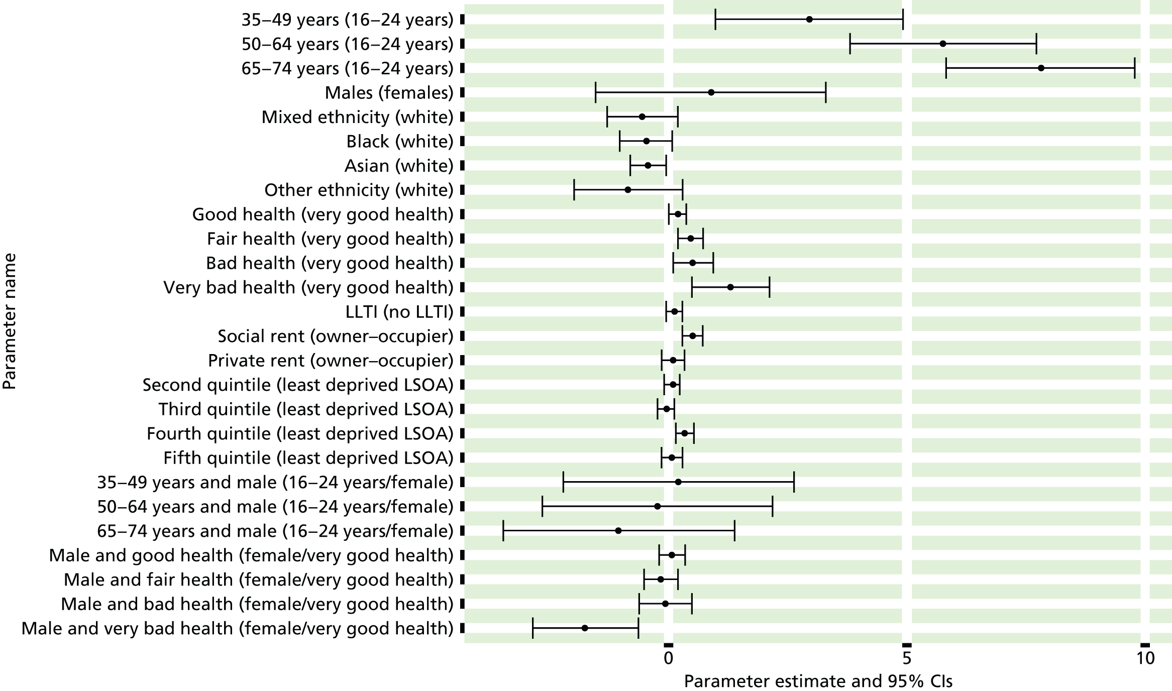
FIGURE 80.
Adults 25–74 years with ≥ 10% risk of CHD in next 10 years: individual estimates and their 95% CIs. (a) MSOAs; (b), LAs; (c) CCGs; and (d) regions (GORs).


Adults aged 25–74 years expected to develop coronary heart disease in the next 10 years (Health Survey for England, 2006 and 2009–11)
FIGURE 81.
Adults aged 25–74 years expected to develop CHD in next 10 years: LSOA-level map. Contains Ordnance Survey data © Crown copyright and database right 2012.
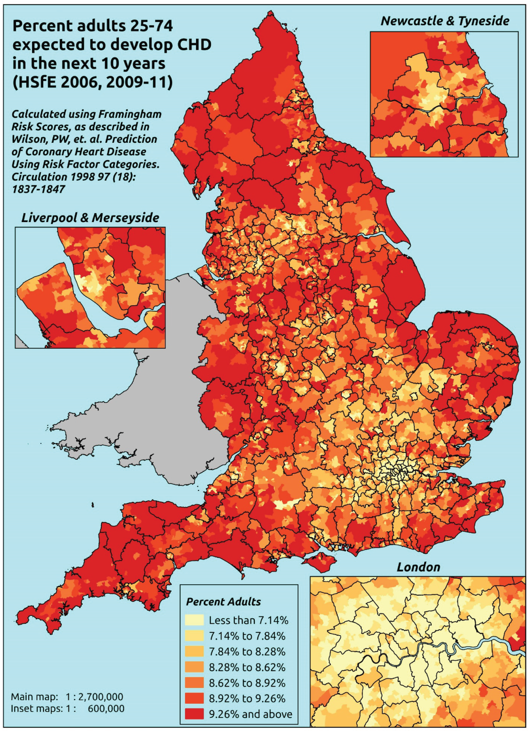
Response variable definition, provenance and prediction
Estimates of the proportion of adults aged 25–74 years likely to develop CHD in the next 10 years are based on HSfE data on respondents’ age, sex, cholesterol levels (total and high-density lipoprotein), blood pressure, whether or not they have diagnosed or undiagnosed diabetes and whether or not they smoke. Using the methodology described in Wilson et al. ,502 each respondent’s risk of developing CHD over the next 10 years is calculated. A generalised linear model (GLM) using the Gamma distribution and reciprocal link is used to model individuals’ estimated risk (as calculated using the Framingham Risk Calculator – see the previous section), using the usual set of sociodemographic predictor variables. (Note that the use of the reciprocal link means that a negative coefficient indicates that, relative to the reference group, a factor is associated with an increased risk of developing CHD in the next 10 years relative to the base.)
The HSfE at this time includes multiple household respondents of all ages. The analytical data set is drawn from the subset of respondents aged ≥ 16 years for whom data are available across all variables used to construct the individual risk score (namely their age and sex, nurse-administered blood tests of total and high-density lipoprotein cholesterol, blood pressure and glycated haemoglobin, smoking status and whether or not they have been diagnosed with diabetes – excluding in pregnancy), as well as the usual range of predictor variables, namely age, sex, ethnicity, general health status, LLTI and tenure, along with the IMD quintile of their LSOA of residence (n = 11,042). To avoid a household-level effect, a single randomly selected adult is drawn from each household, resulting in an analytical data set of 8176 adults aged ≥ 16 years.
The percentage of adults in each age–sex cohort, and overall, who are likely to develop CHD over the next 10 years are given in Table 103.
| Age band (years) | Females, % | Males, % | Overall, % |
|---|---|---|---|
| 25–34 | 2.5 | 3.3 | 2.9 |
| 35–49 | 4.2 | 5.7 | 4.8 |
| 50–64 | 9.8 | 11.9 | 10.7 |
| 65–74 | 17.0 | 17.2 | 17.1 |
| Total | 8.0 | 9.6 | 8.7 |
Model parameters (see below) are applied to microsimulated LSOA-level census data to produce estimates of the number (and proportion) of people to develop CHD in the next 10 years in each age–sex cohort (and overall) in each of the 32,844 English LSOAs. As discussed in the report, bootstrapping is used to derive 95% CIs for these estimates. The bootstrapped LSOA-level prevalence rate estimates are aggregated into a number of higher geographies, namely for MSOAs, LAs, CCGs, and regions (GORs), and are then used to calculate 95% CIs for these higher-level estimates. Proportionate attribution is used to restructure the estimates to align with 2001 MSOAs, as well as GP practice populations as defined by the 2011 NHS ADS.
Table 104 summarises how expected prevalence rates vary by age, sex and local deprivation (as measured by the 2010 IMD). There are 6569 LSOAs (with 9,226,227 adults) classified as being in the least deprived quintile; 6568 LSOAs (9,525,344 adults) in the second least deprived quintile; 6568 LSOAs (9,658,444 adults) in the third least deprived quintile; 6568 LSOAs (9,650,576 adults) in the fourth least deprived quintile; and 6568 LSOAs (9,535,167 adults) in the most deprived quintile. Note that, as a general rule, variations in prevalence rates reflect variations in the socioeconomic composition of populations in the different types of LSOA rather than variations in deprivation per se.
| Cohort | Least deprived quintile LSOAs | Second least deprived quintile LSOAs | Third least deprived quintile LSOAs | Fourth least deprived quintile LSOAs | Most deprived quintile LSOAs | All England |
|---|---|---|---|---|---|---|
| Female 25–34 | 2.4 (2.3 to 2.6) | 2.3 (2.2 to 2.4) | 2.4 (2.3 to 2.6) | 2.5 (2.4 to 2.7) | 2.7 (2.5 to 2.9) | 2.5 (2.4 to 2.6) |
| Female 35–49 | 3.8 (3.7 to 3.9) | 4.1 (3.9 to 4.2) | 4.1 (4.0 to 4.3) | 4.4 (4.3 to 4.6) | 4.4 (4.3 to 4.6) | 4.2 (4.1 to 4.3) |
| Female 50–64 | 9.4 (9.1 to 9.7) | 9.7 (9.4 to 10.1) | 9.6 (9.3 to 10.0) | 10.8 (10.4 to 11.2) | 10.9 (10.4 to 11.5) | 10.1 (9.8 to 10.3) |
| Female 65–74 | 16.2 (15.7 to 16.8) | 17.7 (16.9 to 18.5) | 17.1 (16.1 to 17.7) | 17.8 (16.5 to 18.7) | 19.3 (17.8 to 20.7) | 17.5 (16.9 to 17.9) |
| Females | 7.6 (7.4 to 7.9) | 8.0 (7.7 to 8.3) | 7.6 (7.3 to 7.9) | 7.7 (7.3 to 8.0) | 7.6 (7.2 to 8.0) | 7.7 (7.5 to 7.9) |
| Male 25–34 | 3.3 (3.1 to 3.5) | 3.0 (2.8 to 3.2) | 3.3 (3.1 to 3.5) | 3.4 (3.2 to 3.6) | 3.7 (3.3 to 4.2) | 3.4 (3.2 to 3.6) |
| Male 35–49 | 5.2 (5.0 to 5.4) | 5.6 (5.4 to 5.9) | 5.6 (5.4 to 5.9) | 6.2 (6.0 to 6.5) | 6.2 (5.9 to 6.4) | 5.8 (5.6 to 5.9) |
| Male 50–64 | 11.4 (10.9 to 11.8) | 11.8 (11.3 to 12.1) | 11.5 (11.0 to 12.0) | 13.1 (12.5 to 13.5) | 12.9 (12.2 to 13.6) | 12.1 (11.7 to 12.3) |
| Male 65–74 | 16.3 (15.5 to 17.2) | 17.6 (16.6 to 18.5) | 16.7 (15.8 to 17.5) | 17.2 (15.9 to 18.1) | 18.1 (16.9 to 19.3) | 17.1 (16.5 to 17.6) |
| Males | 8.9 (8.5 to 9.3) | 9.2 (8.8 to 9.6) | 8.7 (8.3 to 9.1) | 8.9 (8.4 to 9.3) | 8.7 (8.2 to 9.3) | 8.9 (8.6 to 9.1) |
| All 25–74 | 8.2 (8.1 to 8.4) | 8.6 (8.4 to 8.8) | 8.1 (8.0 to 8.3) | 8.3 (8.0 to 8.4) | 8.2 (7.9 to 8.4) | 8.3 (8.2 to 8.4) |
| Factor (reference group) | Model coefficients | 95% CI | ||
|---|---|---|---|---|
| Estimate | Standard error | 2.5% CI | 97.50% | |
| (Intercept) | 42.43664 | 1.27651 | 39.93469 | 44.9386 |
| Age (25–34 years) | ||||
| 35–49 years | –16.3875 | 1.31137 | –18.9578 | –13.8172 |
| 50–64 years | –30.5711 | 1.27462 | –33.0694 | –28.0728 |
| 65–74 years | –35.1407 | 1.27426 | –37.6383 | –32.6432 |
| Sex (females) | ||||
| Males | –10.62500 | 1.44116 | –13.4497 | –7.80034 |
| Ethnicity (white) | ||||
| Mixed | 0.06519 | 0.79287 | –1.48884 | 1.61923 |
| Black | 1.67579 | 0.66176 | 0.37875 | 2.97283 |
| Asian | 1.16825 | 0.46497 | 0.25692 | 2.07959 |
| Other | 2.11972 | 1.48992 | –0.80053 | 5.03997 |
| General health status (very good) | ||||
| Good health | –0.94419 | 0.23098 | –1.39691 | –0.49148 |
| Fair health | –1.90994 | 0.26855 | –2.43631 | –1.38357 |
| Bad health | –1.77176 | 0.41437 | –2.58392 | –0.95960 |
| Very bad health | –2.04808 | 0.64886 | –3.31985 | –0.77631 |
| LLTI (no LTTI) | ||||
| LLTI | 0.08039 | 2.24780 | –4.32529 | 4.48607 |
| Tenure (owner–occupier) | ||||
| Social rent | –7.37434 | 1.91231 | –11.1225 | –3.62622 |
| Private rent or other tenure | –0.65215 | 1.65535 | –3.89663 | 2.59233 |
| LSOA deprivation quintile (least deprived) | ||||
| Second quintile | –0.42068 | 0.18695 | –0.78711 | –0.05425 |
| Third quintile | –0.20248 | 0.19473 | –0.58416 | 0.17919 |
| Fourth quintile | –0.86152 | 0.20072 | –1.25492 | –0.46812 |
| Fifth quintile ( = most deprived quintile) | –0.82423 | 0.22733 | –1.26978 | –0.37867 |
| Interaction effects | ||||
| 35–49 years and male (16–24 years/female) | 3.56172 | 1.48737 | 0.64647 | 6.47697 |
| 50–64 years and male (16–24 years/female) | 8.39016 | 1.44303 | 5.56182 | 11.2185 |
| 65–74 years and male (16–24 years/female) | 10.07211 | 1.44325 | 7.24333 | 12.90089 |
| Male and good health (female/very good health) | 0.18957 | 0.32000 | –0.43763 | 0.81678 |
| Male and fair health (female/very good health) | 1.02045 | 0.36178 | 0.31136 | 1.72955 |
| Male and bad health (female/very good health) | 1.36557 | 0.54573 | 0.29594 | 2.43520 |
| Male and very bad health (female/very good health) | 2.73321 | 1.04701 | 0.68108 | 4.78534 |
| 35–49 years and LLTI (16–24 years/no LLTI) | –1.58657 | 2.30138 | –6.09727 | 2.92413 |
| 50–64 years and LLTI (16–24 years/no LLTI) | –0.63821 | 2.25603 | –5.06003 | 3.78361 |
| 65–74 years and LLTI (16–24 years/no LLTI) | 0.22012 | 2.25483 | –4.19935 | 4.63959 |
| 35–49 years and social rent (16–24 years/owner–occupier) | 4.08132 | 1.98790 | 0.18504 | 7.97760 |
| 50–64 years and social rent (16–24 years/owner–occupier) | 6.34544 | 1.92995 | 2.56273 | 10.12814 |
| 65–74 years and social rent (16–24 years/owner–occupier) | 7.01028 | 1.92927 | 3.22890 | 10.79166 |
| 35–49 years and private rent (16–24 years/owner–occupier) | 0.33550 | 1.78713 | –3.16727 | 3.83827 |
| 50–64 years and private rent (16–24 years/owner–occupier) | 0.08391 | 1.69901 | –3.24615 | 3.41396 |
| 65–74 years and private rent (16–24 years/owner–occupier) | 0.43177 | 1.70898 | –2.91784 | 3.78138 |
FIGURE 82.
Parameter plots: adults aged 25–74 years expected to develop CHD in next 10 years.

FIGURE 83.
Adults aged 25–74 years expected to develop CHD in next 10 years: individual estimates and their 95% CIs. (a) MSOAs; (b) LAs; (c) CCGs; and (d) regions (GORs).


Three or more of the five National Institute for Health and Care Excellence cardiovascular disease modifiable risk factors (Health Survey for England, 2006 and 2009–11)
FIGURE 84.
Three or more of the five NICE CVD modifiable risk factors: LSOA-level map. Contains Ordnance Survey data © Crown copyright and database right 2012.

Response variable definition, provenance and prediction
This response variable seeks to capture variations in the prevalence of modifiable factors known to increase the risk of developing CVD, as detailed in NICE’s commissioning guide on services for the prevention of cardiovascular disease. 504
Referring to the nine modifiable risk factors identified by the Interheart study,505 the guide focuses on five key factors for which reliable data in more generally available, namely:
-
abnormal lipids (cholesterol > 5.0 mmol/l)
-
smoking or tobacco use
-
obesity
-
high blood pressure (hypertension)
-
diabetes.
Health Survey for England data are used to establish whether or not respondents exhibit ≥ 3 of these modifiable risk factors, and a binomial GLM with logistic link is fitted to the usual set of predictor variables.
The HSfE at this time includes multiple household respondents of all ages. The analytical data set is drawn from the subset of respondents aged ≥ 16 years for whom data are available across all variables describing individuals’ modifiable risk factors (namely nurse-administered blood tests for total cholesterol and glycated haemoglobin, nurse-administered height, weight and blood pressure measurements, and questions on smoking status and whether or not they have been diagnosed with diabetes – excluding in pregnancy), as well as the usual range of predictor variables, namely age, sex, ethnicity, general health status, LLTI and tenure, along with the IMD quintile of their LSOA of residence (n = 13,452). To avoid a household-level effect, a single randomly selected adult is drawn from each household, resulting in an analytical data set of 9498 adults aged ≥ 16 years.
| Age band (years) | Females | Age band (years) | Males | ||||
|---|---|---|---|---|---|---|---|
| Does not have condition | Has condition | % | Does not have condition | Has condition | % | ||
| 16–24 | 299 | 10 | 3.2 | 16–24 | 226 | 7 | 3.0 |
| 25–34 | 673 | 37 | 5.2 | 25–34 | 504 | 42 | 7.7 |
| 35–49 | 1529 | 184 | 10.7 | 35–49 | 1054 | 184 | 14.9 |
| 50–64 | 1258 | 333 | 20.9 | 50–64 | 956 | 273 | 22.2 |
| 65–74 | 468 | 165 | 26.1 | 65–74 | 396 | 95 | 19.3 |
| 75–84 | 299 | 99 | 24.9 | 75–84 | 202 | 35 | 14.8 |
| ≥ 85 | 88 | 26 | 22.8 | ≥ 85 | 47 | 9 | 16.1 |
| Females | 4614 | 854 | 15.6 | Males | 3385 | 645 | 16.0 |
| Total (males and females) | 7999 | 1499 | 15.8 | ||||
Model parameters (see below) are applied to microsimulated LSOA-level census data to produce estimates of the number (and proportion) of people expected to exhibit at least three modifiable CVD risk factors in each age–sex cohort (and overall) in each of the 32,844 English LSOAs. As discussed in the report, bootstrapping is used to derive 95% CIs for these estimates. The bootstrapped LSOA-level prevalence rate estimates are aggregated into a number of higher geographies, namely for MSOAs, LAs, CCGs and regions (GORs), and are then used to calculate 95% CIs for these higher-level estimates. Proportionate attribution is used to restructure the estimates to align with 2001 MSOAs, as well as GP practice populations as defined by the 2011 NHS ADS.
Table 107 summarises how expected prevalence rates vary by age, sex and local deprivation (as measured by the 2010 IMD). There are 6569 LSOAs (with 9,226,227 adults) classified as being in the least deprived quintile; 6568 LSOAs (9,525,344 adults) in the second least deprived quintile; 6568 LSOAs (9,658,444 adults) in the third least deprived quintile; 6568 LSOAs (9,650,576 adults) in the fourth least deprived quintile; and 6568 LSOAs (9,535,167 adults) in the most deprived quintile. Note that, as a general rule, variations in prevalence rates reflect variations in the socioeconomic composition of populations in the different types of LSOA rather than variations in deprivation per se.
| Cohort | Least deprived quintile LSOAs | Second least deprived quintile LSOAs | Third least deprived quintile LSOAs | Fourth least deprived quintile LSOAs | Most deprived quintile LSOAs | All England |
|---|---|---|---|---|---|---|
| Female 16–24 | 2.0 (1.0 to 3.2) | 2.6 (1.5 to 4.2) | 2.5 (1.4 to 4.2) | 2.9 (1.6 to 4.9) | 3.2 (1.7 to 5.2) | 2.7 (1.5 to 4.4) |
| Female 25–34 | 3.4 (2.5 to 4.2) | 4.4 (3.3 to 5.4) | 4.3 (3.3 to 5.5) | 5.0 (3.8 to 6.4) | 5.6 (4.3 to 7.0) | 4.7 (3.6 to 5.9) |
| Female 35–49 | 8.3 (7.0 to 9.3) | 10.7 (9.2 to 12.0) | 10.5 (9.1 to 11.7) | 12.2 (10.6 to 13.8) | 13.8 (11.8 to 15.7) | 11.1 (9.8 to 12.1) |
| Female 50–64 | 18.0 (15.9 to 20.2) | 22.4 (20.5 to 25.0) | 22.1 (19.9 to 24.6) | 25.3 (23.3 to 28.4) | 28.1 (25.7 to 31.1) | 22.9 (21.4 to 25.0) |
| Female 65–74 | 22.0 (19.4 to 24.8) | 27.2 (24.4 to 30.5) | 26.8 (24.0 to 29.7) | 30.6 (27.4 to 33.9) | 33.7 (30.3 to 37.5) | 27.6 (25.1 to 30.2) |
| Female ≥ 75 | 20.6 (17.6 to 23.4) | 25.4 (22.2 to 29.0) | 24.9 (21.3 to 28.7) | 28.2 (25.3 to 32.2) | 30.6 (27.0 to 34.4) | 25.7 (23.1 to 29.0) |
| Females | 13.1 (11.2 to 14.9) | 16.2 (14.3 to 18.4) | 15.2 (13.3 to 17.3) | 16.2 (14.3 to 18.6) | 17.0 (14.8 to 19.4) | 15.5 (14.0 to 17.4) |
| Male 16–24 | 1.9 (0.8 to 3.0) | 2.5 (1.0 to 3.8) | 2.4 (1.0 to 3.7) | 2.7 (1.2 to 4.4) | 3.1 (1.3 to 5.0) | 2.6 (1.1 to 4.1) |
| Male 25–34 | 5.4 (4.1 to 6.7) | 6.9 (5.5 to 8.7) | 6.6 (5.3 to 8.3) | 7.6 (6.1 to 9.6) | 8.4 (6.6 to 10.3) | 7.2 (5.8 to 8.9) |
| Male 35–49 | 11.5 (9.9 to 12.9) | 14.6 (12.8 to 16.6) | 14.2 (12.3 to 16.2) | 16.2 (14.6 to 18.4) | 17.8 (15.7 to 19.9) | 14.9 (13.3 to 16.4) |
| Male 50–64 | 18.8 (16.5 to 20.7) | 23.3 (20.7 to 25.8) | 22.7 (20.2 to 25.0) | 25.7 (23.4 to 28.5) | 27.9 (25.1 to 30.9) | 23.5 (21.4 to 25.3) |
| Male 65–74 | 16.4 (13.2 to 18.8) | 20.3 (17.0 to 23.5) | 19.9 (16.7 to 23.0) | 22.6 (19.2 to 26.2) | 24.6 (20.7 to 28.5) | 20.4 (17.1 to 23.2) |
| Male ≥ 75 | 12.0 (9.2 to 15.0) | 15.0 (12.0 to 18.9) | 14.8 (11.4 to 18.6) | 16.8 (13.3 to 21.2) | 18.4 (14.7 to 22.7) | 15.1 (12.0 to 18.8) |
| Males | 12.3 (10.3 to 14.1) | 15.2 (12.9 to 17.5) | 14.2 (12.0 to 16.5) | 15.3 (13.2 to 17.8) | 16.2 (13.8 to 18.8) | 14.6 (12.7 to 16.6) |
| All | 12.7 (11.4 to 13.8) | 15.7 (14.5 to 16.9) | 14.7 (13.6 to 15.9) | 15.7 (14.7 to 17.1) | 16.6 (15.4 to 18.0) | 15.1 (14.6 to 15.8) |
| Factor (reference group) | Model coefficients | 95% CI | ||
|---|---|---|---|---|
| Estimate | Standard error | 2.5% CI | 97.50% | |
| (Intercept) | –4.16945 | 0.33441 | –4.8249 | –3.51401 |
| Age (16–24 years) | ||||
| 25–34 years | 0.55485 | 0.36449 | –0.15954 | 1.26924 |
| 35–49 years | 1.37677 | 0.33304 | 0.72400 | 2.02953 |
| 50–64 years | 2.12375 | 0.33041 | 1.47614 | 2.77137 |
| 65–74 years | 2.34346 | 0.33763 | 1.68171 | 3.00521 |
| 75–84 years | 2.17336 | 0.34596 | 1.49528 | 2.85144 |
| ≥ 85 years | 1.99120 | 0.39661 | 1.21384 | 2.76857 |
| Sex (females) | ||||
| Males | 0.01243 | 0.50217 | –0.97184 | 0.99669 |
| Ethnicity (white) | ||||
| Mixed | 0.02866 | 0.30972 | –0.57839 | 0.63571 |
| Black | –0.37634 | 0.24879 | –0.86397 | 0.11128 |
| Asian | –0.99713 | 0.23125 | –1.45039 | –0.54388 |
| Other | –0.79780 | 0.61246 | –1.99822 | 0.40262 |
| General health status (very good) | ||||
| Good health | 0.55171 | 0.07429 | 0.40610 | 0.69732 |
| Fair health | 0.72479 | 0.09666 | 0.53535 | 0.91424 |
| Bad health | 0.81735 | 0.14952 | 0.52430 | 1.11041 |
| Very bad health | 0.34447 | 0.28741 | –0.21885 | 0.90780 |
| LLTI (no LTTI) | ||||
| LLTI | 0.08647 | 0.09323 | –0.09627 | 0.26920 |
| Tenure (owner–occupier) | ||||
| Social rent | 0.35778 | 0.08693 | 0.18739 | 0.52817 |
| Private rent or other tenure | 0.17286 | 0.10512 | –0.03318 | 0.37891 |
| LSOA deprivation quintile (least deprived quintile) | ||||
| Second quintile | 0.24560 | 0.08991 | 0.06937 | 0.42183 |
| Third quintile | 0.19896 | 0.09230 | 0.01805 | 0.37987 |
| Fourth quintile | 0.33431 | 0.09465 | 0.14879 | 0.51983 |
| Fifth quintile ( = most deprived quintile) | 0.40264 | 0.10428 | 0.19825 | 0.60703 |
| Interaction effects | ||||
| 25–34 years and male (16–24 years/female) | 0.49595 | 0.55397 | –0.58983 | 1.58173 |
| 35–49 years and male (16–24 years/female) | 0.41993 | 0.51462 | –0.58872 | 1.42859 |
| 50–64 years and male (16–24 years/female) | 0.13090 | 0.51135 | –0.87135 | 1.13314 |
| 65–74 years and male (16–24 years/female) | –0.26994 | 0.52426 | –1.29749 | 0.75760 |
| 75–84 years and male (16–24 years/female) | –0.49224 | 0.54967 | –1.56960 | 0.58512 |
| ≥ 85 years and male (16–24 years/female) | –0.29679 | 0.66358 | –1.59741 | 1.00383 |
| Male and LLTI (female/no LLTI) | –0.29702 | 0.13369 | –0.55905 | –0.03499 |
FIGURE 85.
Parameter plots: three or more of the five NICE CVD modifiable risk factors.
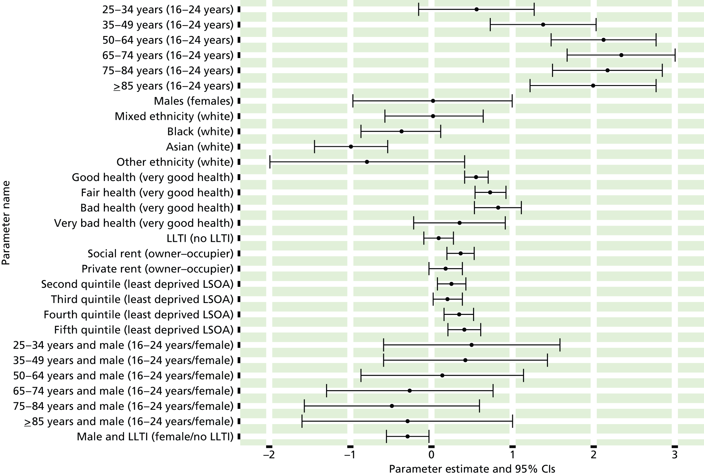
FIGURE 86.
Three or more of the five NICE CVD modifiable risk factors: individual estimates and their 95% CIs. (a) MSOAs; (b) LAs; (c) CCGs; and (d) regions (GORs).


Appendix 27 Mental health prevalence estimates
Clinical Interview Schedule – Revised score of ≥ 12 (Adult Psychiatry Morbidity Survey, 2007)
FIGURE 87.
Clinical Interview Schedule – Revised score of ≥ 12: LSOA-level map. Contains Ordnance Survey data © Crown copyright and database right 2012.
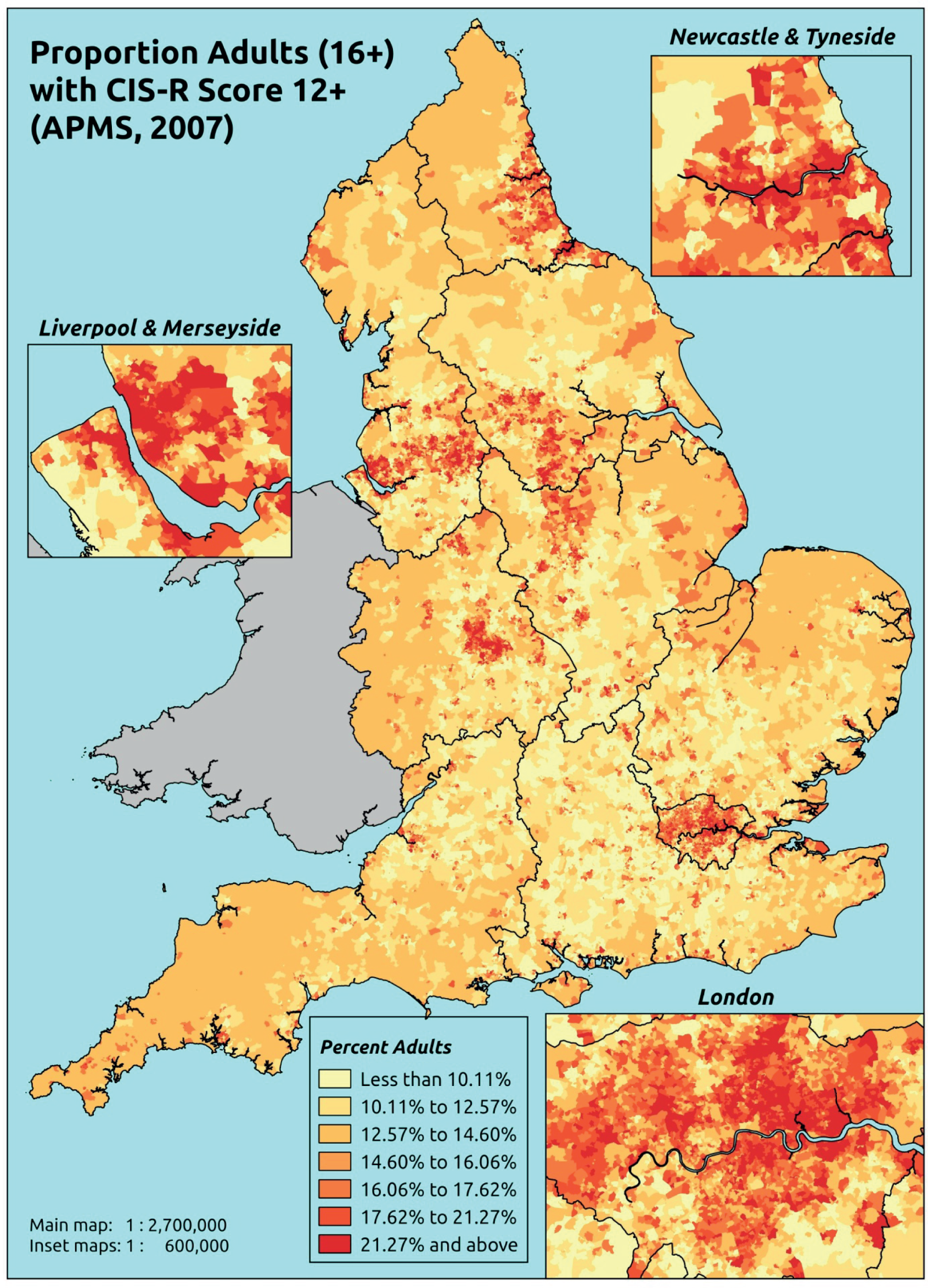
Response variable definition, provenance and prediction
Derived from the CIS-R, a score of ≥ 12 is widely taken as being indicative of the presence of a common mental disorder. Here we estimate the proportion of people in each age–sex cohort, and overall, for adults aged ≥ 16 years, with a CIS-R score of ≥ 12. Although this marker of need is based on a well-established instrument incorporated within the APMS, it is not independent of sociodemographic or geographic variations in access to, or uptake of, care, as individuals may score < 12 precisely because they are being treated for a mental health problem (see the alternative marker below which includes people currently being treated).
The APMS data set (n = 7403) comprises adults aged ≥ 16 years (living in England) and surveyed only one person per household; thus, the analytical data set contains all respondents for whom data is available across all model response and predictor variables, namely CIS-R score, age band, sex, ethnicity, LLTI, tenure and IMD quintile of LSOA of residence (n = 7326).
| Age band (years) | Females | Age band (years) | Males | ||||
|---|---|---|---|---|---|---|---|
| Does not have condition | Has condition | % | Does not have condition | Has condition | % | ||
| 16–24 | 225 | 68 | 23.2 | 16–24 | 233 | 33 | 12.4 |
| 25–34 | 476 | 138 | 22.5 | 25–34 | 347 | 60 | 14.7 |
| 35–49 | 866 | 250 | 22.4 | 35–49 | 744 | 127 | 14.6 |
| 50–64 | 822 | 191 | 18.9 | 50–64 | 694 | 103 | 12.9 |
| 65–74 | 487 | 75 | 13.3 | 65–74 | 428 | 33 | 7.2 |
| 75–84 | 386 | 49 | 11.3 | 75–84 | 268 | 18 | 6.3 |
| ≥ 85 | 122 | 11 | 8.3 | ≥ 85 | 68 | 4 | 5.6 |
| Females | 3384 | 782 | 18.8 | Males | 2782 | 378 | 12.0 |
| Total (males and females) | 6166 | 1160 | 15.8 | ||||
Model parameters are applied to microsimulated LSOA-level census data to produce estimates of the number (and proportion) of people expected to return a CIS-R score of ≥ 12 in each age–sex cohort (and overall) in each of the 32,844 English LSOAs. As discussed in the report, bootstrapping is used to derive 95% CIs for the estimates. These LSOA-level prevalence rate estimates (and 95% CIs) are aggregated into a number of higher geographies, namely MSOAs, LAs, CCGs and regions (GORs). Proportionate attribution is used to restructure the prevalence rate estimates to align with 2001 MSOAs, as well as GP practice populations as defined by the 2011 NHS ADS.
Table 110 summarises how expected prevalence rates vary by age, sex and local deprivation (as measured by the 2010 IMD). There are 6569 LSOAs (with 9,226,227 adults) classified as being in the least deprived quintile; 6568 LSOAs (9,525,344 adults) in the second least deprived quintile; 6568 LSOAs (9,658,444 adults) in the third least deprived quintile; 6568 LSOAs (9,650,576 adults) in the fourth least deprived quintile; and 6568 LSOAs (9,535,167 adults) in the most deprived quintile. Note that, as a general rule, variations in prevalence rates reflect variations in the socioeconomic composition of populations in the different types of LSOA rather than variations in deprivation per se.
| Cohort | Least deprived quintile LSOAs | Second least deprived quintile LSOAs | Third least deprived quintile LSOAs | Fourth least deprived quintile LSOAs | Most deprived quintile LSOAs | All England |
|---|---|---|---|---|---|---|
| Female 16–24 | 17.0 (13.0 to 22.3) | 19.0 (16.2 to 24.7) | 23.9 (20.0 to 29.5) | 19.3 (15.5 to 23.5) | 23.5 (21.3 to 30.1) | 20.9 (18.5 to 25.3) |
| Female 25–34 | 14.4 (12.3 to 18.2) | 16.9 (15.3 to 21.4) | 22.2 (19.4 to 26.4) | 19.7 (16.6 to 22.9) | 25.8 (23.7 to 31.2) | 20.6 (18.6 to 23.9) |
| Female 35–49 | 14.6 (11.8 to 16.8) | 18.0 (15.8 to 20.4) | 23.9 (20.5 to 25.7) | 23.2 (19.7 to 25.1) | 30.3 (27.6 to 33.8) | 22.0 (19.7 to 23.5) |
| Female 50–64 | 11.7 (10.2 to 14.5) | 16.0 (14.5 to 18.5) | 20.7 (18.5 to 23.7) | 22.5 (19.3 to 25.6) | 29.5 (27.0 to 34.3) | 19.6 (18.1 to 22.1) |
| Female 65–74 | 7.5 (5.8 to 9.4) | 11.3 (9.1 to 13.7) | 14.1 (11.4 to 17.2) | 16.3 (12.3 to 19.6) | 20.1 (16.3 to 25.1) | 13.4 (11.2 to 15.8) |
| Female ≥ 75 | 7.1 (5.4 to 9.9) | 11.1 (8.3 to 13.5) | 12.5 (9.6 to 15.5) | 13.6 (10.0 to 17.6) | 14.5 (11.2 to 18.9) | 11.6 (9.3 to 14.4) |
| Females | 12.1 (9.9 to 15.0) | 15.6 (13.5 to 18.7) | 20.2 (17.2 o 23.4) | 20.0 (16.6 to 23.1) | 25.6 (22.9 to 30.4) | 18.7 (16.7 to 21.4) |
| Male 16–24 | 10.1 (7.3 to 13.6) | 11.8 (9.5 to 15.5) | 15.3 (12.1 to 18.6) | 12.9 (10.0 to 15.7) | 16.6 (14.8 to 20.9) | 13.6 (11.6 to 16.5) |
| Male 25–34 | 8.5 (6.8 to 10.9) | 10.5 (9.0 to 13.3) | 14.2 (11.9 to 17.0) | 13.1 (10.6 to 15.2) | 18.6 (16.2 to 22.5) | 13.6 (11.9 to 15.9) |
| Male 35–49 | 8.5 (6.2 to 9.7) | 10.9 (8.8 to 12.3) | 15.0 (11.9 to 16.4) | 15.3 (12.6 to 16.2) | 21.7 (19.0 to 23.8) | 14.3 (12.2 to 15.1) |
| Male 50–64 | 6.6 (5.3 to 8.1) | 9.4 (8.0 to 11.2) | 12.7 (10.9 to 14.7) | 14.6 (11.9 to 16.5) | 20.3 (17.6 to 23.8) | 12.4 (10.9 to 14.0) |
| Male 65–74 | 4.1 (3.0 to 5.1) | 6.6 (4.9 to 8.0) | 8.4 (6.5 to 10.5) | 10.1 (7.4 to 11.9) | 13.2 (10.4 to 16.6) | 8.1 (6.5 to 9.6) |
| Male ≥ 75 | 3.9 (2.8 to 5.5) | 6.2 (4.2 to 7.7) | 7.3 (5.2 to 9.2) | 8.2 (5.8 to 10.5) | 9.3 (6.8 to 12.6) | 6.7 (5.2 to 8.5) |
| Males | 7.1 (5.4 to 8.8) | 9.5 (7.7 to 11.5) | 12.8 (10.4 to 14.9) | 13.2 (10.6 to 15.1) | 18.3 (15.8 to 21.6) | 12.2 (10.4 to 13.9) |
| All | 9.7 (8.4 to 11.3) | 12.7 (11.6 to 14.1) | 16.6 (14.9 to 18.2) | 16.7 (14.5 to 18.3) | 22.0 (20.9 to 24.7) | 15.6 (14.9 to 16.5) |
| Factor (reference group) | Model coefficients | 95% CI | ||
|---|---|---|---|---|
| Estimate | SE | 2.5% CI | 97.5% | |
| (Intercept) | –1.69971 | 0.21664 | –2.12432 | –1.2751 |
| Age (16–24 years) | ||||
| 25–34 years | –0.44013 | 0.22313 | –0.87747 | –0.00279 |
| 35–49 years | –0.44214 | 0.19884 | –0.83186 | –0.05241 |
| 50–64 years | –0.82381 | 0.20275 | –1.22121 | –0.42641 |
| 65–74 years | –1.54817 | 0.22996 | –1.99889 | –1.09745 |
| 75–84 years | –1.76752 | 0.2474 | –2.25241 | –1.28262 |
| ≥ 85 years | –1.96847 | 0.36421 | –2.68233 | –1.25461 |
| Sex (females) | ||||
| Males | –0.65139 | 0.09587 | –0.83929 | –0.46349 |
| Ethnicity (white) | ||||
| Mixed | 0.18437 | 0.40067 | –0.60094 | 0.96969 |
| Black | –0.43721 | 0.27113 | –0.96864 | 0.09421 |
| Asian | –0.13946 | 0.26787 | –0.66449 | 0.38556 |
| Other | 0.65314 | 0.44709 | –0.22316 | 1.52943 |
| LLTI (no LTTI) | ||||
| LLTI | 1.26179 | 0.19524 | 0.87912 | 1.64445 |
| Tenure (owner–occupier) | ||||
| Social rent | 0.16883 | 0.28047 | –0.38089 | 0.71855 |
| Private rent or other tenure | –0.20441 | 0.30836 | –0.80879 | 0.39996 |
| LSOA deprivation quintile (least deprived quintile) | ||||
| Second LSOA deprivation quintile | 0.06721 | 0.16205 | –0.25041 | 0.38483 |
| Third LSOA deprivation quintile | 0.40613 | 0.15910 | 0.09429 | 0.71796 |
| Fourth LSOA deprivation quintile | 0.02185 | 0.16936 | –0.31010 | 0.35380 |
| Fifth LSOA deprivation quintile ( = most deprived) | 0.27737 | 0.16442 | –0.04489 | 0.59963 |
| Interaction effects | ||||
| Male and social rent | 0.41371 | 0.17039 | 0.07974 | 0.74767 |
| Male and private rent or other tenure | –0.10108 | 0.22725 | –0.54648 | 0.34433 |
| Mixed and LLTI | 0.53643 | 0.77155 | –0.97582 | 2.04867 |
| Black and LLTI | 1.24709 | 0.40753 | 0.44834 | 2.04584 |
| Asian and LLTI | –0.09489 | 0.41381 | –0.90596 | 0.71618 |
| Other and LLTI | –0.20076 | 0.79171 | –1.75252 | 1.35100 |
| LLTI and second deprivation quintile | 0.45842 | 0.24981 | –0.03120 | 0.94804 |
| LLTI and third deprivation quintile | 0.24101 | 0.24399 | –0.23722 | 0.71924 |
| LLTI and fourth deprivation quintile | 0.74420 | 0.24951 | 0.25517 | 1.23323 |
| LLTI and fifth deprivation quintile | 0.53660 | 0.24008 | 0.06604 | 1.00716 |
| 25–34 years and social rent | 0.83346 | 0.34185 | 0.16344 | 1.50348 |
| 35–49 years and social rent | 0.56488 | 0.30980 | –0.04232 | 1.17209 |
| 50–64 years and social rent | 0.37222 | 0.31758 | –0.25024 | 0.99469 |
| 65–74 years and social rent | 0.18544 | 0.35905 | –0.51830 | 0.88918 |
| 75–84 years and social rent | –0.43845 | 0.40902 | –1.24012 | 0.36322 |
| ≥ 85 years and social rent | –1.10881 | 0.72522 | –2.53024 | 0.31262 |
| 25–34 years and private rent or other tenure | 0.77959 | 0.36797 | 0.05837 | 1.50082 |
| 35–49 years and private rent or other tenure | 0.81082 | 0.35437 | 0.11626 | 1.50539 |
| 50–64 years and private rent or other tenure | 0.45249 | 0.41387 | –0.35869 | 1.26367 |
| 65–74 years and private rent or other tenure | 0.17127 | 0.58864 | –0.98247 | 1.32500 |
| 75–84 years and private rent or other tenure | 0.09246 | 0.71221 | –1.30347 | 1.48839 |
| ≥ 85 years and private rent or other tenure | –11.76647 | 230.12616 | –462.814 | 439.2808 |
FIGURE 88.
Parameter plots: CIS-R score of ≥ 12.
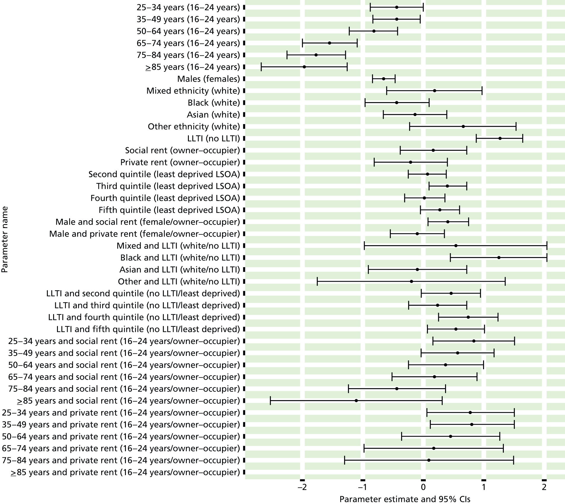
FIGURE 89.
Clinical Interview Schedule – Revised score of ≥ 12: individual estimates and their 95% CIs. (a) MSOAs; (b) LAs; (c) CCGs; and (d) regions (GORs).
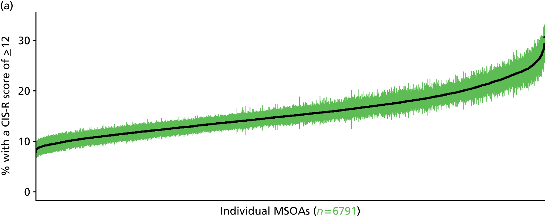

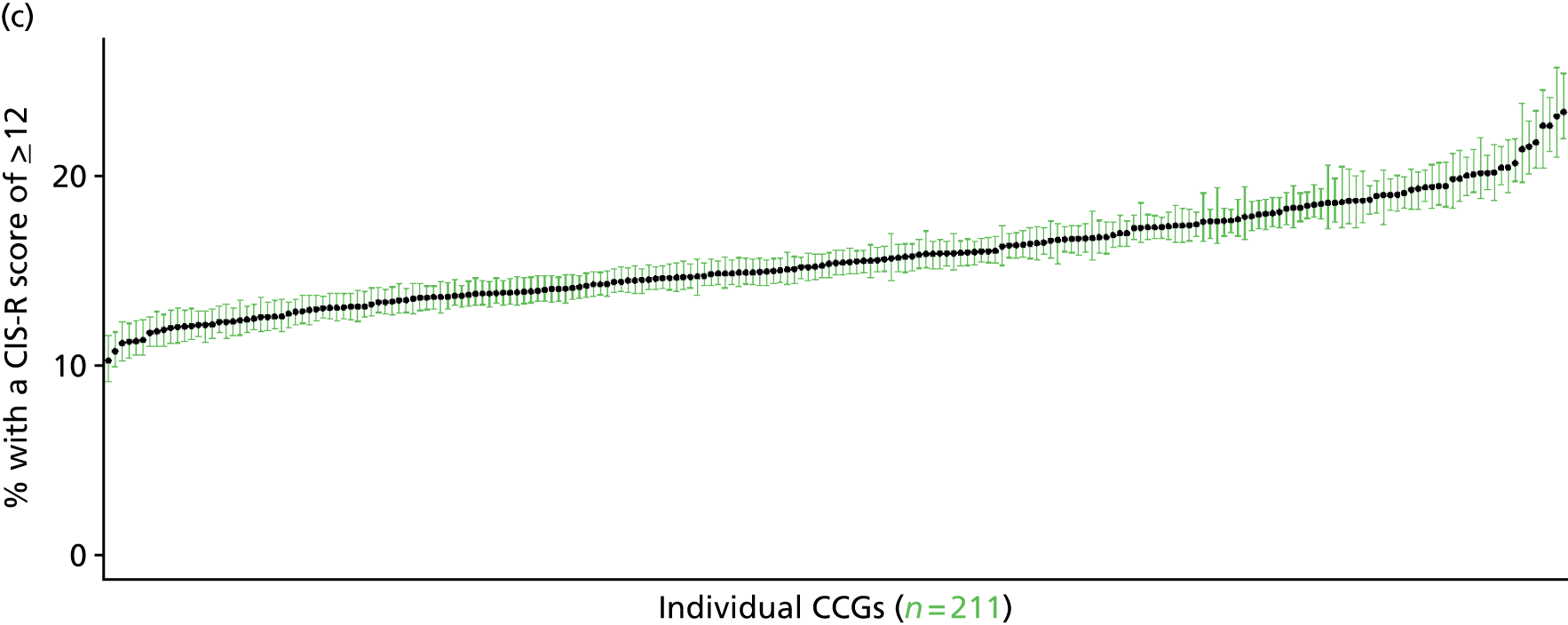

Clinical Interview Schedule – Revised score of ≥ 18 (Adult Psychiatry Morbidity Survey, 2007)
FIGURE 90.
Clinical Interview Schedule – Revised score of ≥ 18: LSOA-level map. Contains Ordnance Survey data © Crown copyright and database right 2012.
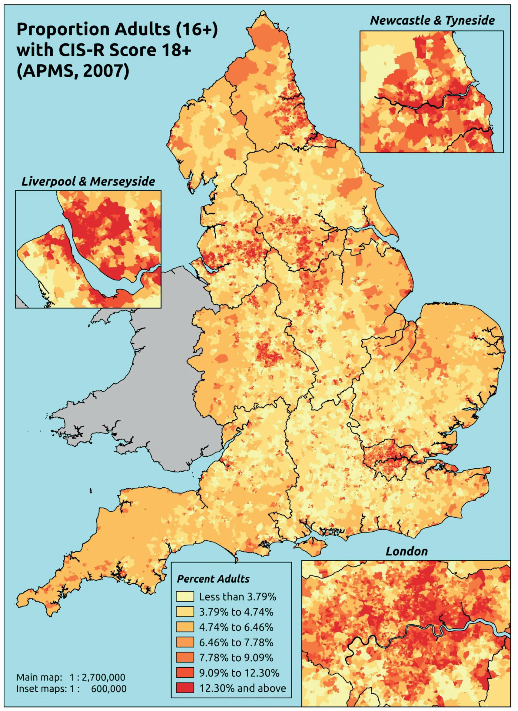
Response variable definition, provenance and prediction
Derived from CIS-R, a score of ≥ 18 is widely taken as being indicative of the presence of a common mental disorder which requires treatment. Here we estimate the proportion of people in each age–sex cohort, and overall, for adults aged ≥ 16 years, with a CIS-R score of ≥ 18. Although this marker of need is based on a well-established instrument incorporated within the APMS, it is not independent of sociodemographic or geographic variations in access to, or uptake of, care, as individuals may score < 18 precisely because they are being treated for a mental health problem (see the alternative marker below which includes people currently being treated).
The APMS data set (n = 7403) comprises adults aged ≥ 16 years (living in England) and surveyed only one person per household; thus, the analytical data set contains all respondents for whom data are available across all model response and predictor variables, namely CIS-R score, age band, sex, ethnicity, LLTI, tenure and IMD quintile of LSOA of residence (n = 7326).
| Age band (years) | Females | Age band (years) | Males | ||||
|---|---|---|---|---|---|---|---|
| Does not have condition | Has condition | % | Does not have condition | Has condition | % | ||
| 16–24 | 252 | 41 | 14.0 | 16–24 | 249 | 17 | 6.4 |
| 25–34 | 548 | 66 | 10.7 | 25–34 | 375 | 32 | 7.9 |
| 35–49 | 980 | 136 | 12.2 | 35–49 | 805 | 66 | 7.6 |
| 50–64 | 912 | 101 | 10.0 | 50–64 | 739 | 58 | 7.3 |
| 65–74 | 534 | 28 | 5.0 | 65–74 | 453 | 8 | 1.7 |
| 75–84 | 417 | 18 | 4.1 | 75–84 | 279 | 7 | 2.4 |
| ≥ 85 | 129 | 4 | 3.0 | ≥ 85 | 70 | 2 | 2.8 |
| Females | 3772 | 394 | 9.5 | Males | 2970 | 190 | 6.0 |
| Total (males and females) | 6742 | 584 | 8.0 | ||||
Model parameters are applied to microsimulated LSOA-level census data to produce estimates of the number (and proportion) of people expected to return a CIS-R score of ≥ 18 in each age–sex cohort (and overall) in each of the 32,844 English LSOAs. As discussed in the report, bootstrapping is used to derive 95% CIs for the estimates. These LSOA-level prevalence rate estimates (and 95% CIs) are aggregated into a number of higher geographies, namely MSOAs, LAs, CCGs, and regions (GORs). Proportionate attribution is used to restructure the prevalence rate estimates to align with 2001 MSOAs, as well as GP practice populations as defined by the 2011 NHS ADS.
Table 113 summarises how expected prevalence rates vary by age, sex and local deprivation (as measured by the 2010 IMD). There are 6569 LSOAs (with 9,226,227 adults) classified as being in the least deprived quintile; 6568 LSOAs (9,525,344 adults) in the second least deprived quintile; 6568 LSOAs (9,658,444 adults) in the third least deprived quintile; 6568 LSOAs (9,650,576 adults) in the fourth least deprived quintile; and 6568 LSOAs (9,535,167 adults) in the most deprived quintile. Note that, as a general rule, variations in prevalence rates reflect variations in the socioeconomic composition of populations in the different types of LSOA rather than variations in deprivation per se.
| Cohort | Least deprived quintile LSOAs | Second least deprived quintile LSOAs | Third least deprived quintile LSOAs | Fourth least deprived quintile LSOAs | Most deprived quintile LSOAs | All England |
|---|---|---|---|---|---|---|
| Female 16–24 | 7.1 (4.4 to 11.3) | 8.4 (6.1 to 12.5) | 12.4 (9.1 to 17.4) | 11.3 (8.6 to 15.1) | 15.3 (12.8 to 20.2) | 11.4 (9.1 to 15.4) |
| Female 25–34 | 4.6 (3.4 to 6.3) | 6.0 (4.6 to 8.4) | 10.4 (8.4 to 13.4) | 9.2 (6.5 to 11.5) | 14.3 (12.1 to 18.3) | 9.5 (8.2 to 11.7) |
| Female 35–49 | 5.6 (4.0 to 6.9) | 7.5 (5.3 to 8.9) | 12.5 (9.7 to 14.2) | 12.6 (9.9 to 14.4) | 19.7 (17.0 to 22.7) | 11.5 (9.8 to 12.7) |
| Female 50–64 | 5.0 (3.7 to 6.5) | 6.6 (5.4 to 8.3) | 11.1 (9.4 to 14.0) | 12.1 (9.5 to 14.8) | 19.4 (16.7 to 23.4) | 10.4 (9.2 to 12.2) |
| Female 65–74 | 2.1 (1.1 to 2.8) | 2.6 (1.6 to 3.7) | 4.8 (2.8 to 6.6) | 5.0 (3.0 to 6.6) | 8.2 (5.6 to 10.8) | 4.3 (2.8 to 5.5) |
| Female ≥ 75 | 3.1 (2.1 to 4.6) | 4.3 (2.8 to 6.4) | 6.4 (3.9 to 9.3) | 5.5 (3.7 to 7.9) | 7.8 (5.3 to 11.8) | 5.3 (3.7 to 7.7) |
| Females | 4.7 (3.3 to 6.3) | 6.1 (4.5 to 8.0) | 10.1 (7.7 to 12.8) | 10.0 (7.6 to 12.5) | 15.6 (13.0 to 19.3) | 9.3 (7.7 to 11.3) |
| Male 16–24 | 4.3 (2.5 to 6.5) | 5.0 (3.3 to 7.2) | 7.7 (5.4 to 10.0) | 7.5 (5.3 to 9.7) | 10.4 (8.1 to 13.5) | 7.3 (5.4 to 9.3) |
| Male 25–34 | 2.8 (1.8 to 3.6) | 3.4 (2.4 to 4.7) | 6.3 (4.8 to 8.4) | 5.8 (3.9 to 7.2) | 9.5 (7.4 to 12.1) | 6.0 (4.7 to 7.4) |
| Male 35–49 | 3.2 (2.1 to 3.7) | 4.1 (2.8 to 5.0) | 7.5 (5.5 to 8.8) | 7.9 (5.8 to 9.1) | 13.3 (10.6 to 15.5) | 7.2 (5.7 to 7.9) |
| Male 50–64 | 2.9 (1.9 to 3.5) | 3.7 (2.8 to 4.7) | 6.6 (5.0 to 8.4) | 7.7 (5.6 to 9.4) | 12.9 (10.0 to 15.4) | 6.5 (5.2 to 7.5) |
| Male 65–74 | 1.2 (0.6 to 1.5) | 1.5 (0.8 to 2.0) | 2.8 (1.6 to 3.7) | 3.2 (1.9 to 4.0) | 5.2 (3.3 to 6.8) | 2.6 (1.7 to 3.1) |
| Male ≥ 75 | 1.6 (1.1 to 2.4) | 2.2 (1.4 to 3.4) | 3.5 (2.1 to 5.5) | 3.0 (2.0 to 4.6) | 4.5 (2.8 to 7.4) | 2.9 (1.9 to 4.1) |
| Males | 2.7 (1.7 to 3.5) | 3.4 (2.4 to 4.6) | 6.1 (4.4 to 7.8) | 6.5 (4.6 to 8.0) | 10.6 (8.2 to 13.1) | 5.9 (4.5 to 7.0) |
| All | 3.7 (2.8 to 4.4) | 4.8 (3.8 to 5.8) | 8.2 (6.9 to 9.6) | 8.3 (6.7 to 9.6) | 13.1 (11.7 to 14.9) | 7.7 (7.0 to 8.3) |
| Factor (reference group) | Model coefficients | 95% CI | ||
|---|---|---|---|---|
| Estimate | SE | 2.5% CI | 97.5% | |
| (Intercept) | –2.84741 | 0.29913 | –3.43371 | –2.26111 |
| Age (16–24 years) | ||||
| 25–34 years | –0.79571 | 0.3157 | –1.41448 | –0.17693 |
| 35–49 years | –0.61097 | 0.26975 | –1.13968 | –0.08225 |
| 50–64 years | –1.01588 | 0.27528 | –1.55543 | –0.47633 |
| 65–74 years | –2.38890 | 0.35931 | –3.09314 | –1.68466 |
| 75–84 years | –2.19187 | 0.35704 | –2.89166 | –1.49208 |
| ≥ 85 years | –2.04559 | 0.49507 | –3.01594 | –1.07525 |
| Sex (females) | ||||
| Males | –0.62213 | 0.14293 | –0.90227 | –0.34199 |
| Ethnicity (white) | ||||
| Mixed | –0.60185 | 0.73575 | –2.04392 | 0.84023 |
| Black | –0.79344 | 0.46472 | –1.70428 | 0.11740 |
| Asian | –0.00007 | 0.34583 | –0.67790 | 0.67776 |
| Other | –0.02310 | 0.75084 | –1.49474 | 1.44854 |
| LTI (no LTTI) | ||||
| LLTI | 1.86324 | 0.10955 | 1.64852 | 2.07795 |
| Tenure (owner–occupier) | ||||
| Social rent | 0.78579 | 0.52779 | –0.24868 | 1.82026 |
| Private rent or other tenure | –0.79959 | 0.68153 | –2.13540 | 0.53621 |
| LSOA deprivation quintile (least deprived quintile) | ||||
| Second LSOA deprivation quintile | 0.24104 | 0.22096 | –0.19205 | 0.67412 |
| Third LSOA deprivation quintile | 0.46692 | 0.21956 | 0.03657 | 0.89727 |
| Fourth LSOA deprivation quintile | 0.60060 | 0.22188 | 0.16570 | 1.03549 |
| Fifth LSOA deprivation quintile ( = most deprived) | 0.91083 | 0.22431 | 0.47117 | 1.35049 |
| Interaction effects | ||||
| 25–34 years and social rent | 0.81569 | 0.43463 | –0.03619 | 1.66756 |
| 35–49 years and social rent | 0.58055 | 0.38270 | –0.16954 | 1.33063 |
| 50–64 years and social rent | 0.60057 | 0.38917 | –0.16220 | 1.36333 |
| 65–74 years and social rent | 0.69360 | 0.49418 | –0.27500 | 1.66219 |
| 75–84 years and social rent | –0.79932 | 0.62108 | –2.01665 | 0.41800 |
| ≥ 85 years and social rent | –14.0701 | 297.86920 | –597.89400 | 569.75350 |
| 25–34 years and private rent or other tenure | 1.14771 | 0.50517 | 0.15758 | 2.13784 |
| 35–49 years and private rent or other tenure | 0.92090 | 0.47841 | –0.01677 | 1.85858 |
| 50–64 years and private rent or other tenure | 0.52906 | 0.55074 | –0.55040 | 1.60852 |
| 65–74 years and private rent or other tenure | 0.64356 | 0.88014 | –1.08152 | 2.36865 |
| 75–84 years and private rent or other tenure | 1.20243 | 0.79194 | –0.34979 | 2.75464 |
| ≥ 85 years and private rent or other tenure | –12.9688 | 619.56110 | –1227.3100 | 1201.3710 |
| Male and social rent | 0.3899 | 0.21773 | –0.03685 | 0.81665 |
| Male and private rent or other tenure | –0.23958 | 0.31263 | –0.85233 | 0.37317 |
| Social rent and second LSOA deprivation quintile | –0.92318 | 0.54817 | –1.99759 | 0.15123 |
| Private rent or other tenure and second quintile | 0.63745 | 0.65310 | –0.64261 | 1.91752 |
| Social rent and third LSOA deprivation quintile | –0.24388 | 0.47012 | –1.16532 | 0.67755 |
| Private rent or other tenure and third quintile | 1.26042 | 0.61021 | 0.06440 | 2.45643 |
| Social rent and fourth LSOA deprivation quintile | –0.39366 | 0.45321 | –1.28196 | 0.49463 |
| Private rent or other tenure and fourth quintile | –0.10043 | 0.66037 | –1.39475 | 1.19389 |
| Social rent and fifth LSOA deprivation quintile | –0.72511 | 0.43906 | –1.58567 | 0.13544 |
| Private rent or other tenure and fifth quintile | 0.57724 | 0.61818 | –0.63439 | 1.78887 |
| Mixed and LLTI | 2.2230 | 1.00266 | 0.25778 | 4.18822 |
| Black and LLTI | 1.07645 | 0.57732 | –0.05510 | 2.20800 |
| Asian and LLTI | 0.03293 | 0.47853 | –0.90499 | 0.97086 |
| Other and LLTI | –0.20244 | 1.11174 | –2.38145 | 1.97657 |
FIGURE 91.
Parameter plots: CIS-R score of ≥ 18.
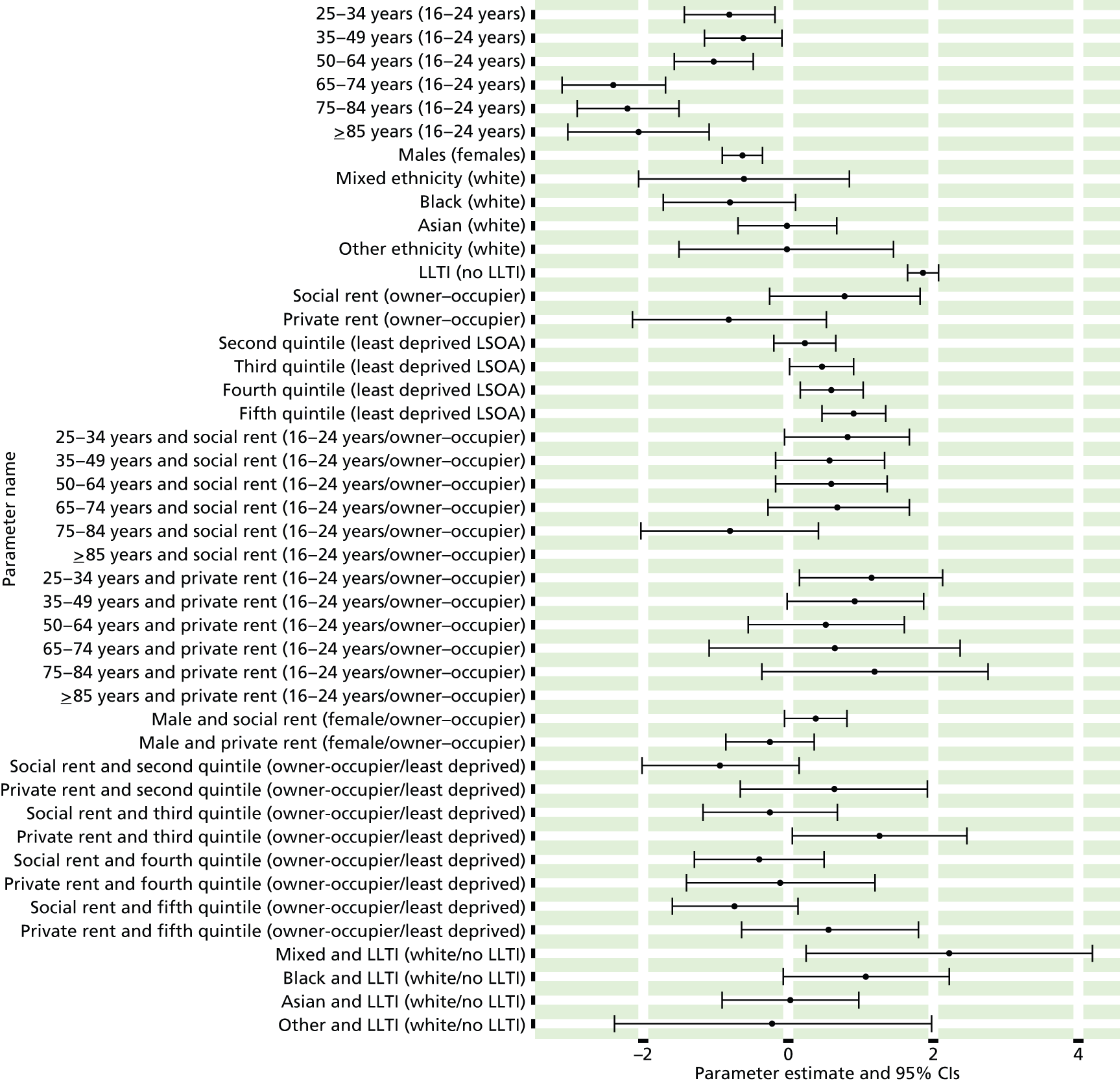
FIGURE 92.
Clinical Interview Schedule – Revised score of ≥ 18: individual estimates and their 95% CIs. (a) MSOAs; (b) LAs; (c) CCGs; and (d) regions (GORs).
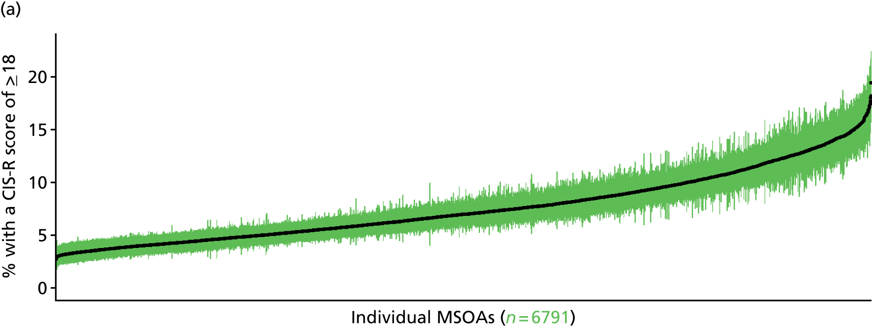
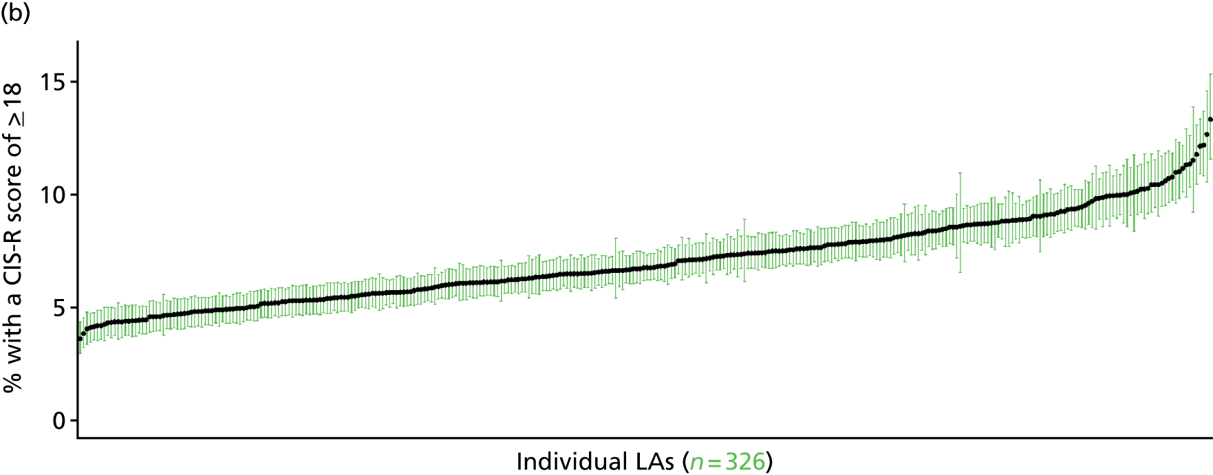
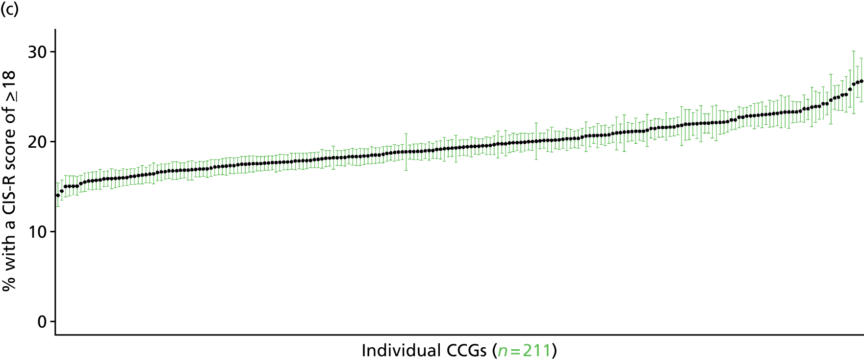
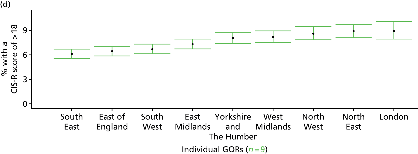
Clinical Interview Schedule – Revised score of ≥ 12 or any mental health treatment (Adult Psychiatry Morbidity Survey, 2007)
FIGURE 93.
Clinical Interview Schedule – Revised score of ≥ 12 or any mental health treatment: LSOA-level map. Contains Ordnance Survey data © Crown copyright and database right 2012.
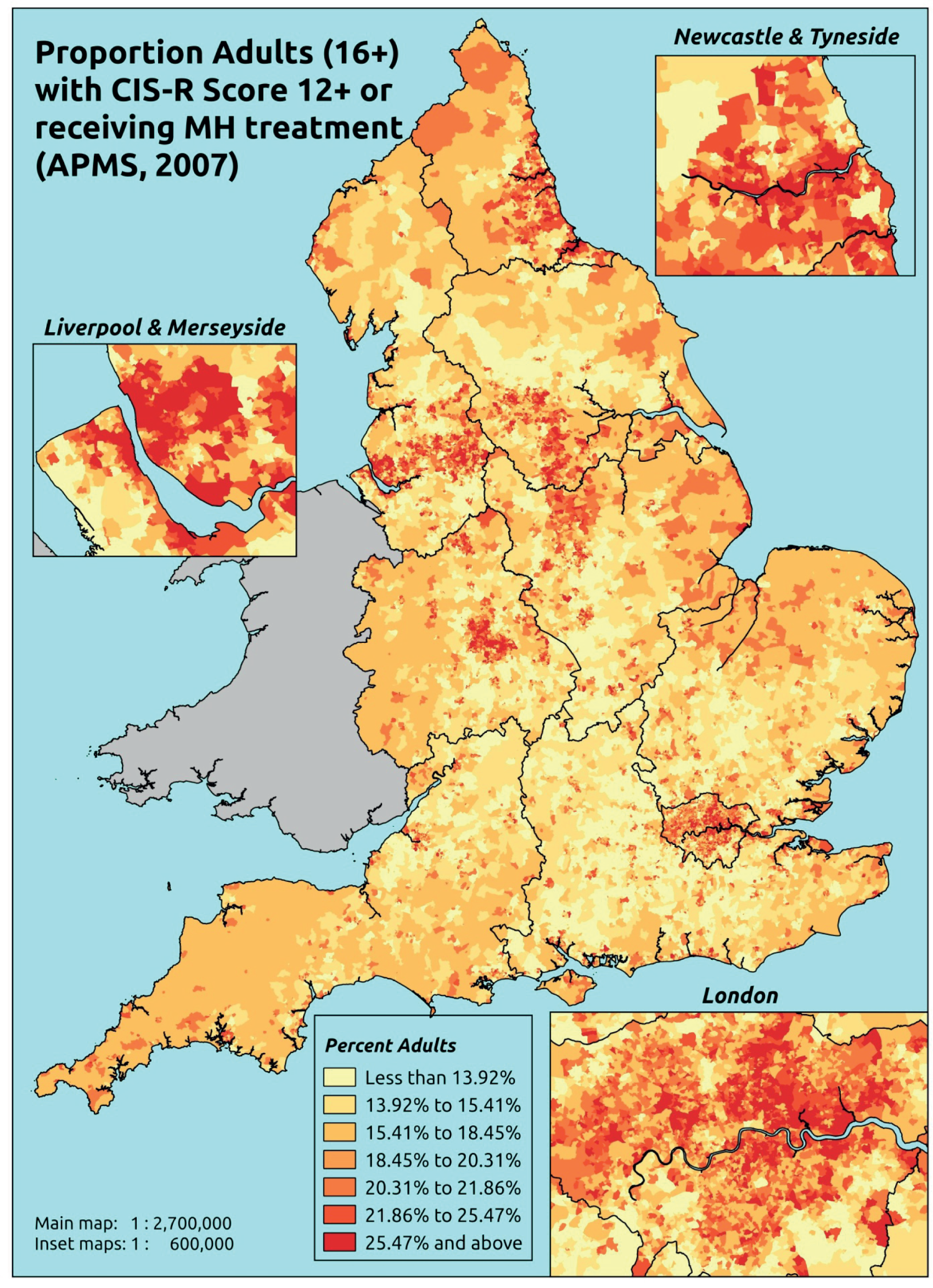
Response variable definition, provenance and prediction
This marker of mental health needs is derived from the CIS-R and questions about whether the respondent is currently receiving medication, counselling or therapy for a mental health problem. Here we estimate the proportion of people in each age–sex cohort, and overall for adults aged ≥ 16 years, with a CIS-R score of ≥ 12 (which is indicative of the presence of a common mental disorder) or who are currently receiving treatment for a mental health problem. This aims to capture individuals who would fall below the CIS-R ≥ 12 threshold because they are receiving treatment, and necessarily assumes that those who receive treatment do indeed need treatment. This marker of need is vulnerable to any sociodemographic or geographic variations in access to, or uptake of, care.
The APMS data set (n = 7403) comprises adults aged ≥ 16 years (living in England) and only surveyed one person per household, thus the analytical data set contains all respondents for whom data is available across all model response and predictor variables, namely CIS-R score, whether currently receiving treatment for a mental health problem, along with information on age band, sex, ethnicity, LLTI, tenure and IMD quintile of LSOA of residence (n = 7312).
| Age band (years) | Females | Age band (years) | Males | ||||
|---|---|---|---|---|---|---|---|
| Does not have condition | Has condition | % | Does not have condition | Has condition | % | ||
| 16–24 | 218 | 75 | 25.6 | 16–24 | 231 | 35 | 13.2 |
| 25–34 | 455 | 158 | 25.8 | 25–34 | 335 | 72 | 17.7 |
| 35–49 | 807 | 308 | 27.6 | 35–49 | 717 | 154 | 17.7 |
| 50–64 | 758 | 255 | 25.2 | 50–64 | 673 | 124 | 15.6 |
| 65–74 | 451 | 110 | 19.6 | 65–74 | 411 | 50 | 10.8 |
| 75–84 | 355 | 74 | 17.2 | 75–84 | 254 | 29 | 10.2 |
| ≥ 85 | 106 | 25 | 19.1 | ≥ 85 | 66 | 6 | 8.3 |
| Females | 3150 | 1005 | 24.2 | Males | 2687 | 470 | 14.9 |
| Total (males and females) | 5837 | 1475 | 20.2 | ||||
Model parameters are applied to microsimulated LSOA-level census data to produce estimates of the number (and proportion) of people expected to return a CIS-R score of ≥ 12 and/or be receiving treatment for a mental health problem in each age–sex cohort (and overall) in each of the 32,844 English LSOAs. As discussed in the report, bootstrapping is used to derive 95% CIs for the estimates. These LSOA-level prevalence rate estimates (and 95%CIs) are aggregated into a number of higher geographies, namely MSOAs, LAs, CCGs and regions (GORs). Proportionate attribution is used to restructure the prevalence rate estimates to align with 2001 MSOAs, as well as GP practice populations as defined by the 2011 NHS ADS.
Table 116 summarises how expected prevalence rates vary by age, sex and local deprivation (as measured by the 2010 IMD). There are 6569 LSOAs (with 9,226,227 adults) classified as being in the least deprived quintile; 6568 LSOAs (9,525,344 adults) in the second least deprived quintile; 6568 LSOAs (9,658,444 adults) in the third least deprived quintile; 6568 LSOAs (9,650,576 adults) in the fourth least deprived quintile; and 6568 LSOAs (9,535,167 adults) in the most deprived quintile. Note that, as a general rule, variations in prevalence rates reflect variations in the socioeconomic composition of populations in the different types of LSOA rather than variations in deprivation per se.
| Cohort | Least deprived quintile LSOAs | Second least deprived quintile LSOAs | Third least deprived quintile LSOAs | Fourth least deprived quintile LSOAs | Most deprived quintile LSOAs | All England |
|---|---|---|---|---|---|---|
| Female 16–24 | 18.4 (14.7 to 22.3) | 18.3 (14.8 to 22.2) | 24.8 (20.4 to 29.0) | 19.5 (16.1 to 24.0) | 25.9 (22.7 to 31.9) | 21.8 (18.5 to 26.0) |
| Female 25–34 | 20.4 (17.6 to 24.0) | 20.4 (18.0 to 23.4) | 27.4 (24.4 to 31.5) | 22.4 (19.7 to 26.4) | 29.6 (27.6 to 34.5) | 24.6 (23.0 to 28.0) |
| Female 35–49 | 21.0 (18.1 to 23.3) | 22.1 (19.5 to 24.1) | 29.9 (26.3 to 32.0) | 27.1 (23.7 to 29.8) | 35.1 (32.8 to 38.7) | 27.0 (24.8 to 28.6) |
| Female 50–64 | 17.4 (15.5 to 20.9) | 20.7 (18.8 to 23.9) | 27.5 (25.1 to 31.3) | 28.6 (26.1 to 32.8) | 35.7 (34.1 to 40.9) | 25.5 (23.9 to 28.4) |
| Female 65–74 | 12.3 (9.9 to 14.6) | 16.6 (13.6 to 19.0) | 21.6 (18.2 to 24.1) | 24.6 (20.7 to 27.9) | 27.9 (24.4 to 32.4) | 20.0 (17.5 to 22.2) |
| Female ≥ 75 | 11.4 (8.7 to 13.7) | 16.7 (12.6 to 19.4) | 20.3 (15.9 to 22.9) | 23.7 (18.7 to 26.8) | 24.2 (19.9 to 28.7) | 18.9 (15.5 to 21.0) |
| Females | 17.3 (14.7 to 20.2) | 19.7 (16.9 to 22.4) | 26.0 (22.7 to 29.2) | 24.8 (21.5 to 28.4) | 30.9 (28.3 to 35.6) | 23.8 (21.5 to 26.4) |
| Male 16–24 | 10.6 (7.9 to 12.8) | 10.9 (8.3 to 13.0) | 15.2 (11.8 to 17.9) | 12.5 (10.0 to 15.2) | 17.5 (14.7 to 21.3) | 13.6 (11.1 to 15.8) |
| Male 25–34 | 11.8 (9.4 to 13.8) | 12.2 (10.0 to 13.7) | 16.9 (14.0 to 19.4) | 14.1 (11.9 to 16.6) | 20.0 (18.2 to 23.6) | 15.5 (13.8 to 17.6) |
| Male 35–49 | 11.8 (9.3 to 13.5) | 13.0 (10.6 to 14.1) | 18.4 (15.0 to 19.8) | 17.6 (14.4 to 19.1) | 24.2 (21.6 to 27.0) | 17.1 (14.7 to 18.3) |
| Male 50–64 | 9.7 (8.2 to 11.5) | 12.1 (10.3 to 13.8) | 16.9 (14.9 to 19.1) | 18.7 (16.2 to 21.3) | 24.2 (22.1 to 28.1) | 15.9 (14.4 to 17.8) |
| Male 65–74 | 6.7 (5.2 to 7.9) | 9.6 (7.4 to 10.8) | 12.8 (10.0 to 14.6) | 15.5 (12.0 to 17.4) | 18.4 (14.8 to 21.0) | 12.1 (10.0 to 13.2) |
| Male ≥ 75 | 6.0 (4.3 to 7.3) | 9.3 (6.8 to 10.7) | 11.7 (8.6 to 13.4) | 14.3 (10.4 to 16.4) | 15.5 (11.9 to 18.3) | 10.9 (8.5 to 12.0) |
| Males | 9.8 (7.8 to 11.5) | 11.6 (9.3 to 13.0) | 16.0 (13.2 to 18.0) | 15.9 (13.0 to 18.1) | 21.1 (18.6 to 24.4) | 14.9 (12.9 to 16.5) |
| All | 13.7 (12.2 to 15.3) | 15.7 (14.0 to 16.9) | 21.2 (19.2 to 22.6) | 20.5 (18.3 to 22.3) | 26.1 (24.9 to 28.9) | 19.5 (18.5 to 20.4) |
| Factor (reference group) | Model coefficients | 95% CI | ||
|---|---|---|---|---|
| Estimate | SE | 2.5% CI | 97.5% | |
| (Intercept) | –1.68348 | 0.15765 | –1.99248 | –1.37448 |
| Age (16–24 years) | ||||
| 25–34 years | 0.12353 | 0.14025 | –0.15136 | 0.39841 |
| 35–49 years | 0.10458 | 0.13078 | –0.15174 | 0.36091 |
| 50–64 years | –0.29020 | 0.13680 | –0.55833 | –0.02206 |
| 65–74 years | –0.94469 | 0.15458 | –1.24767 | –0.64171 |
| 75–84 years | –1.31081 | 0.16946 | –1.64296 | –0.97867 |
| ≥ 85 years | –1.46498 | 0.24024 | –1.93585 | –0.99411 |
| Sex (females) | ||||
| Males | –0.69854 | 0.08529 | –0.86571 | –0.53138 |
| Ethnicity (white) | ||||
| Mixed | 0.06194 | 0.38014 | –0.68313 | 0.80701 |
| Black | –0.54233 | 0.25014 | –1.03261 | –0.05205 |
| Asian | –0.31027 | 0.25911 | –0.81814 | 0.19759 |
| Other | 0.51270 | 0.42471 | –0.31973 | 1.34514 |
| LLTI (no LTTI) | ||||
| LLTI | 1.10383 | 0.16984 | 0.77094 | 1.43672 |
| Tenure (owner–occupier) | ||||
| Social rent | 0.53020 | 0.09879 | 0.33657 | 0.72384 |
| Private rent or other tenure | 0.33443 | 0.12796 | 0.08363 | 0.58524 |
| LSOA deprivation quintile (least deprived quintile) | ||||
| Second LSOA deprivation quintile | –0.11887 | 0.13896 | –0.39123 | 0.15350 |
| Third LSOA deprivation quintile | 0.29091 | 0.13552 | 0.02530 | 0.55652 |
| Fourth LSOA deprivation quintile | –0.17998 | 0.14733 | –0.46875 | 0.10879 |
| Fifth LSOA deprivation quintile ( = most deprived) | 0.22540 | 0.14040 | –0.04977 | 0.50058 |
| Interaction effects | ||||
| LLTI and second LSOA deprivation quintile | 0.59927 | 0.22155 | 0.16502 | 1.03351 |
| LLTI and third LSOA deprivation quintile | 0.36408 | 0.21572 | –0.05873 | 0.78690 |
| LLTI and fourth LSOA deprivation quintile | 0.99885 | 0.22267 | 0.56242 | 1.43529 |
| LLTI and fifth LSOA deprivation quintile | 0.46431 | 0.21205 | 0.04868 | 0.87993 |
| Male and social rent | 0.38207 | 0.15588 | 0.07654 | 0.68761 |
| Male and private rent or other tenure | –0.11796 | 0.20796 | –0.52555 | 0.28964 |
| Mixed and LLTI | 0.29383 | 0.75672 | –1.18933 | 1.77699 |
| Black and LLTI | 1.20991 | 0.39160 | 0.44237 | 1.97745 |
| Asian and LLTI | 0.09235 | 0.40263 | –0.69681 | 0.88150 |
| Other and LLTI | –0.32211 | 0.77549 | –1.84207 | 1.19784 |
FIGURE 94.
Parameter plots: CIS-R score of ≥ 12 or any mental health treatment.

FIGURE 95.
Clinical Interview Schedule – Revised score of ≥ 12 or any mental health treatment: individual estimates and their 95% CIs. (a) MSOAs; (b) LAs; (c) CCGs; and (d) regions (GORs). MH, mental health.
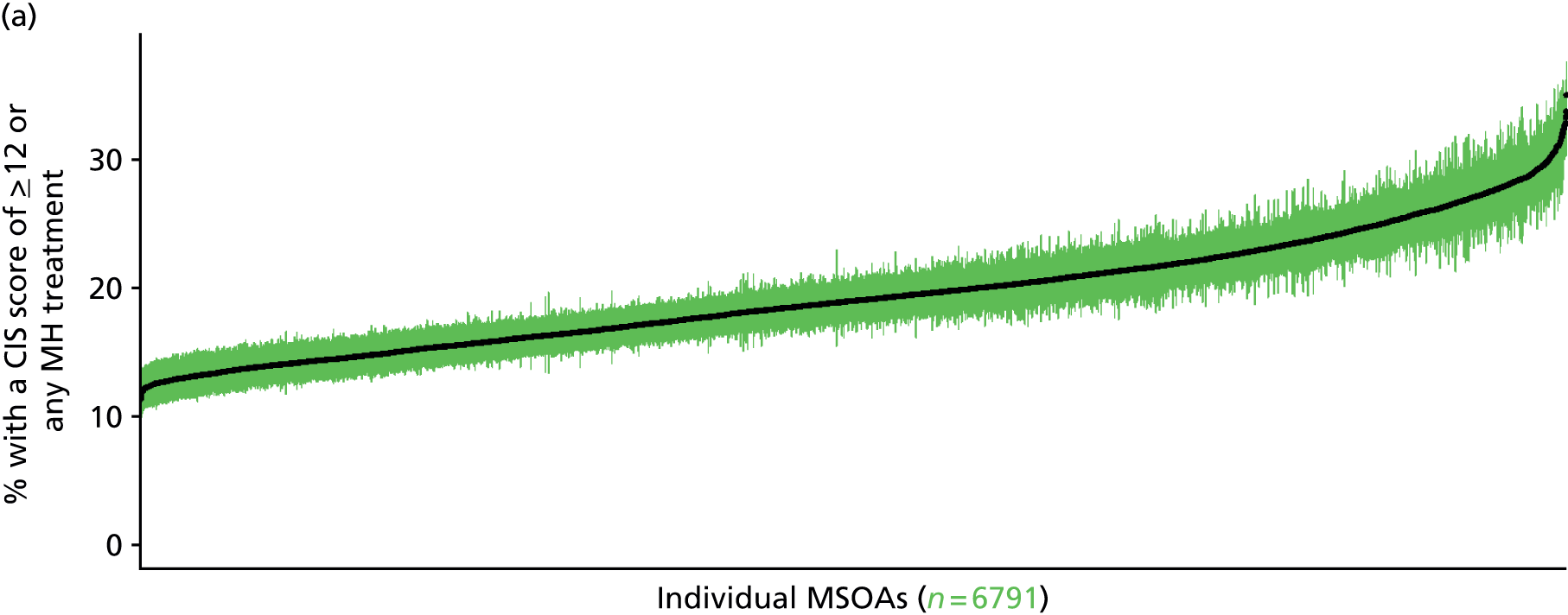
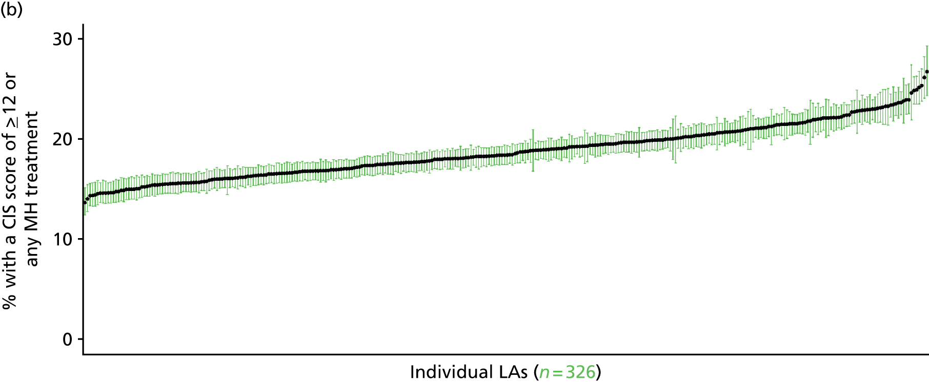
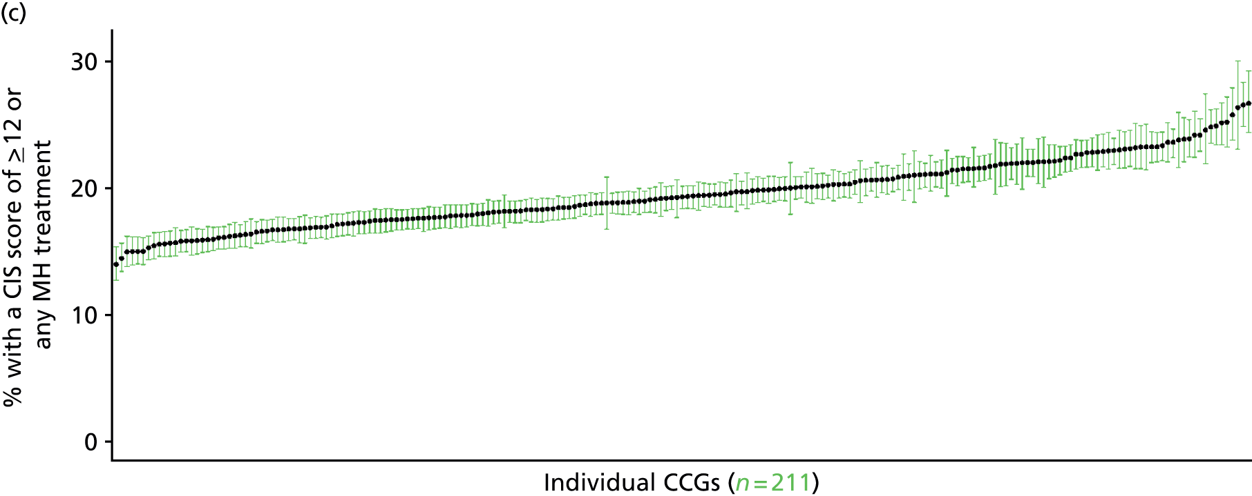
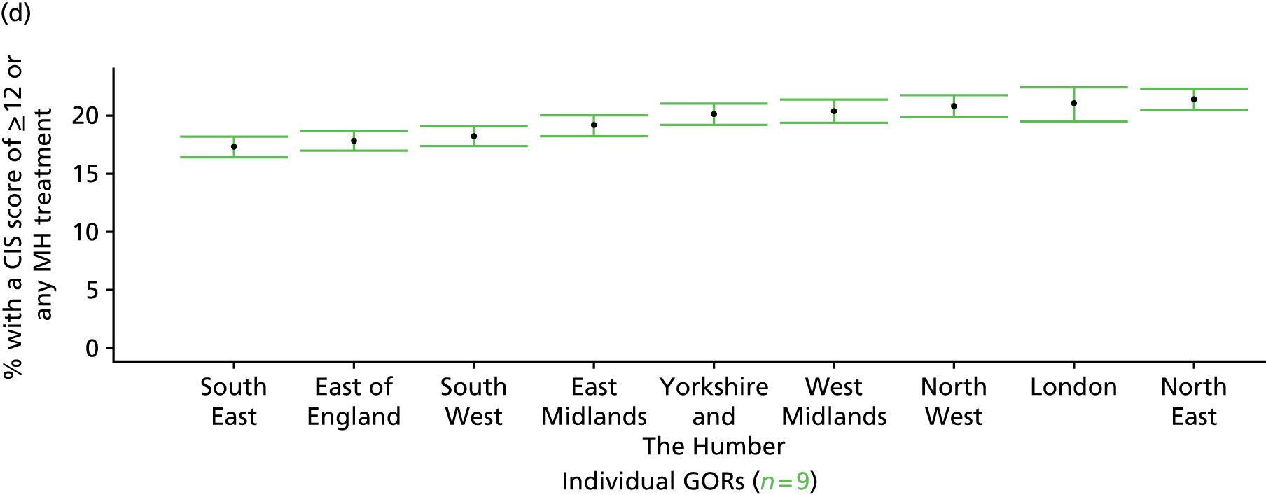
Clinical Interview Schedule – Revised score of ≥ 18 or any mental health treatment (Adult Psychiatry Morbidity Survey, 2007)
FIGURE 96.
Clinical Interview Schedule – Revised score of ≥ 18 or any mental health treatment: LSOA-level map. Contains Ordnance Survey data © Crown copyright and database right 2012.
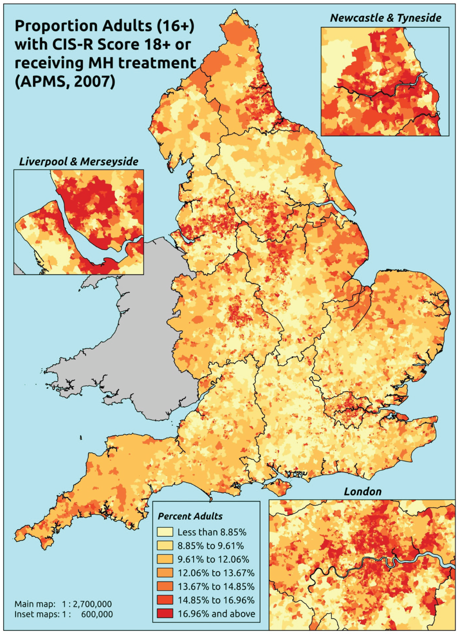
Response variable definition, provenance and prediction
This marker of mental health needs is derived from the CIS-R and questions about whether the respondent is currently receiving medication, counselling or therapy for a mental health problem. Here we estimate the proportion of people in each age–sex cohort, and overall for adults aged ≥ 16 years, with a CIS-R score of ≥ 18 (which is indicative of the presence of a common mental disorder which requires treatment) or who are currently receiving treatment for a mental health problem. This aims to capture individuals who would fall below the CIS-R ≥ 18 threshold because they are receiving treatment, and necessarily assumes that those who receive treatment do indeed need treatment. This marker of need is vulnerable to any sociodemographic or geographic variations in access to, or uptake of, care.
The APMS data set (n = 7403) comprises adults aged ≥ 16 years (living in England) and surveyed only one person per household, thus the analytical data set contains all respondents for whom data are available across all model response and predictor variables, namely CIS-R score and whether or not currently receiving treatment for a mental health problem, along with information on age band, sex, ethnicity, LLTI, tenure and IMD quintile of LSOA of residence (n = 7310).
| Age band (years) | Females | Age band (years) | Males | ||||
|---|---|---|---|---|---|---|---|
| Does not have condition | Has condition | % | Does not have condition | Has condition | % | ||
| 16–24 | 242 | 51 | 17.4 | 16–24 | 246 | 20 | 7.5 |
| 25–34 | 514 | 99 | 16.2 | 25–34 | 360 | 47 | 11.5 |
| 35–49 | 891 | 224 | 20.1 | 35–49 | 767 | 104 | 11.9 |
| 50–64 | 824 | 188 | 18.6 | 50–64 | 714 | 83 | 10.4 |
| 65–74 | 487 | 74 | 13.2 | 65–74 | 430 | 30 | 6.5 |
| 75–84 | 381 | 48 | 11.2 | 75–84 | 263 | 20 | 7.1 |
| ≥ 85 | 111 | 20 | 15.3 | ≥ 85 | 68 | 4 | 5.6 |
| Females | 3450 | 704 | 16.9 | Males | 2848 | 308 | 9.8 |
| Total (males and females) | 6298 | 1012 | 13.8 | ||||
Model parameters are applied to microsimulated LSOA-level census data to produce estimates of the number (and proportion) of people expected to return a CIS-R score of ≥ 18 and/or be receiving treatment for a mental health problem in each age–sex cohort (and overall) in each of the 32,844 English LSOAs. As discussed in the report, bootstrapping is used to derive 95% CIs for the estimates. These LSOA-level prevalence rate estimates (and 95% CIs) are aggregated into a number of higher geographies, namely MSOAs, LAs, CCGs and regions (GORs). Proportionate attribution is used to restructure the prevalence rate estimates to align with 2001 MSOAs, as well as GP practice populations as defined by the 2011 NHS ADS.
Table 119 summarises how expected prevalence rates vary by age, sex and local deprivation (as measured by the 2010 IMD). There are 6569 LSOAs (with 9,226,227 adults) classified as being in the least deprived quintile; 6568 LSOAs (9,525,344 adults) in the second least deprived quintile; 6568 LSOAs (9,658,444 adults) in the third least deprived quintile; 6568 LSOAs (9,650,576 adults) in the fourth least deprived quintile; and 6568 LSOAs (9,535,167 adults) in the most deprived quintile. Note that, as a general rule, variations in prevalence rates reflect variations in the socioeconomic composition of populations in the different types of LSOA rather than variations in deprivation per se.
| Cohort | Least deprived quintile LSOAs | Second least deprived quintile LSOAs | Third least deprived quintile LSOAs | Fourth least deprived quintile LSOAs | Most deprived quintile LSOAs | All England |
|---|---|---|---|---|---|---|
| Female 16–24 | 11.5 (8.3 to 14.5) | 10.7 (8.1 to 13.4) | 15.5 (11.6 to 19.1) | 13.0 (10.0 to 16.2) | 17.0 (13.7 to 21.0) | 13.9 (11.0 to 16.6) |
| Female 25–34 | 12.9 (10.5 to 15.1) | 11.7 (9.2 to 14.3) | 17.1 (14.1 to 20.4) | 14.7 (12.4 to 17.6) | 19.4 (16.4 to 22.9) | 15.6 (13.8 to 17.7) |
| Female 35–49 | 14.0 (11.6 to 16.3) | 14.2 (11.9 to 16.3) | 20.7 (18.1 to 23.1) | 20.3 (17.5 to 23.2) | 26.3 (23.5 to 29.6) | 19.1 (17.3 to 20.7) |
| Female 50–64 | 12.2 (10.3 to 14.5) | 13.7 (11.6 to 15.8) | 20.0 (17.3 to 22.6) | 21.2 (18.4 to 24.1) | 26.6 (23.3 to 29.9) | 18.3 (16.6 to 20.3) |
| Female 65–74 | 8.3 (6.4 to 10.2) | 10.0 (8.0 to 12.2) | 14.5 (11.7 to 17.9) | 15.7 (12.8 to 19.7) | 18.1 (15.1 to 22.1) | 12.9 (10.9 to 15.2) |
| Female ≥ 75 | 7.6 (5.9 to 10.2) | 10.4 (8.0 to 13.6) | 14.5 (11.4 to 18.2) | 16.0 (12.7 to 20.3) | 16.7 (13.9 to 20.7) | 12.8 (10.8 to 15.3) |
| Females | 11.5 (9.3 to 13.9) | 12.3 (10.0 to 14.7) | 17.8 (14.9 to 20.8) | 17.5 (14.7 to 20.7) | 21.8 (18.7 to 25.3) | 16.2 (14.2 to 18.3) |
| Male 16–24 | 6.1 (4.2 to 7.8) | 5.8 (4.3 to 7.5) | 8.8 (6.5 to 11.4) | 7.8 (5.8 to 10.0) | 10.7 (8.2 to 13.5) | 8.1 (6.2 to 9.9) |
| Male 25–34 | 6.7 (5.1 to 8.1) | 6.3 (4.9 to 7.6) | 9.5 (7.4 to 11.7) | 8.3 (6.6 to 10.1) | 11.6 (9.5 to 13.8) | 8.9 (7.5 to 10.2) |
| Male 35–49 | 7.3 (5.5 to 8.7) | 7.6 (6.3 to 9.0) | 11.8 (9.9 to 13.6) | 12.1 (10.4 to 13.9) | 16.9 (14.7 to 19.1) | 11.2 (9.8 to 12.5) |
| Male 50–64 | 6.3 (4.9 to 7.7) | 7.3 (6.0 to 8.5) | 11.3 (9.4 to 13.3) | 12.6 (10.3 to 14.6) | 16.6 (13.9 to 19.2) | 10.6 (9.2 to 12.0) |
| Male 65–74 | 4.2 (3.0 to 5.3) | 5.3 (4.1 to 6.5) | 8.0 (6.2 to 10.0) | 8.9 (7.0 to 11.3) | 10.9 (8.6 to 13.4) | 7.2 (5.7 to 8.6) |
| Male ≥ 75 | 3.8 (2.7 to 5.2) | 5.3 (4.1 to 7.3) | 7.7 (5.8 to 9.7) | 8.8 (6.7 to 11.7) | 9.7 (7.6 to 12.6) | 6.8 (5.5 to 8.3) |
| Males | 6.0 (4.5 to 7.4) | 6.6 (5.3 to 8.0) | 10.1 (8.1 to 12.1) | 10.3 (8.3 to 12.3) | 13.7 (11.3 to 16.1) | 9.4 (7.9 to 10.8) |
| All | 8.9 (7.4 to 10.1) | 9.5 (8.4 to 10.8) | 14.1 (12.3 to 15.6) | 14.0 (12.2 to 15.6) | 17.9 (16.0 to 19.7) | 12.9 (12.2 to 13.6) |
| Factor (reference group) | Model coefficients | 95% CI | ||
|---|---|---|---|---|
| Estimate | SE | 2.5% CI | 97.5% | |
| (Intercept) | –2.31263 | 0.20850 | –2.72129 | –1.90398 |
| Age (16–24 years) | ||||
| 25–34 years | 0.19518 | 0.19615 | –0.18927 | 0.57963 |
| 35–49 years | 0.14380 | 0.18540 | –0.21958 | 0.50719 |
| 50–64 years | –0.10894 | 0.20156 | –0.50399 | 0.28611 |
| 65–74 years | –0.51284 | 0.25723 | –1.01701 | –0.00867 |
| 75–84 years | –1.41425 | 0.44525 | –2.28693 | –0.54156 |
| ≥ 85 years | –0.12348 | 0.55127 | –1.20396 | 0.95700 |
| Sex (females) | ||||
| Males | –0.73218 | 0.10316 | –0.93437 | –0.52999 |
| Ethnicity (white) | ||||
| Mixed | 0.10262 | 0.38631 | –0.65454 | 0.85979 |
| Black | –0.39185 | 0.22539 | –0.83362 | 0.04992 |
| Asian | –0.21892 | 0.22371 | –0.65739 | 0.21954 |
| Other | –0.41120 | 0.50627 | –1.40349 | 0.58109 |
| LLTI (no LTTI) | ||||
| LLTI | 1.47531 | 0.37731 | 0.73578 | 2.21484 |
| Tenure (owner–occupier) | ||||
| Social rent | 0.56185 | 0.10960 | 0.34704 | 0.77666 |
| Private rent or other tenure | 0.37678 | 0.14652 | 0.08960 | 0.66397 |
| LSOA deprivation quintile (least deprived quintile) | ||||
| Second LSOA deprivation quintile | –0.25193 | 0.17587 | –0.59664 | 0.09278 |
| Third LSOA deprivation quintile | 0.20440 | 0.16740 | –0.12371 | 0.53251 |
| Fourth LSOA deprivation quintile | –0.16427 | 0.18041 | –0.51788 | 0.18934 |
| Fifth LSOA deprivation quintile ( = most deprived) | 0.19090 | 0.17055 | –0.14339 | 0.52518 |
| Interaction effects | ||||
| LLTI and second LSOA deprivation quintile | 0.61900 | 0.26352 | 0.10250 | 1.13549 |
| LLTI and third LSOA deprivation quintile | 0.48951 | 0.25077 | –0.00199 | 0.98102 |
| LLTI and fourth LSOA deprivation quintile | 0.92920 | 0.25832 | 0.42290 | 1.43551 |
| LLTI and fifth LSOA deprivation quintile | 0.50110 | 0.24419 | 0.02248 | 0.97971 |
| Male and social rent | 0.37532 | 0.17608 | 0.03019 | 0.72044 |
| Male and private rent or other tenure | –0.21954 | 0.25150 | –0.71248 | 0.27341 |
| 25–34 years and LLTI | –0.48083 | 0.38120 | –1.22797 | 0.26632 |
| 35–49 years and LLTI | –0.02367 | 0.34952 | –0.70874 | 0.66139 |
| 50–64 years and LLTI | –0.32654 | 0.35459 | –1.02154 | 0.36846 |
| 65–74 years and LLTI | –0.77812 | 0.39941 | –1.56096 | 0.00472 |
| 75–84 years and LLTI | –0.08373 | 0.54302 | –1.14805 | 0.98058 |
| ≥ 85 years and LLTI | –1.51723 | 0.66443 | –2.81952 | –0.21494 |
FIGURE 97.
Parameter plots: CIS-R score of ≥ 18 or any mental health treatment.

FIGURE 98.
Clinical Interview Schedule – Revised score of ≥ 18 or any mental health treatment: individual estimates and their 95% CIs. (a) MSOAs; (b) LAs; (c) CCGs; and (d) regions (GORs).


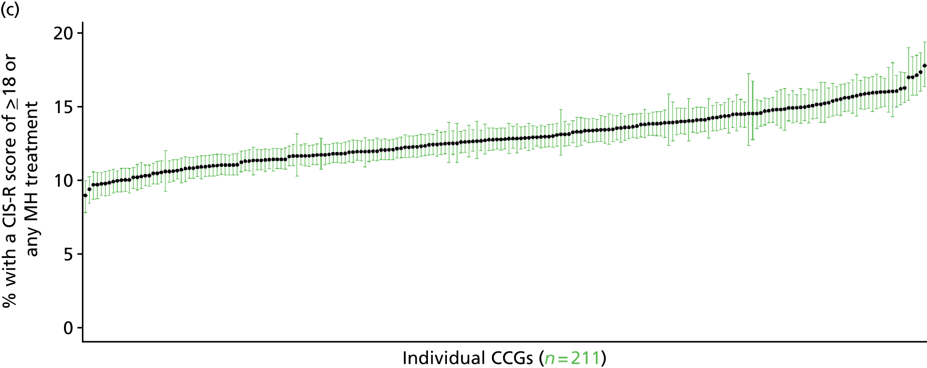
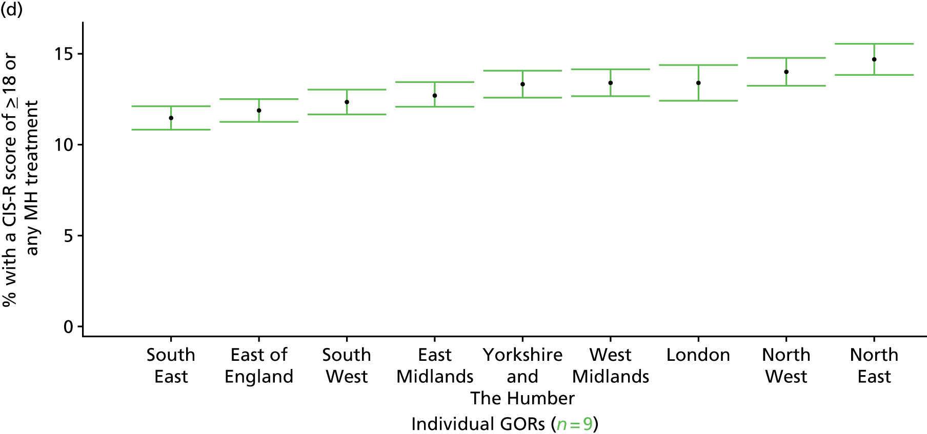
Generalised anxiety disorder symptoms in past week (Adult Psychiatry Morbidity Survey, 2007)
FIGURE 99.
Generalised anxiety disorder symptoms: LSOA-level map. Contains Ordnance Survey data © Crown copyright and database right 2012.
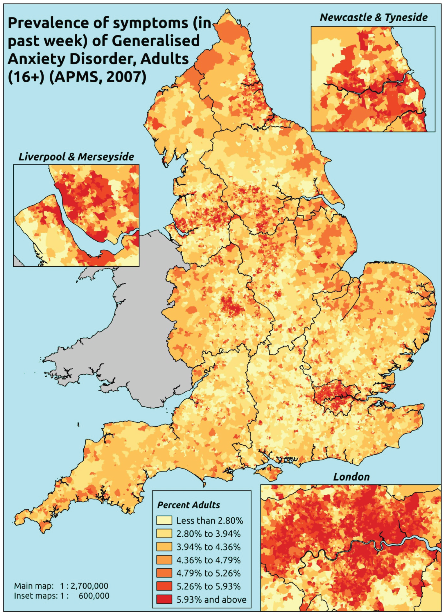
Response variable definition, provenance and prediction
On the basis of responses to the CIS-R, the APMS reports whether or not respondents had shown symptoms of generalised anxiety disorder [International Classification of Diseases, Tenth Edition (ICD-10): F41.1488] during the previous week. This is not entirely independent of sociodemographic or geographic variations in access to, or uptake of, care, as individuals may be free of symptoms because they are currently being treated for a generalised anxiety disorder. We cannot produce an alternative measure capturing underlying levels of generalised anxiety disorder because information of treatment (medication or otherwise) is not specific to this condition.
The APMS data set (n = 7403) comprises adults aged ≥ 16 years (living in England) and surveyed only one person per household; thus, the analytical data set contains all respondents for whom data are available across all model response and predictor variables, namely CIS-R question responses, age band, sex, ethnicity, LLTI, tenure and IMD quintile of LSOA of residence (n = 7326).
| Age band (years) | Females | Age band (years) | Males | ||||
|---|---|---|---|---|---|---|---|
| Does not have condition | Has condition | % | Does not have condition | Has condition | % | ||
| 16–24 | 274 | 19 | 6.5 | 16–24 | 261 | 5 | 1.9 |
| 25–34 | 586 | 28 | 4.6 | 25–34 | 386 | 21 | 5.2 |
| 35–49 | 1036 | 80 | 7.2 | 35–49 | 827 | 44 | 5.1 |
| 50–64 | 947 | 66 | 6.5 | 50–64 | 763 | 34 | 4.3 |
| 65–74 | 538 | 24 | 4.3 | 65–74 | 448 | 13 | 2.8 |
| 75–84 | 422 | 13 | 3.0 | 75–84 | 281 | 5 | 1.7 |
| ≥ 85 | 130 | 3 | 2.3 | ≥ 85 | 71 | 1 | 1.4 |
| Females | 3933 | 233 | 5.6 | Males | 3037 | 123 | 3.9 |
| Total (males and females) | 6970 | 356 | 4.9 | ||||
Model parameters are applied to microsimulated LSOA-level census data to produce estimates of the number (and proportion) of people expected to have shown symptoms of generalised anxiety disorder (ICD-10: F41.1488) during the previous week in each age–sex cohort (and overall) in each of the 32,844 English LSOAs. As discussed in the report, bootstrapping is used to derive 95% CIs for the estimates. These LSOA-level prevalence rate estimates (and 95% CIs) are aggregated into a number of higher geographies; namely MSOAs, LAs, CCGs and regions (GORs). Proportionate attribution is used to restructure the prevalence rate estimates to align with 2001 MSOAs, as well as GP practice populations as defined by the 2011 NHS ADS.
Table 123 summarises how expected prevalence rates vary by age, sex and local deprivation (as measured by the 2010 IMD). There are 6569 LSOAs (with 9,226,227 adults) classified as being in the least deprived quintile; 6568 LSOAs (9,525,344 adults) in the second least deprived quintile; 6568 LSOAs (9,658,444 adults) in the third least deprived quintile; 6568 LSOAs (9,650,576 adults) in the fourth least deprived quintile; and 6568 LSOAs (9,535,167 adults) in the most deprived quintile. Note that, as a general rule, variations in prevalence rates reflect variations in the socioeconomic composition of populations in the different types of LSOA rather than variations in deprivation per se.
| Cohort | Least deprived quintile LSOAs | Second least deprived quintile LSOAs | Third least deprived quintile LSOAs | Fourth least deprived quintile LSOAs | Most deprived quintile LSOAs | All England |
|---|---|---|---|---|---|---|
| Female 16–24 | 3.0 (1.7 to 4.3) | 4.3 (2.7 to 6.0) | 5.3 (3.4 to 7.3) | 4.5 (2.6 to 6.3) | 5.4 (3.3 to 7.2) | 4.6 (2.9 to 6.0) |
| Female 25–34 | 3.2 (2.0 to 4.4) | 4.5 (3.3 to 6.3) | 5.6 (4.0 to 7.5) | 4.9 (3.3 to 6.4) | 6.0 (4.5 to 8.0) | 5.0 (3.8 to 6.3) |
| Female 35–49 | 4.2 (2.9 to 5.6) | 6.2 (4.7 to 8.0) | 7.9 (6.3 to 9.8) | 7.3 (5.7 to 9.1) | 9.4 (7.4 to 11.4) | 7.0 (6.0 to 8.1) |
| Female 50–64 | 3.8 (2.7 to 5.0) | 5.7 (4.5 to 7.4) | 7.3 (5.9 to 9.5) | 6.8 (5.1 to 8.9) | 9.0 (7.1 to 11.2) | 6.4 (5.4 to 7.7) |
| Female 65–74 | 2.6 (1.6 to 3.6) | 3.9 (2.5 to 5.2) | 5.0 (3.2 to 6.9) | 4.5 (2.9 to 6.3) | 5.8 (3.8 to 7.9) | 4.3 (2.9 to 5.6) |
| Female ≥ 75 | 1.8 (1.0 to 2.6) | 2.6 (1.4 to 3.8) | 3.3 (1.8 to 4.5) | 2.7 (1.5 to 3.9) | 3.3 (1.9 to 4.7) | 2.7 (1.6 to 3.8) |
| Females | 3.3 (2.2 to 4.5) | 4.9 (3.5 to 6.5) | 6.2 (4.5 to 8.0) | 5.5 (3.9 to 7.3) | 7.0 (5.2 to 9.0) | 5.4 (4.2 to 6.6) |
| Male 16–24 | 1.9 (1.0 to 2.8) | 2.7 (1.6 to 3.7) | 3.4 (2.0 to 4.7) | 2.9 (1.7 to 4.1) | 3.6 (2.1 to 5.0) | 3.0 (1.8 to 4.1) |
| Male 25–34 | 1.9 (1.1 to 2.7) | 2.9 (1.8 to 3.9) | 3.6 (2.4 to 4.9) | 3.1 (2.1 to 4.1) | 4.1 (2.8 to 5.3) | 3.2 (2.1 to 4.2) |
| Male 35–49 | 2.6 (1.6 to 3.5) | 4.0 (2.7 to 5.2) | 5.2 (3.9 to 6.7) | 4.9 (3.7 to 6.2) | 6.8 (5.2 to 8.5) | 4.7 (3.7 to 5.7) |
| Male 50–64 | 2.5 (1.7 to 3.3) | 4.0 (3.0 to 5.2) | 5.2 (4.0 to 7.0) | 5.1 (3.8 to 6.6) | 6.9 (5.0 to 8.8) | 4.6 (3.7 to 5.8) |
| Male 65–74 | 1.9 (1.2 to 2.7) | 3.0 (1.9 to 4.2) | 3.9 (2.5 to 5.3) | 3.6 (2.2 to 5.0) | 4.7 (3.0 to 6.4) | 3.3 (2.2 to 4.4) |
| Male ≥ 75 | 1.5 (0.8 to 2.1) | 2.2 (1.1 to 3.2) | 2.7 (1.5 to 3.7) | 2.3 (1.2 to 3.2) | 2.8 (1.6 to 4.1) | 2.2 (1.3 to 3.0) |
| Males | 2.2 (1.4 to 3.0) | 3.4 (2.2 to 4.5) | 4.3 (3.0 to 5.7) | 4.0 (2.8 to 5.2) | 5.3 (3.7 to 6.8) | 3.8 (2.8 to 4.9) |
| All | 2.8 (2.0 to 3.5) | 4.1 (3.2 to 5.1) | 5.3 (4.3 to 6.3) | 4.8 (3.7 to 5.7) | 6.2 (5.1 to 7.3) | 4.6 (4.2 to 5.0) |
| Factor (reference group) | Model coefficients | 95% CI | ||
|---|---|---|---|---|
| Estimate | SE | 2.5% CI | 97.5% | |
| (Intercept) | –3.89407 | 0.28512 | –4.4529 | –3.33523 |
| Age (16–24 years) | ||||
| 25–34 years | 0.02509 | 0.26284 | –0.49007 | 0.54025 |
| 35–49 years | 0.26883 | 0.23955 | –0.20069 | 0.73835 |
| 50–64 years | –0.05993 | 0.24951 | –0.54898 | 0.42911 |
| 65–74 years | –0.74005 | 0.28506 | –1.29876 | –0.18134 |
| 75–84 years | –1.35781 | 0.33418 | –2.01280 | –0.70282 |
| ≥ 85 years | –1.80545 | 0.55852 | –2.90015 | –0.71074 |
| Sex (females) | ||||
| Males | –0.62822 | 0.19739 | –1.0151 | –0.24134 |
| Ethnicity (white) | ||||
| Mixed | 0.86821 | 0.45406 | –0.02174 | 1.75816 |
| Black | 0.45458 | 0.27028 | –0.07516 | 0.98432 |
| Asian | 0.41929 | 0.27905 | –0.12764 | 0.96622 |
| Other | 0.29891 | 0.62335 | –0.92285 | 1.52067 |
| LLTI (no LTTI) | ||||
| LLTI | 1.51032 | 0.14999 | 1.21634 | 1.80431 |
| Tenure (owner–occupier) | ||||
| Social rent | 0.69269 | 0.13728 | 0.42362 | 0.96177 |
| Private rent or other tenure | 0.31761 | 0.18595 | –0.04686 | 0.68208 |
| LSOA deprivation quintile (least deprived quintile) | ||||
| Second LSOA deprivation quintile | 0.33703 | 0.20710 | –0.06889 | 0.74295 |
| Third LSOA deprivation quintile | 0.48127 | 0.20280 | 0.08378 | 0.87875 |
| Fourth LSOA deprivation quintile | 0.19639 | 0.21119 | –0.21754 | 0.61033 |
| Fifth LSOA deprivation quintile ( = most deprived) | 0.24171 | 0.20830 | –0.16656 | 0.64997 |
| Interaction effects | ||||
| Male and LLTI | 0.46475 | 0.24650 | –0.01840 | 0.94789 |
FIGURE 100.
Parameter plots: generalised anxiety disorder symptoms.
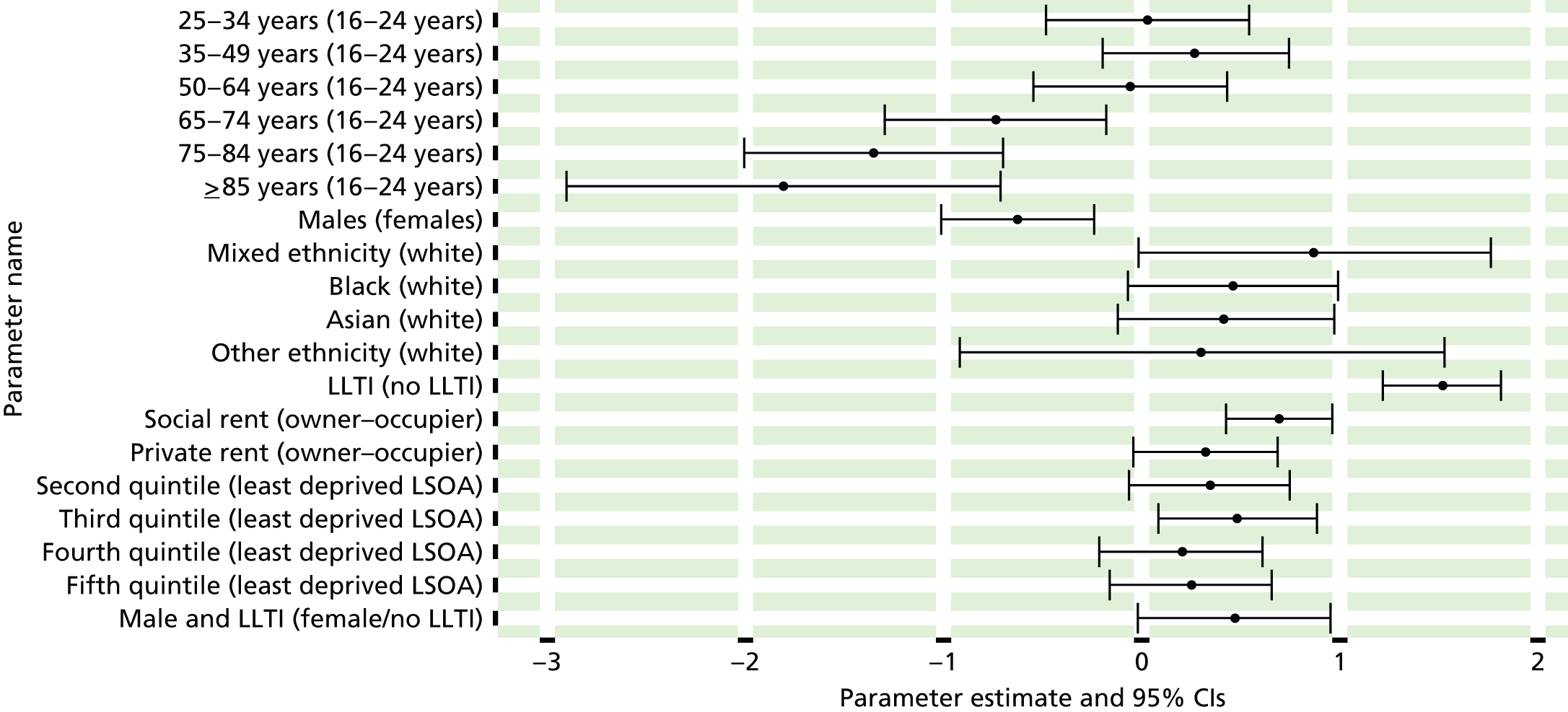
FIGURE 101.
Generalised anxiety disorder symptoms: individual estimates and their 95% CIs. (a) MSOAs; (b) LAs; (c) CCGs; and (d) regions (GORs). GAD, generalised anxiety disorder.
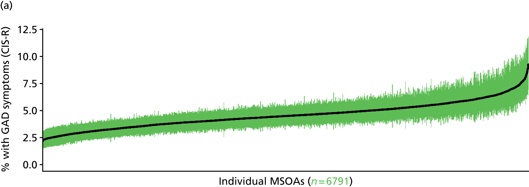
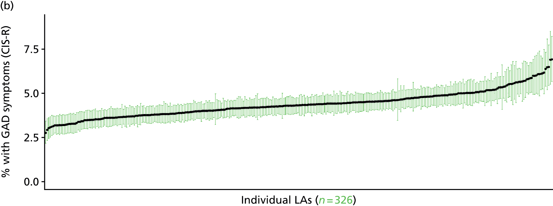
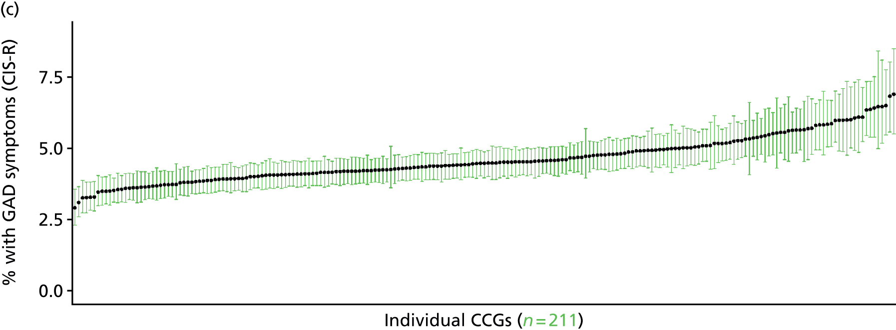

Mixed anxiety/depressive disorder symptoms in past week (Adult Psychiatry Morbidity Survey, 2007)
FIGURE 102.
Mixed anxiety/depressive disorder symptoms: LSOA-level map. Contains Ordnance Survey data © Crown copyright and database right 2012.

Response variable definition, provenance and prediction
On the basis of responses to the CIS-R, the APMS reports whether or not respondents had shown symptoms of mixed anxiety/depressive disorder (F41.2) during the previous week. This is not entirely independent of sociodemographic or geographic variations in access to, or uptake of, care, as individuals may be free of symptoms because they are currently being treated for a mixed anxiety/depressive disorder. We cannot produce an alternative measure capturing underlying levels of mixed anxiety/depressive disorder because information of treatment (medication or otherwise) is not specific to this condition.
The APMS data set (n = 7403) comprises adults aged ≥ 16 years (living in England) and surveyed only one person per household; thus, the analytical data set contains all respondents for whom data are available across all model response and predictor variables, namely CIS-R question responses, age band, sex, ethnicity, LLTI, tenure and IMD quintile of LSOA of residence (n = 7326).
| Age band (years) | Females | Age band (years) | Males | ||||
|---|---|---|---|---|---|---|---|
| Does not have condition | Has condition | % | Does not have condition | Has condition | % | ||
| 16–24 | 258 | 35 | 11.9 | 16–24 | 246 | 20 | 7.5 |
| 25–34 | 531 | 83 | 13.5 | 25–34 | 376 | 31 | 7.6 |
| 35–49 | 991 | 125 | 11.2 | 35–49 | 805 | 66 | 7.6 |
| 50–64 | 908 | 105 | 10.4 | 50–64 | 744 | 53 | 6.6 |
| 65–74 | 519 | 43 | 7.7 | 65–74 | 443 | 18 | 3.9 |
| 75–84 | 405 | 30 | 6.9 | 75–84 | 275 | 11 | 3.8 |
| ≥ 85 | 128 | 5 | 3.8 | ≥ 85 | 70 | 2 | 2.8 |
| Females | 3740 | 426 | 10.2 | Males | 2959 | 201 | 6.4 |
| Total (males and females) | 6699 | 627 | 8.6 | ||||
Model parameters are applied to microsimulated LSOA-level census data to produce estimates of the number (and proportion) of people expected to have shown symptoms of mixed anxiety/depressive disorder (F41.2) during the previous week in each age–sex cohort (and overall) in each of the 32,844 English LSOAs. As discussed in the report, bootstrapping is used to derive 95% CIs for the estimates. These LSOA-level prevalence rate estimates (and 95% CIs) are aggregated into a number of higher geographies; namely MSOAs, LAs, CCGs and regions (GORs). Proportionate attribution is used to restructure the prevalence rate estimates to align with 2001 MSOAs, as well as GP practice populations as defined by the 2011 NHS ADS.
Table 125 summarises how expected prevalence rates vary by age, sex and local deprivation (as measured by the 2010 IMD). There are 6569 LSOAs (with 9,226,227 adults) classified as being in the least deprived quintile; 6568 LSOAs (9,525,344 adults) in the second least deprived quintile; 6568 LSOAs (9,658,444 adults) in the third least deprived quintile; 6568 LSOAs (9,650,576 adults) in the fourth least deprived quintile; and 6568 LSOAs (9,535,167 adults) in the most deprived quintile. Note that, as a general rule, variations in prevalence rates reflect variations in the socioeconomic composition of populations in the different types of LSOA rather than variations in deprivation per se.
| Cohort | Least deprived quintile LSOAs | Second least deprived quintile LSOAs | Third least deprived quintile LSOAs | Fourth least deprived quintile LSOAs | Most deprived quintile LSOAs | All England |
|---|---|---|---|---|---|---|
| Female 16–24 | 8.6 (5.9 to 12.1) | 9.4 (6.9 to 12.4) | 12.9 (10.0 to 17.8) | 10.1 (7.8 to 13.9) | 13.3 (10.1 to 17.5) | 11.1 (8.8 to 14.5) |
| Female 25–34 | 10.6 (7.6 to 12.8) | 11.0 (8.0 to 13.1) | 15.5 (11.8 to 19.1) | 11.9 (8.8 to 14.5) | 15.6 (12.2 to 18.4) | 13.2 (10.7 to 15.3) |
| Female 35–49 | 8.1 (6.0 to 10.2) | 9.5 (7.2 to 11.2) | 12.6 (10.6 to 15.7) | 10.8 (9.1 to 13.0) | 15.1 (12.9 to 17.7) | 11.2 (9.8 to 13.0) |
| Female 50–64 | 6.6 (5.2 to 8.4) | 9.0 (7.2 to 10.7) | 10.8 (8.7 to 13.5) | 10.5 (8.6 to 12.7) | 15.2 (12.5 to 18.0) | 10.2 (8.8 to 11.7) |
| Female 65–74 | 3.8 (2.5 to 5.3) | 6.9 (5.2 to 8.8) | 7.0 (5.0 to 9.1) | 7.9 (5.6 to 10.6) | 11.8 (8.8 to 14.9) | 7.2 (5.5 to 9.0) |
| Female ≥ 75 | 3.5 (2.2 to 4.7) | 6.2 (4.4 to 8.1) | 5.8 (3.9 to 8.0) | 6.1 (4.0 to 7.9) | 8.3 (6.1 to 11.2) | 5.9 (4.2 to 7.4) |
| Females | 6.9 (5.0 to 8.8) | 8.7 (6.6 to 10.7) | 11.0 (8.7 to 14.1) | 10.0 (7.8 to 12.5) | 13.9 (11.1 to 16.9) | 10.1 (8.4 to 12.1) |
| Male 16–24 | 5.0 (3.4 to 7.7) | 5.6 (4.0 to 7.8) | 7.7 (5.8 to 11.2) | 6.1 (4.5 to 8.3) | 8.4 (6.3 to 11.0) | 6.7 (5.4 to 8.9) |
| Male 25–34 | 6.1 (4.0 to 7.9) | 6.5 (4.4 to 8.1) | 9.2 (6.6 to 12.2) | 7.1 (5.1 to 9.1) | 9.6 (7.0 to 12.1) | 7.9 (6.0 to 9.5) |
| Male 35–49 | 4.7 (3.3 to 6.1) | 5.7 (4.2 to 6.7) | 7.6 (6.0 to 9.7) | 6.8 (5.3 to 8.5) | 10.0 (8.2 to 11.8) | 7.0 (5.8 to 8.3) |
| Male 50–64 | 4.0 (3.0 to 5.1) | 5.8 (4.5 to 7.0) | 6.9 (5.4 to 8.7) | 7.1 (5.4 to 8.7) | 10.6 (8.4 to 12.9) | 6.7 (5.5 to 7.9) |
| Male 65–74 | 2.6 (1.7 to 3.5) | 4.9 (3.5 to 6.2) | 4.9 (3.3 to 6.3) | 5.7 (3.9 to 7.5) | 8.7 (6.1 to 11.0) | 5.2 (3.8 to 6.3) |
| Male ≥ 75 | 2.5 (1.6 to 3.4) | 4.4 (2.9 to 5.9) | 4.1 (2.6 to 5.5) | 4.4 (2.8 to 5.7) | 6.2 (4.0 to 8.4) | 4.2 (2.9 to 5.5) |
| Males | 4.2 (2.9 to 5.6) | 5.6 (4.1 to 6.9) | 7.0 (5.2 to 9.2) | 6.5 (4.8 to 8.3) | 9.4 (7.2 to 11.7) | 6.5 (5.2 to 8.0) |
| All | 5.6 (4.4 to 6.6) | 7.2 (6.0 to 8.2) | 9.1 (7.9 to 10.8) | 8.3 (6.9 to 9.5) | 11.7 (10.1 to 13.1) | 8.4 (7.8 to 9.0) |
| Factor (reference group) | Model coefficients | 95% CI | ||
|---|---|---|---|---|
| Estimate | SE | 2.5% CI | 97.5% | |
| (Intercept) | –2.46357 | 0.22673 | –2.90796 | –2.01918 |
| Age (16–24 years) | ||||
| 25–34 years | 0.30158 | 0.19982 | –0.09008 | 0.69323 |
| 35–49 years | –0.08291 | 0.19579 | –0.46665 | 0.30083 |
| 50–64 years | –0.40855 | 0.21729 | –0.83443 | 0.01733 |
| 65–74 years | –1.72903 | 0.39538 | –2.50396 | –0.95409 |
| 75–84 years | –0.92594 | 0.38064 | –1.67199 | –0.17989 |
| ≥ 85 years | –13.0749 | 200.8464 | –406.734 | 380.5841 |
| Sex (females) | ||||
| Males | –0.63127 | 0.12654 | –0.87928 | –0.38326 |
| Ethnicity (white) | ||||
| Mixed | –0.78236 | 0.60033 | –1.95901 | 0.39429 |
| Black | –0.08558 | 0.23361 | –0.54346 | 0.37231 |
| Asian | –0.21076 | 0.26135 | –0.72301 | 0.30150 |
| Other | 0.90961 | 0.39611 | 0.13323 | 1.68599 |
| LLTI (no LTTI) | ||||
| LLTI | 0.59406 | 0.44123 | –0.27076 | 1.45887 |
| Tenure (owner–occupier) | ||||
| Social rent | 0.39707 | 0.10975 | 0.18197 | 0.61218 |
| Private rent or other tenure | 0.14257 | 0.13949 | –0.13082 | 0.41597 |
| LSOA deprivation quintile (least deprived quintile) | ||||
| Second LSOA deprivation quintile | –0.03640 | 0.19520 | –0.41899 | 0.34618 |
| Third LSOA deprivation quintile | 0.40504 | 0.18717 | 0.03818 | 0.77189 |
| Fourth LSOA deprivation quintile | 0.02306 | 0.20057 | –0.37006 | 0.41618 |
| Fifth LSOA deprivation quintile ( = most deprived) | 0.29116 | 0.19336 | –0.08783 | 0.67015 |
| Interaction effects | ||||
| 25–34 years and LLTI | –0.87494 | 0.43544 | –1.72841 | –0.02147 |
| 35–49 years and LLTI | –0.10978 | 0.38917 | –0.87255 | 0.65299 |
| 50–64 years and LLTI | 0.03258 | 0.39591 | –0.74341 | 0.80856 |
| 65–74 years and LLTI | 0.98292 | 0.52478 | –0.04566 | 2.01149 |
| 75–84 years and LLTI | –0.34243 | 0.52579 | –1.37298 | 0.68812 |
| ≥ 85 years and LLTI | 11.29915 | 200.8471 | –382.361 | 404.9594 |
| Male and LLTI | 0.30969 | 0.18258 | –0.04816 | 0.66755 |
| LLTI and second LSOA deprivation quintile | 0.72095 | 0.31946 | 0.09481 | 1.34708 |
| LLTI and third LSOA deprivation quintile | 0.09488 | 0.31552 | –0.52354 | 0.71330 |
| LLTI and fourth LSOA deprivation quintile | 0.54179 | 0.32101 | –0.08740 | 1.17097 |
| LLTI and fifth LSOA deprivation quintile | 0.54286 | 0.30290 | –0.05082 | 1.13654 |
FIGURE 103.
Parameter plots: mixed anxiety/depressive disorder symptoms.
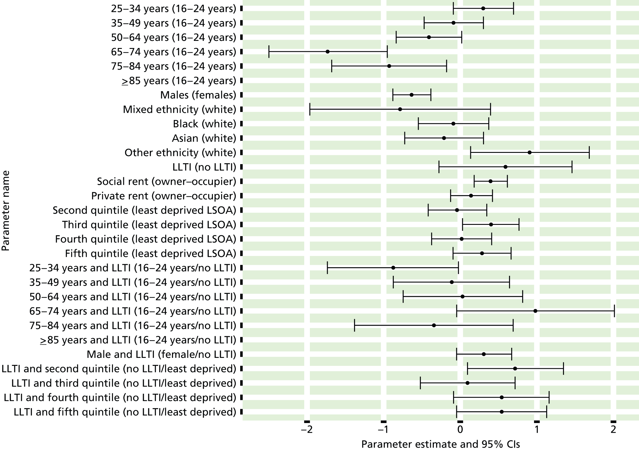
FIGURE 104.
Mixed anxiety/depressive disorder symptoms: individual estimates and their 95% CIs. (a) MSOAs; (b) LAs; (c) CCGs; and (d) regions (GORs). MADD, mixed anxiety/depressive disorder.

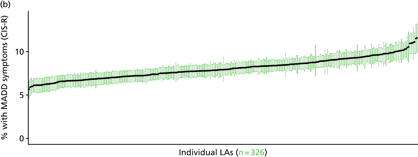
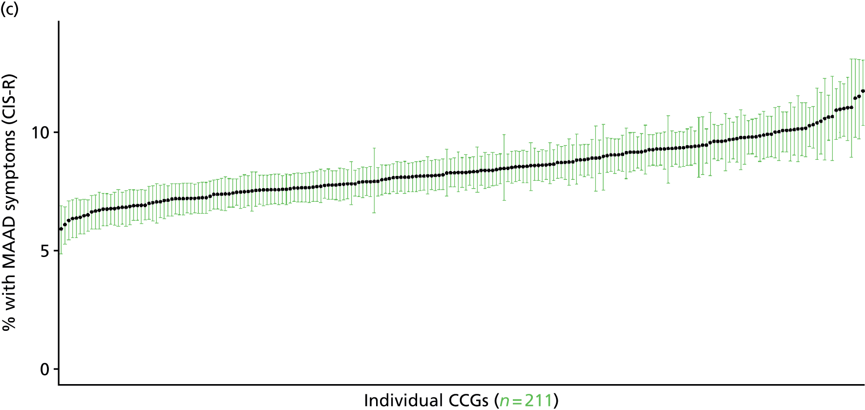
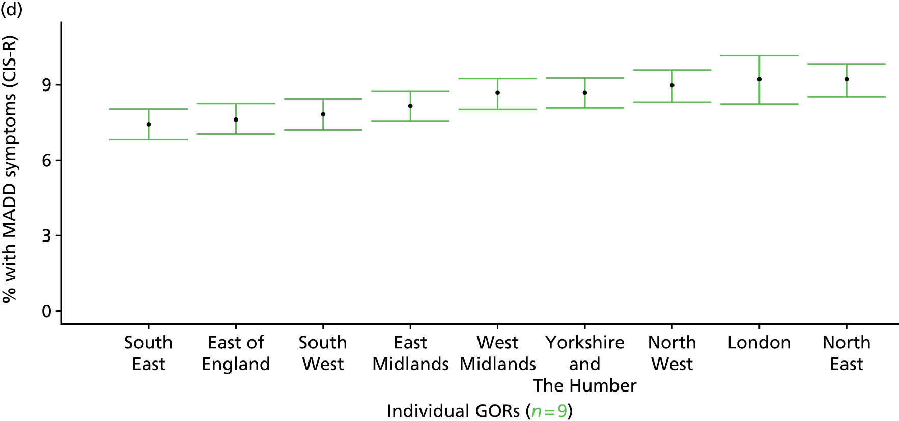
Depressive episode symptoms in past week (Adult Psychiatry Morbidity Survey, 2007)
FIGURE 105.
Depressive episode symptoms: LSOA-level map. Contains Ordnance Survey data © Crown copyright and database right 2012.

Response variable definition, provenance and prediction
On the basis of responses to the CIS-R, the APMS reports whether or not respondents had shown symptoms of a depressive episode (F32) during the previous week. This is not entirely independent of sociodemographic or geographic variations in access to, or uptake of, care, as individuals may be free of symptoms because they are currently being treated for depression. We cannot produce an alternative measure capturing underlying levels of depression because information of treatment (medication or otherwise) is not specific to this condition.
The APMS data set (n = 7403) comprises adults ≥ 16 years (living in England) and surveyed only one person per household; thus, the analytical data set contains all respondents for whom data are available across all model response and predictor variables, namely CIS-R question responses, age band, sex, ethnicity, LLTI, tenure and IMD quintile of LSOA of residence (n = 7326).
| Age band (years) | Females | Age band (years) | Males | ||||
|---|---|---|---|---|---|---|---|
| Does not have condition | Has condition | % | Does not have condition | Has condition | % | ||
| 16–24 | 281 | 12 | 4.1 | 16–24 | 260 | 6 | 2.3 |
| 25–34 | 594 | 20 | 3.3 | 25–34 | 393 | 14 | 3.4 |
| 35–49 | 1048 | 68 | 6.1 | 35–49 | 842 | 29 | 3.3 |
| 50–64 | 976 | 37 | 3.7 | 50–64 | 769 | 28 | 3.5 |
| 65–74 | 546 | 16 | 2.8 | 65–74 | 457 | 4 | 0.9 |
| 75–84 | 425 | 10 | 2.3 | 75–84 | 283 | 3 | 1.0 |
| ≥ 85 | 131 | 2 | 1.5 | ≥ 85 | 70 | 2 | 2.8 |
| Females | 4001 | 165 | 4.0 | Males | 3074 | 86 | 2.7 |
| Total (males and females) | 7075 | 251 | 3.4 | ||||
Model parameters are applied to microsimulated LSOA-level census data to produce estimates of the number (and proportion) of people expected to have shown symptoms of a depressive episode (F32) during the previous week in each age–sex cohort (and overall) in each of the 32,844 English LSOAs. As discussed in the report, bootstrapping is used to derive 95% CIs for the estimates. These LSOA-level prevalence rate estimates (and 95% CIs) are aggregated into a number of higher geographies; namely MSOAs, LAs, CCGs and regions (GORs). Proportionate attribution is used to restructure the prevalence rate estimates to align with 2001 MSOAs, as well as GP practice populations as defined by the 2011 NHS ADS.
Table 128 summarises how expected prevalence rates vary by age, sex and local deprivation (as measured by the 2010 IMD). There are 6569 LSOAs (with 9,226,227 adults) classified as being in the least deprived quintile; 6568 LSOAs (9,525,344 adults) in the second least deprived quintile; 6568 LSOAs (9,658,444 adults) in the third least deprived quintile; 6568 LSOAs (9,650,576 adults) in the fourth least deprived quintile; and 6568 LSOAs (9,535,167 adults) in the most deprived quintile. Note that, as a general rule, variations in prevalence rates reflect variations in the socioeconomic composition of populations in the different types of LSOA rather than variations in deprivation per se.
| Cohort | Least deprived quintile LSOAs | Second least deprived quintile LSOAs | Third least deprived quintile LSOAs | Fourth least deprived quintile LSOAs | Most deprived quintile LSOAs | All England |
|---|---|---|---|---|---|---|
| Female 16–24 | 2.8 (1.5 to 4.5) | 2.1 (1.1 to 3.3) | 2.6 (1.5 to 4.1) | 4.8 (2.8 to 7.3) | 4.7 (2.8 to 6.9) | 3.6 (2.2 to 5.2) |
| Female 25–34 | 2.5 (1.5 to 3.6) | 1.9 (1.1 to 2.7) | 2.3 (1.5 to 3.3) | 4.4 (3.0 to 5.9) | 4.6 (3.1 to 6.2) | 3.4 (2.3 to 4.3) |
| Female 35–49 | 3.7 (2.4 to 5.0) | 3.0 (1.8 to 4.1) | 3.9 (2.7 to 5.4) | 7.7 (5.8 to 9.7) | 8.6 (6.3 to 10.4) | 5.4 (4.2 to 6.3) |
| Female 50–64 | 2.8 (1.7 to 4.1) | 2.3 (1.5 to 3.2) | 3.1 (2.1 to 4.5) | 6.4 (4.8 to 8.3) | 7.2 (5.7 to 9.4) | 4.2 (3.4 to 5.3) |
| Female 65–74 | 1.7 (0.9 to 2.7) | 1.4 (0.8 to 2.2) | 1.8 (1.0 to 2.6) | 3.7 (2.0 to 5.4) | 3.9 (2.3 to 5.9) | 2.4 (1.4 to 3.4) |
| Female ≥ 75 | 1.9 (0.9 to 3.1) | 1.4 (0.7 to 2.3) | 1.7 (0.9 to 2.8) | 3.3 (1.8 to 5.6) | 3.3 (1.9 to 4.9) | 2.2 (1.4 to 3.5) |
| Females | 2.8 (1.6 to 4.0) | 2.2 (1.3 to 3.1) | 2.8 (1.8 to 4.0) | 5.5 (3.8 to 7.4) | 5.9 (4.2 to 7.8) | 3.8 (2.8 to 4.9) |
| Male 16–24 | 1.5 (0.7 to 2.4) | 1.1 (0.6 to 1.8) | 1.4 (0.7 to 2.4) | 2.8 (1.6 to 4.6) | 3.2 (1.8 to 4.8) | 2.1 (1.2 to 3.2) |
| Male 25–34 | 1.3 (0.7 to 2.0) | 1.0 (0.5 to 1.4) | 1.3 (0.8 to 1.9) | 2.5 (1.7 to 3.4) | 3.0 (2.0 to 4.2) | 2.0 (1.3 to 2.6) |
| Male 35–49 | 1.9 (1.2 to 2.8) | 1.6 (0.9 to 2.3) | 2.2 (1.4 to 3.1) | 4.7 (3.4 to 5.9) | 6.0 (4.3 to 7.6) | 3.3 (2.5 to 4.1) |
| Male 50–64 | 1.6 (1.0 to 2.5) | 1.4 (0.9 to 2.1) | 1.9 (1.2 to 2.9) | 4.3 (3.1 to 5.8) | 5.4 (4.0 to 7.1) | 2.8 (2.2 to 3.8) |
| Male 65–74 | 1.1 (0.6 to 1.7) | 0.9 (0.5 to 1.4) | 1.2 (0.7 to 1.8) | 2.7 (1.6 to 4.1) | 3.1 (1.9 to 4.6) | 1.7 (1.1 to 2.4) |
| Male ≥ 75 | 1.2 (0.6 to 2.0) | 0.9 (0.5 to 1.6) | 1.2 (0.6 to 2.0) | 2.5 (1.3 to 4.0) | 2.7 (1.6 to 4.2) | 1.6 (0.9 to 2.5) |
| Males | 1.5 (0.9 to 2.3) | 1.2 (0.7 to 1.9) | 1.7 (1.0 to 2.5) | 3.5 (2.4 to 4.9) | 4.3 (2.9 to 5.8) | 2.5 (1.7 to 3.3) |
| All | 2.2 (1.5 to 2.8) | 1.7 (1.2 to 2.2) | 2.2 (1.6 to 3.0) | 4.5 (3.6 to 5.5) | 5.1 (4.1 to 6.2) | 3.2 (2.8 to 3.6) |
| Factor (reference group) | Model coefficients | 95% CI | ||
|---|---|---|---|---|
| Estimate | SE | 2.5% CI | 97.5% | |
| (Intercept) | –3.98080 | 0.33425 | –4.63592 | –3.32567 |
| Age (16–24 years) | ||||
| 25–34 years | –0.15700 | 0.31105 | –0.76666 | 0.45265 |
| 35–49 years | 0.15994 | 0.27930 | –0.38750 | 0.70737 |
| 50–64 years | –0.45396 | 0.29431 | –1.03081 | 0.12290 |
| 65–74 years | –1.32688 | 0.35105 | –2.01494 | –0.63881 |
| 75–84 years | –1.66296 | 0.38976 | –2.42690 | –0.89903 |
| ≥ 85 years | –1.76210 | 0.57567 | –2.89041 | –0.63379 |
| Sex (females) | ||||
| Males | –0.93063 | 0.31252 | –1.54317 | –0.31810 |
| Ethnicity (white) | ||||
| Mixed | 1.15990 | 0.62362 | –0.06240 | 2.38219 |
| Black | –14.3174 | 442.1516 | –880.934 | 852.2997 |
| Asian | 0.34506 | 0.53114 | –0.69597 | 1.38610 |
| Other | 0.53783 | 1.03589 | –1.49251 | 2.56817 |
| LLTI (no LTTI) | ||||
| LLTI | 1.87951 | 0.19223 | 1.50273 | 2.25628 |
| Tenure (owner–occupier) | ||||
| Social rent | 0.50141 | 0.19307 | 0.12299 | 0.87982 |
| Private rent or other tenure | 0.24671 | 0.27844 | –0.29905 | 0.79246 |
| LSOA deprivation quintile (least deprived quintile) | ||||
| Second LSOA deprivation quintile | –0.34497 | 0.26678 | –0.86785 | 0.17791 |
| Third LSOA deprivation quintile | –0.18197 | 0.25312 | –0.67809 | 0.31415 |
| Fourth LSOA deprivation quintile | 0.41574 | 0.22935 | –0.03379 | 0.86528 |
| Fifth LSOA deprivation quintile ( = most deprived) | 0.27925 | 0.23336 | –0.17813 | 0.73663 |
| Interaction effects | ||||
| Male and social rent | 0.54560 | 0.30283 | –0.04795 | 1.13915 |
| Male and private rent | –0.69823 | 0.56199 | –1.79973 | 0.40326 |
| Mixed and LLTI | 0.74811 | 0.92559 | –1.06605 | 2.56226 |
| Black and LLTI | 14.84164 | 442.1518 | –851.776 | 881.4591 |
| Asian and LLTI | –0.86689 | 0.72015 | –2.27839 | 0.54460 |
| Other and LLTI | –16.9906 | 2008.587 | –3953.82 | 3919.84 |
| Male and LLTI | 0.58621 | 0.33840 | –0.07706 | 1.24947 |
FIGURE 106.
Parameter plots: depressive episode symptoms.
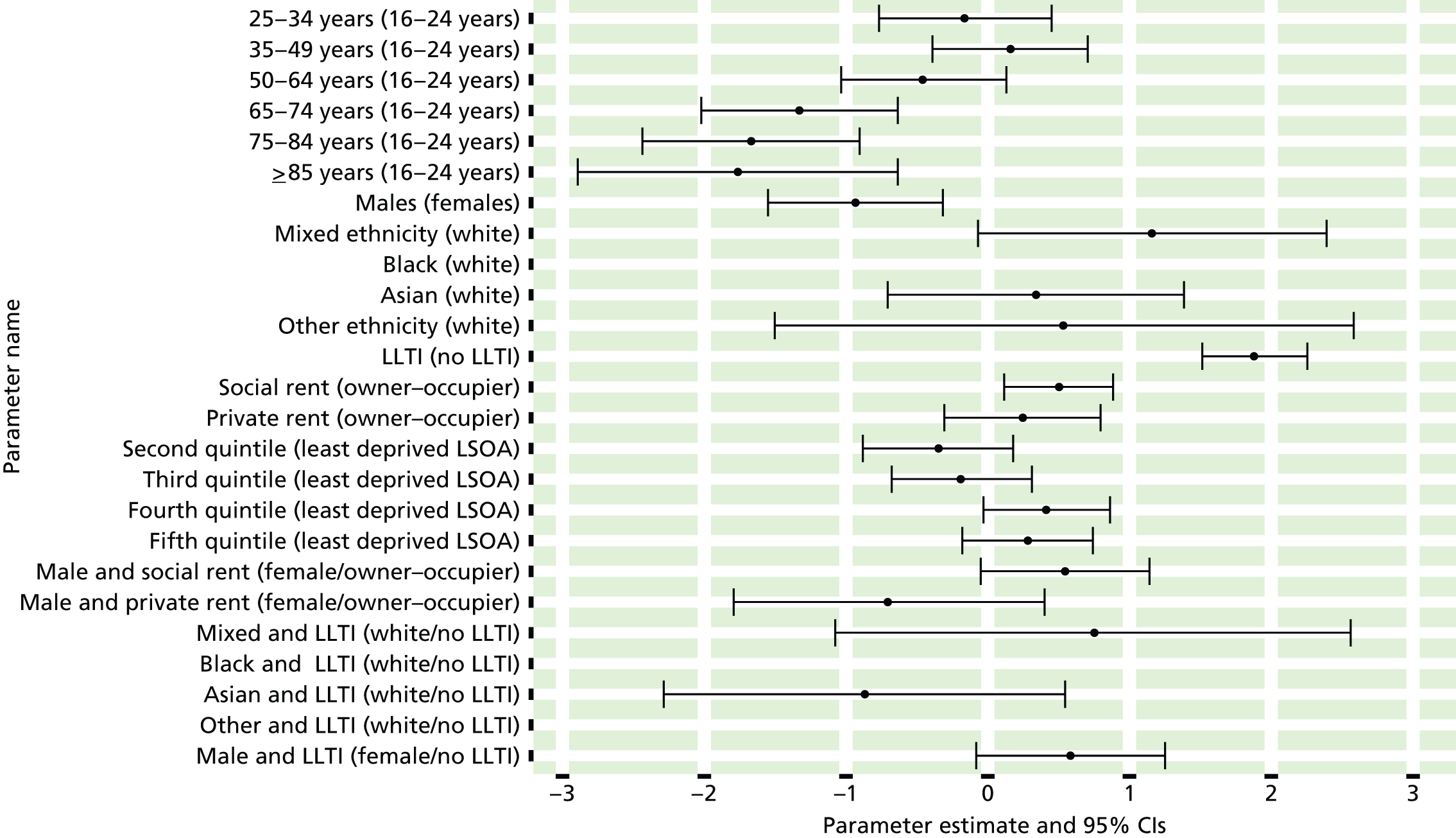
FIGURE 107.
Depressive episode symptoms: individual estimates and their 95% CIs. (a) MSOAs; (b) LAs; (c) CCGs; and (d) regions (GORs).
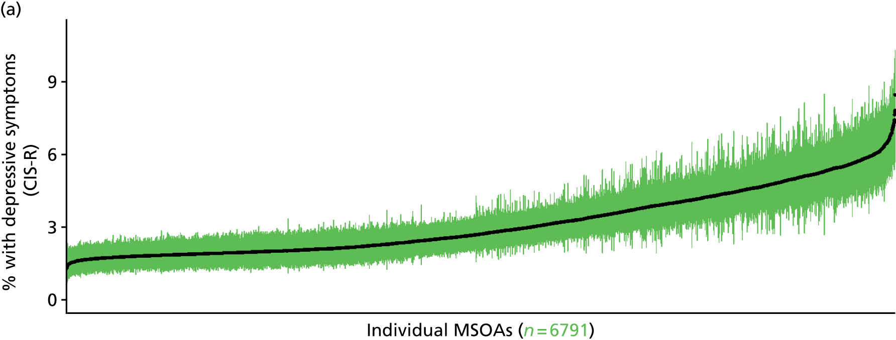
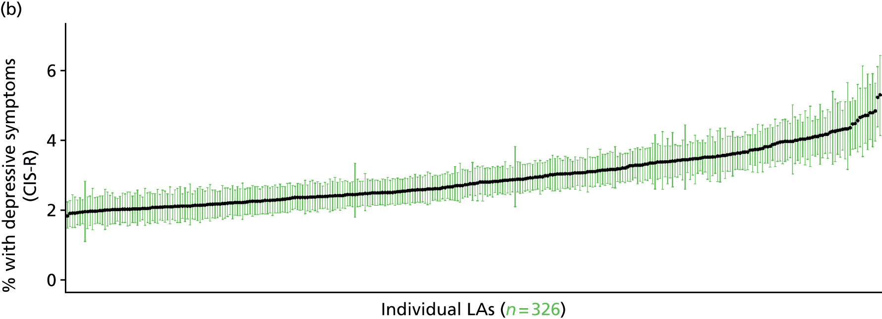
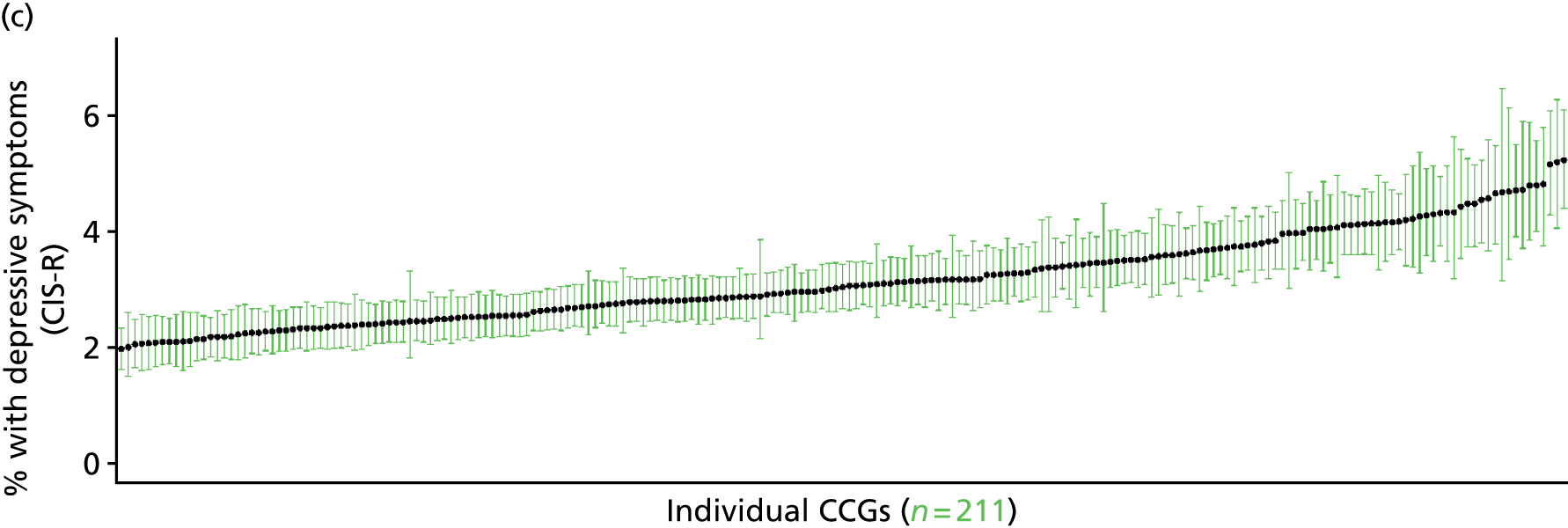
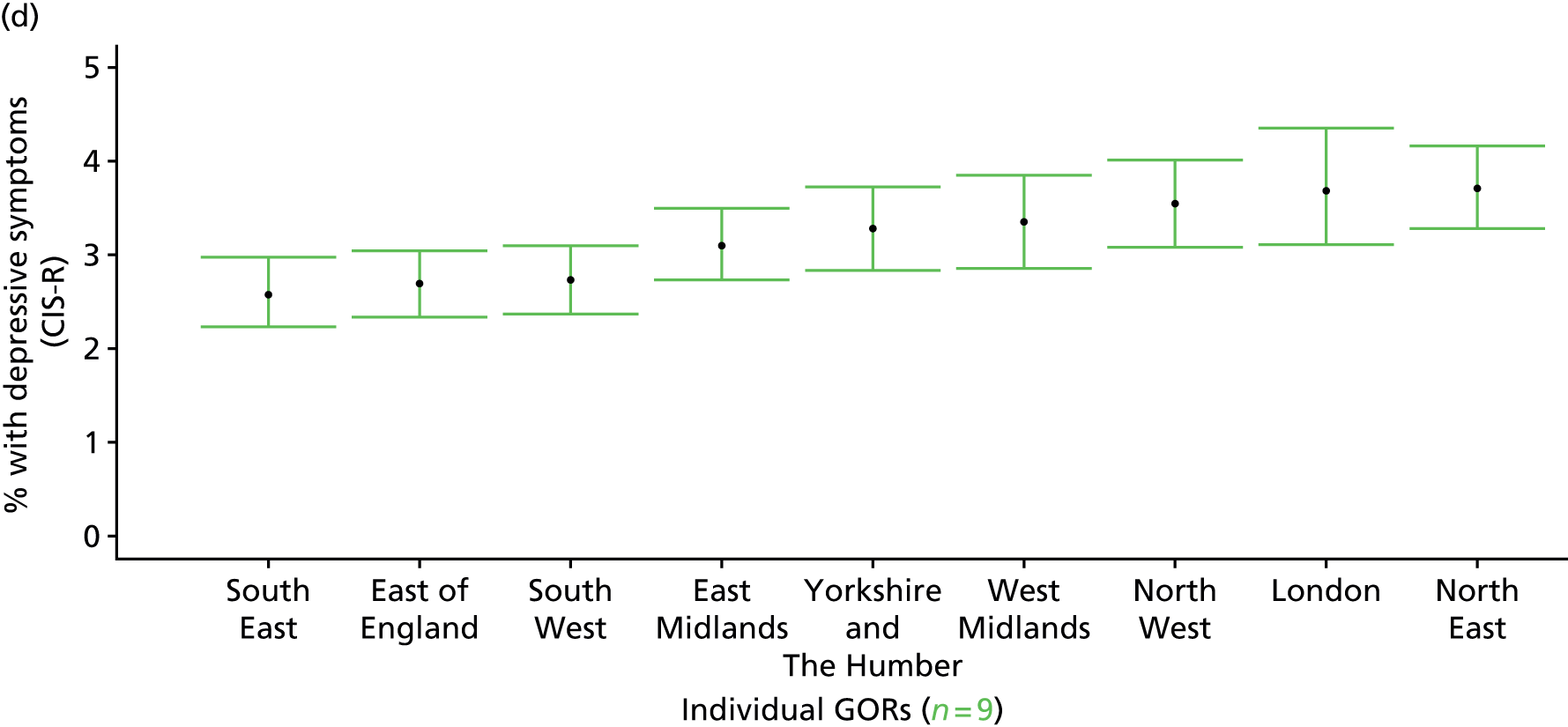
Symptoms of generalised anxiety disorder, mixed anxiety/depressive disorder or a depressive episode in past week (Adult Psychiatry Morbidity Survey, 2007)
FIGURE 108.
Symptoms of generalised anxiety disorder, mixed anxiety/depressive disorder or a depressive episode: LSOA-level map. Contains Ordnance Survey data © Crown copyright and database right 2012.
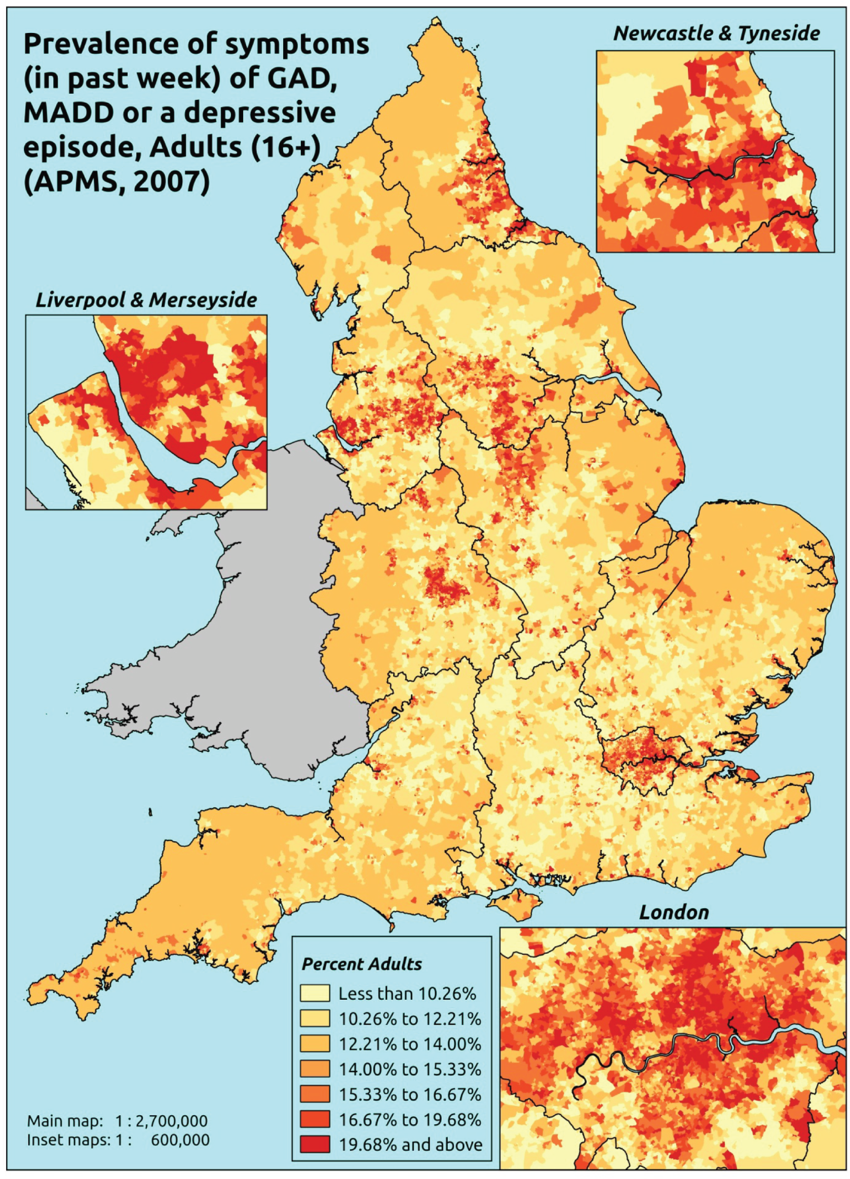
Response variable definition, provenance and prediction
On the basis of responses to the CIS-R, here we capture whether respondents to the APMS have shown symptoms of generalised anxiety disorder (ICD-10: F41.1488), mixed anxiety/depressive disorder (F41.2) or a depressive episode (F32) during the previous week. This is not entirely independent of sociodemographic or geographic variations in access to, or uptake of, care, as individuals may be free of symptoms because they are currently being treated for anxiety/depression. We cannot produce an alternative measure capturing underlying levels of anxiety/depression because information of treatment (medication or otherwise) is not specific to these conditions.
The APMS data set (n = 7403) comprises adults ≥ 16 years (living in England) and surveyed only one person per household; thus, the analytical data set contains all respondents for whom data are available across all model response and predictor variables, namely CIS-R question responses, age band, sex, ethnicity, LLTI, tenure and IMD quintile of LSOA of residence (n = 7326).
| Age band (years) | Females | Age band (years) | Males | ||||
|---|---|---|---|---|---|---|---|
| Does not have condition | Has condition | % | Does not have condition | Has condition | % | ||
| 16–24 | 231 | 62 | 21.2 | 16–24 | 236 | 30 | 11.3 |
| 25–34 | 488 | 126 | 20.5 | 25–34 | 349 | 58 | 14.3 |
| 35–49 | 875 | 241 | 21.6 | 35–49 | 742 | 129 | 14.8 |
| 50–64 | 823 | 190 | 18.8 | 50–64 | 695 | 102 | 12.8 |
| 65–74 | 484 | 78 | 13.9 | 65–74 | 427 | 34 | 7.4 |
| 75–84 | 386 | 49 | 11.3 | 75–84 | 268 | 18 | 6.3 |
| ≥ 85 | 123 | 10 | 7.5 | ≥ 85 | 68 | 4 | 5.6 |
| Females | 3410 | 756 | 18.1 | Males | 2785 | 375 | 11.9 |
| Total (males and females) | 6195 | 1131 | 15.4 | ||||
Model parameters are applied to microsimulated LSOA-level census data to produce estimates of the number (and proportion) of people expected to have shown symptoms of generalised anxiety disorder (ICD-10: F41.1488), mixed anxiety/depressive disorder (F41.2) or a depressive episode (F32) during the previous week in each age–sex cohort (and overall) in each of the 32,844 English LSOAs. As discussed in the report, bootstrapping is used to derive 95% CIs for the estimates. These LSOA-level prevalence rate estimates (and 95% CIs) are aggregated into a number of higher geographies; namely MSOAs, LAs, CCGs and regions (GORs). Proportionate attribution is used to restructure the prevalence rate estimates to align with 2001 MSOAs, as well as GP practice populations as defined by the 2011 NHS ADS.
Table 131 summarises how expected prevalence rates vary by age, sex and local deprivation (as measured by the 2010 IMD). There are 6569 LSOAs (with 9,226,227 adults) classified as being in the least deprived quintile; 6568 LSOAs (9,525,344 adults) in the second least deprived quintile; 6568 LSOAs (9,658,444 adults) in the third least deprived quintile; 6568 LSOAs (9,650,576 adults) in the fourth least deprived quintile; and 6568 LSOAs (9,535,167 adults) in the most deprived quintile. Note that, as a general rule, variations in prevalence rates reflect variations in the socioeconomic composition of populations in the different types of LSOA rather than variations in deprivation per se.
| Cohort | Least deprived quintile LSOAs | Second least deprived quintile LSOAs | Third least deprived quintile LSOAs | Fourth least deprived quintile LSOAs | Most deprived quintile LSOAs | All England |
|---|---|---|---|---|---|---|
| Female 16–24 | 14.8 (11.4 to 19.3) | 16.1 (12.7 to 20.2) | 20.5 (16.2 to 25.5) | 17.6 (14.2 to 21.8) | 21.7 (17.5 to 26.2) | 18.5 (15.2 to 22.2) |
| Female 25–34 | 15.7 (12.5 to 18.8) | 17.0 (13.8 to 20.5) | 21.5 (17.9 to 26.0) | 18.9 (16.2 to 22.1) | 23.7 (20.2 to 27.3) | 19.9 (17.6 to 22.6) |
| Female 35–49 | 15.9 (12.9 to 18.6) | 18.2 (15.4 to 20.8) | 22.9 (19.9 to 25.9) | 22.2 (19.4 to 25.0) | 28.3 (25.8 to 31.5) | 21.5 (19.6 to 23.6) |
| Female 50–64 | 12.5 (10.3 to 14.6) | 15.9 (14.0 to 18.4) | 19.5 (17.0 to 22.7) | 21.0 (18.6 to 24.0) | 27.5 (24.9 to 31.1) | 18.9 (17.1 to 21.0) |
| Female 65–74 | 8.1 (5.9 to 9.9) | 11.6 (9.2 to 13.7) | 13.4 (10.3 to 16.0) | 15.5 (12.2 to 17.9) | 20.0 (16.3 to 23.6) | 13.2 (10.9 to 15.3) |
| Female ≥ 75 | 6.1 (4.3 to 7.6) | 9.5 (7.0 to 12.1) | 10.1 (7.3 to 12.7) | 11.8 (8.4 to 14.7) | 14.4 (11.5 to 17.5) | 10.2 (7.9 to 12.0) |
| Females | 12.5 (9.9 to 15.0) | 15.2 (12.6 to 18.0) | 18.7 (15.6 to 22.2) | 18.8 (15.9 to 21.9) | 24.0 (20.8 to 27.6) | 17.9 (15.7 to 20.2) |
| Male 16–24 | 8.4 (5.9 to 10.6) | 9.3 (7.3 to 11.7) | 12.1 (9.4 to 15.1) | 11.1 (8.6 to 13.4) | 14.5 (12.0 to 17.5) | 11.4 (9.2 to 13.7) |
| Male 25–34 | 8.8 (6.4 to 10.3) | 9.9 (7.7 to 12.0) | 12.7 (10.2 to 15.1) | 11.8 (9.8 to 13.7) | 16.0 (13.4 to 18.4) | 12.4 (10.3 to 13.9) |
| Male 35–49 | 8.8 (6.7 to 10.7) | 10.7 (8.8 to 12.5) | 14.0 (11.7 to 16.1) | 14.5 (12.6 to 16.7) | 20.4 (18.0 to 23.1) | 13.7 (11.9 to 15.3) |
| Male 50–64 | 7.3 (5.8 to 8.6) | 10.1 (8.5 to 12.0) | 12.6 (10.6 to 15.1) | 14.7 (12.8 to 17.1) | 20.7 (18.5 to 23.8) | 12.7 (11.5 to 14.4) |
| Male 65–74 | 5.0 (3.5 to 6.3) | 7.8 (5.9 to 9.4) | 9.2 (6.6 to 11.3) | 11.3 (8.6 to 13.0) | 15.3 (12.1 to 18.4) | 9.3 (7.3 to 10.8) |
| Male ≥ 75 | 4.1 (2.8 to 5.1) | 6.6 (4.8 to 8.5) | 7.2 (5.1 to 9.0) | 8.8 (6.3 to 10.8) | 11.3 (8.6 to 14.2) | 7.3 (5.5 to 8.8) |
| Males | 7.4 (5.5 to 8.9) | 9.4 (7.6 to 11.4) | 12.0 (9.6 to 14.3) | 12.7 (10.6 to 14.8) | 17.5 (14.9 to 20.3) | 11.8 (10.1 to 13.5) |
| All | 10.0 (8.3 to 11.3) | 12.4 (10.8 to 13.9) | 15.5 (13.9 to 17.3) | 15.8 (14.4 to 17.4) | 20.8 (19.2 to 22.8) | 4.9 (14.0 to 15.7) |
| Factor (reference group) | Model coefficients | 95% CI | ||
|---|---|---|---|---|
| Estimate | SE | 2.5% CI | 97.5% | |
| (Intercept) | –1.94153 | 0.17425 | –2.28307 | –1.60000 |
| Age (16–24 years) | ||||
| 25–34 years | 0.04014 | 0.14955 | –0.25298 | 0.33326 |
| 35–49 years | 0.02324 | 0.13932 | –0.24982 | 0.29630 |
| 50–64 years | –0.39311 | 0.14652 | –0.68029 | –0.10592 |
| 65–74 years | –1.09920 | 0.16871 | –1.42988 | –0.76852 |
| 75–84 years | –1.54379 | 0.1891 | –1.91443 | –1.17316 |
| ≥ 85 years | –2.07120 | 0.31296 | –2.68459 | –1.45781 |
| Sex (females) | ||||
| Males | –0.76422 | 0.11815 | –0.99579 | –0.53264 |
| Ethnicity (white) | ||||
| Mixed | 0.35669 | 0.33243 | –0.29487 | 1.00826 |
| Black | 0.06141 | 0.18551 | –0.30218 | 0.42501 |
| Asian | –0.09125 | 0.20635 | –0.49569 | 0.31319 |
| Other | 0.77852 | 0.36457 | 0.06396 | 1.49309 |
| LLTI (no LTTI) | ||||
| LLTI | 1.02786 | 0.1962 | 0.64331 | 1.41242 |
| Tenure (owner–occupier) | ||||
| Social rent | 0.49385 | 0.10645 | 0.28520 | 0.70250 |
| Private rent or other tenure | 0.24494 | 0.13891 | –0.02732 | 0.51720 |
| LSOA deprivation quintile (least deprived quintile) | ||||
| Second LSOA deprivation quintile | –0.02011 | 0.15681 | –0.32745 | 0.28724 |
| Third LSOA deprivation quintile | 0.28607 | 0.15462 | –0.01697 | 0.58912 |
| Fourth LSOA deprivation quintile | –0.03346 | 0.16348 | –0.35389 | 0.28696 |
| Fifth LSOA deprivation quintile ( = most deprived) | 0.17192 | 0.15929 | –0.14028 | 0.48413 |
| Interaction effects | ||||
| Male and LLTI | 0.36556 | 0.14929 | 0.07294 | 0.65817 |
| LLTI and second LSOA deprivation quintile | 0.52515 | 0.24613 | 0.04274 | 1.00757 |
| LLTI and third LSOA deprivation quintile | 0.21691 | 0.24157 | –0.25657 | 0.69039 |
| LLTI and fourth LSOA deprivation quintile | 0.67404 | 0.24517 | 0.19352 | 1.15457 |
| LLTI and fifth LSOA deprivation quintile | 0.58203 | 0.23381 | 0.12376 | 1.04029 |
| Male and social rent | 0.33888 | 0.17000 | 0.00568 | 0.67208 |
| Male and private rent or other tenure | –0.06480 | 0.22831 | –0.51229 | 0.38269 |
FIGURE 109.
Parameter plots: symptoms of generalised anxiety disorder, mixed anxiety/depressive disorder or a depressive episode.
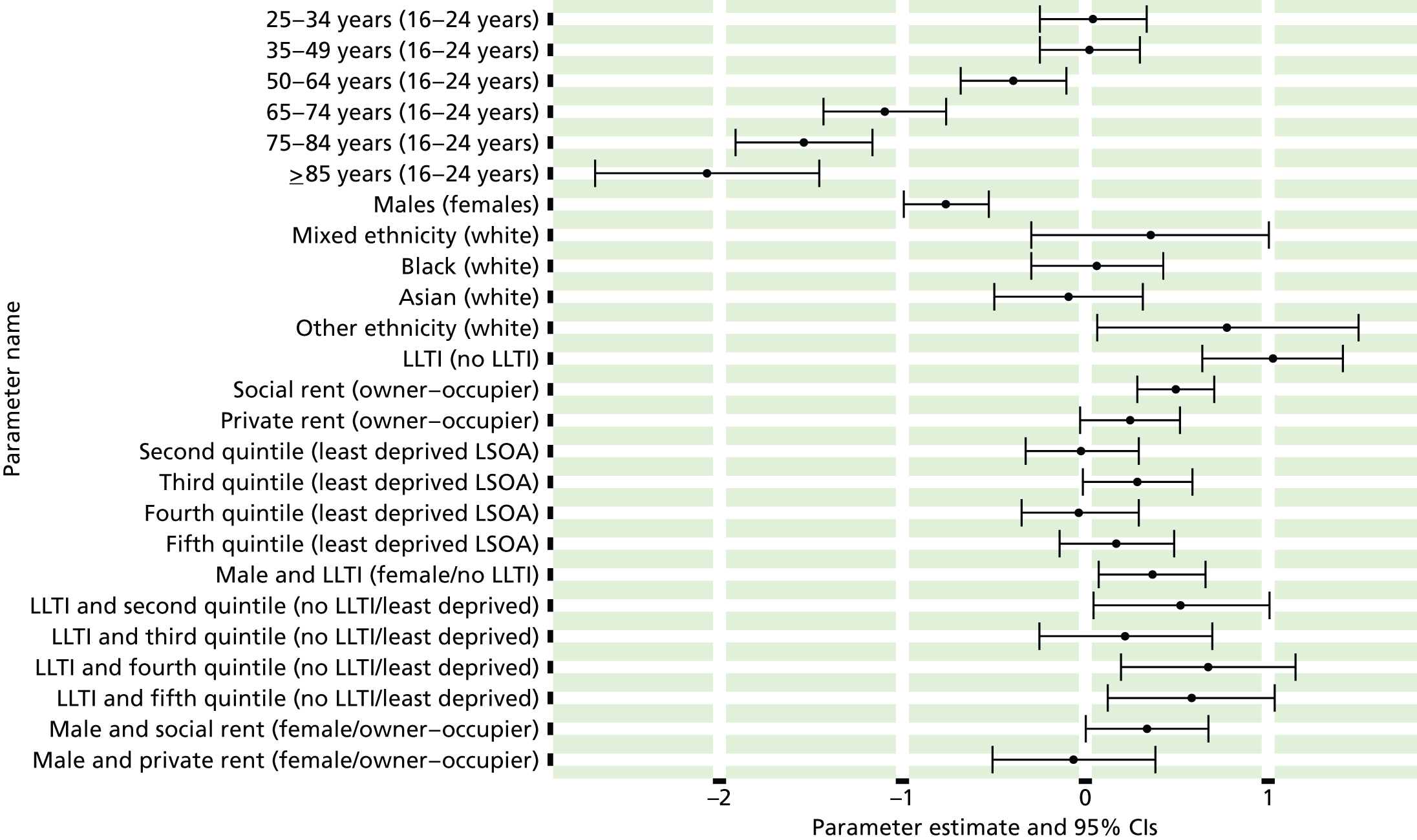
FIGURE 110.
Symptoms of generalised anxiety disorder, mixed anxiety/depressive disorder or a depressive episode: individual estimates and their 95% CIs. (a) MSOAs; (b) LAs; (c) CCGs; and (d) regions (GORs). GAD, generalised anxiety disorder; MADD, mixed anxiety/depressive disorder.
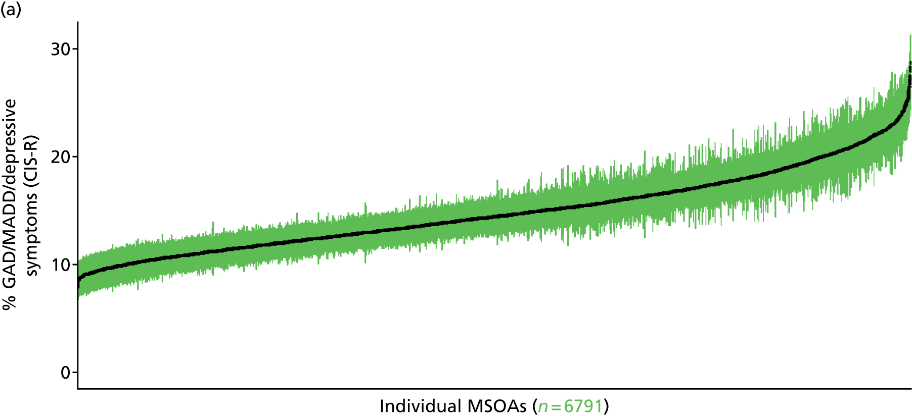
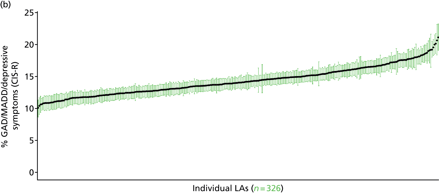
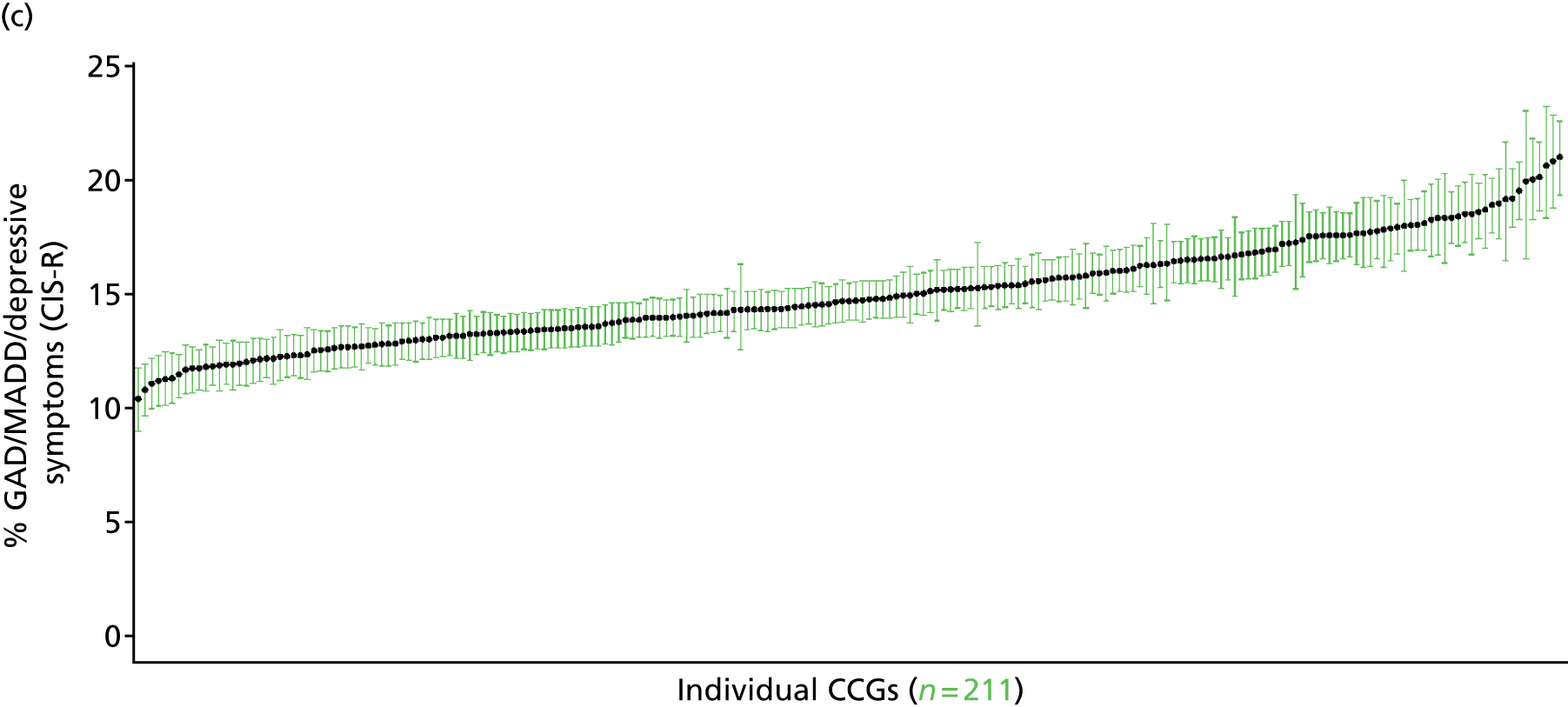
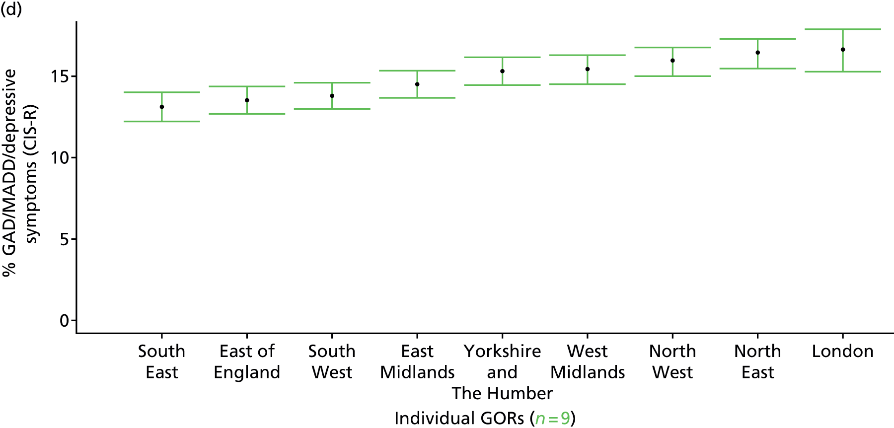
Symptoms of a neurotic disorder in past week (Adult Psychiatry Morbidity Survey, 2007)
FIGURE 111.
Symptoms of a neurotic disorder: LSOA-level map. Contains Ordnance Survey data © Crown copyright and database right 2012.
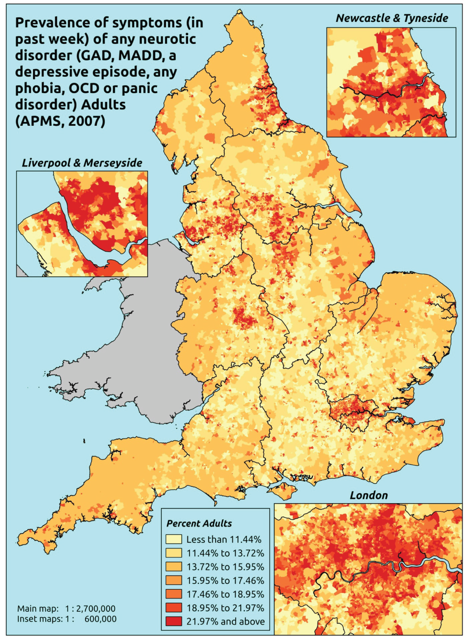
Response variable definition, provenance and prediction
On the basis of responses to the CIS-R, here we capture whether respondents to the APMS have shown symptoms of generalised anxiety disorder (ICD-10: F41.1488), mixed anxiety/depressive disorder (F41.2), a depressive episode (F32) during the previous week, or any other specified neurotic disorder (namely any phobia, an obsessive compulsive disorder or a panic disorder). This constitutes a marker for any CMHD. This is not entirely independent of sociodemographic or geographic variations in access to, or uptake of, care, as individuals may be free of symptoms because they are currently being treated for a CMHD. It may be possible to produce an alternative measure capturing underlying levels of CMHDs in that the vast majority of treatment (medication or otherwise) will be for CMHDs rather than, for instance, psychotic disorders such as schizophrenia. This marker is, however, based on symptoms only and does not include reference to treatment for a mental health disorder.
The APMS data set (n = 7403) comprises adults aged ≥ 16 years (living in England) and surveyed only one person per household; thus, the analytical data set contains all respondents for whom data is available across all model response and predictor variables, namely CIS-R question responses, age band, sex, ethnicity, LLTI, tenure and IMD quintile of LSOA of residence (n = 7326).
| Age band (years) | Females | Age band (years) | Males | ||||
|---|---|---|---|---|---|---|---|
| Does not have condition | Has condition | % | Does not have condition | Has condition | % | ||
| 16–24 | 221 | 72 | 24.6 | 16–24 | 230 | 36 | 13.5 |
| 25–34 | 469 | 145 | 23.6 | 25–34 | 343 | 64 | 15.7 |
| 35–49 | 848 | 268 | 24.0 | 35–49 | 733 | 138 | 15.8 |
| 50–64 | 807 | 206 | 20.3 | 50–64 | 688 | 109 | 13.7 |
| 65–74 | 477 | 85 | 15.1 | 65–74 | 424 | 37 | 8.0 |
| 75–84 | 383 | 52 | 12.0 | 75–84 | 268 | 18 | 6.3 |
| ≥ 85 | 120 | 13 | 9.8 | ≥ 85 | 67 | 5 | 6.9 |
| Females | 3325 | 841 | 20.2 | Males | 2753 | 407 | 12.9 |
| Total (males and females) | 6078 | 1248 | 17.0 | ||||
Model parameters are applied to microsimulated LSOA-level census data to produce estimates of the number (and proportion) of people expected to have shown symptoms of a CMHD during the previous week in each age–sex cohort (and overall) in each of the 32,844 English LSOAs. As discussed in the report, bootstrapping is used to derive 95% CIs for the estimates. These LSOA-level prevalence rate estimates (and 95% CIs) are aggregated into a number of higher geographies, namely MSOAs, LAs, CCGs and regions (GORs). Proportionate attribution is used to restructure the prevalence rate estimates to align with 2001 MSOAs, as well as GP practice populations as defined by the 2011 NHS ADS.
Table 134 summarises how expected prevalence rates vary by age, sex and local deprivation (as measured by the 2010 IMD). There are 6569 LSOAs (with 9,226,227 adults) classified as being in the least deprived quintile; 6568 LSOAs (9,525,344 adults) in the second least deprived quintile; 6568 LSOAs (9,658,444 adults) in the third least deprived quintile; 6568 LSOAs (9,650,576 adults) in the fourth least deprived quintile; and 6568 LSOAs (9,535,167 adults) in the most deprived quintile. Note that, as a general rule, variations in prevalence rates reflect variations in the socioeconomic composition of populations in the different types of LSOA rather than variations in deprivation per se.
| Cohort | Least deprived quintile LSOAs | Second least deprived quintile LSOAs | Third least deprived quintile LSOAs | Fourth least deprived quintile LSOAs | Most deprived quintile LSOAs | All England |
|---|---|---|---|---|---|---|
| Female 16–24 | 20.6 (15.4 to 25.6) | 21.5 (17.7 to 26.2) | 26.5 (21.9 to 31.5) | 21.7 (17.9 to 27.1) | 25.1 (21.3 to 30.6) | 23.3 (20.1 to 27.5) |
| Female 25–34 | 16.5 (12.9 to 19.2) | 18.5 (15.4 to 21.8) | 24.0 (19.9 to 27.6) | 21.4 (18.3 to 25.1) | 27.0 (23.8 to 30.6) | 22.2 (19.8 to 24.9) |
| Female 35–49 | 17.3 (13.9 to 19.9) | 20.0 (17.2 to 23.0) | 26.0 (22.8 to 28.9) | 24.8 (21.9 to 28.3) | 31.6 (28.4 to 34.9) | 23.9 (21.9 to 26.1) |
| Female 50–64 | 13.6 (10.9 to 15.7) | 17.5 (15.3 to 20.1) | 22.0 (18.5 to 24.9) | 23.0 (20.1 to 26.3) | 30.0 (27.4 to 33.7) | 20.8 (18.4 to 23.0) |
| Female 65–74 | 8.8 (6.4 to 10.6) | 12.5 (9.7 to 15.3) | 15.1 (11.7 to 18.2) | 16.5 (12.9 to 19.9) | 21.2 (16.7 to 25.4) | 14.4 (11.6 to 16.7) |
| Female ≥ 75 | 8.3 (5.7 to 10.6) | 12.5 (9.3 to 15.6) | 13.8 (9.9 to 17.4) | 14.4 (10.3 to 18.8) | 16.1 (12.2 to 20.5) | 12.9 (9.7 to 15.6) |
| Females | 14.2 (11.1 to 16.8) | 17.3 (14.5 to 20.4) | 21.9 (18.2 to 25.2) | 21.3 (18.0 to 25.1) | 26.8 (23.4 to 30.7) | 20.3 (17.8 to 22.9) |
| Male 16–24 | 11.6 (8.4 to 15.3) | 12.6 (10.4 to 16.1) | 16.2 (13.6 to 20.1) | 13.8 (11.2 to 17.1) | 17.1 (14.1 to 21.0) | 14.5 (12.1 to 17.6) |
| Male 25–34 | 9.5 (7.1 to 11.2) | 11.0 (8.9 to 13.0) | 14.8 (12.0 to 17.7) | 13.7 (11.7 to 15.7) | 18.7 (15.9 to 21.9) | 14.2 (12.2 to 16.0) |
| Male 35–49 | 9.6 (7.4 to 11.1) | 11.8 (10.2 to 13.6) | 16.0 (13.7 to 18.5) | 16.2 (14.1 to 18.5) | 22.7 (20.0 to 25.3) | 15.3 (13.7 to 16.9) |
| Male 50–64 | 7.6 (6.1 to 9.0) | 10.5 (9.1 to 12.2) | 13.7 (11.6 to 16.0) | 15.3 (13.5 to 18.0) | 21.4 (18.9 to 24.8) | 13.4 (12.1 to 15.1) |
| Male 65–74 | 5.1 (3.5 to 6.2) | 7.8 (5.6 to 9.7) | 9.6 (7.3 to 12.0) | 11.0 (8.6 to 13.6) | 15.2 (11.4 to 18.9) | 9.3 (7.3 to 11.1) |
| Male ≥ 75 | 4.9 (3.4 to 6.6) | 7.5 (5.6 to 9.9) | 8.5 (6.4 to 11.2) | 9.1 (6.5 to 12.0) | 10.8 (8.4 to 14.5) | 7.9 (6.2 to 10.1) |
| Males | 8.2 (6.2 to 9.9) | 10.5 (8.7 to 12.5) | 13.8 (11.4 to 16.4) | 14.1 (11.9 to 16.6) | 19.2 (16.4 to 22.4) | 13.2 (11.4 to 15.1) |
| All | 11.3 (9.4 to 12.7) | 14.0 (12.5 to 15.5) | 18.0 (16.1 to 19.6) | 17.8 (16.1 to 19.7) | 23.1 (21.2 to 24.9) | 16.9 (16.1 to 17.6) |
| Factor (reference group) | Model coefficients | 95% CI | ||
|---|---|---|---|---|
| Estimate | SE | 2.5% CI | 97.5% | |
| (Intercept) | –1.45269 | 0.20596 | –1.85637 | –1.04901 |
| Age (16–24 years) | ||||
| 25–34 years | –0.48952 | 0.21306 | –0.90713 | –0.07192 |
| 35–49 years | –0.47358 | 0.18982 | –0.84564 | –0.10153 |
| 50–64 years | –0.86062 | 0.19375 | –1.24037 | –0.48088 |
| 65–74 years | –1.56366 | 0.21936 | –1.99360 | –1.13371 |
| 75–84 years | –1.87658 | 0.23894 | –2.34490 | –1.40825 |
| ≥ 85 years | –2.03222 | 0.35047 | –2.71914 | –1.34531 |
| Sex (females) | ||||
| Males | –0.76062 | 0.11551 | –0.98703 | –0.53421 |
| Ethnicity (white) | ||||
| Mixed | 0.34638 | 0.32621 | –0.29299 | 0.98575 |
| Black | 0.09660 | 0.17929 | –0.25481 | 0.44800 |
| Asian | –0.19993 | 0.20544 | –0.60259 | 0.20273 |
| Other | 0.63691 | 0.36758 | –0.08355 | 1.35737 |
| LLTI (no LTTI) | ||||
| LLTI | 1.21024 | 0.18935 | 0.83911 | 1.58137 |
| Tenure (owner–occupier) | ||||
| Social rent | 0.03461 | 0.27482 | –0.50405 | 0.57326 |
| Private rent or other tenure | –0.30152 | 0.29663 | –0.88291 | 0.27987 |
| LSOA deprivation quintile (least deprived quintile) | ||||
| Second LSOA deprivation quintile | –0.00278 | 0.15267 | –0.30200 | 0.29645 |
| Third LSOA deprivation quintile | 0.31646 | 0.15053 | 0.02143 | 0.61150 |
| Fourth LSOA deprivation quintile | –0.03221 | 0.15931 | –0.34447 | 0.28004 |
| Fifth LSOA deprivation quintile ( = most deprived) | 0.13829 | 0.15643 | –0.16831 | 0.44489 |
| Interaction effects | ||||
| Male and social rent | 0.42067 | 0.16835 | 0.09070 | 0.75063 |
| Male and private rent or other tenure | –0.05181 | 0.22044 | –0.48386 | 0.38025 |
| LLTI and second LSOA deprivation quintile | 0.50121 | 0.23743 | 0.03584 | 0.96657 |
| LLTI and second LSOA deprivation quintile | 0.26182 | 0.23279 | –0.19445 | 0.71809 |
| LLTI and second LSOA deprivation quintile | 0.66811 | 0.23749 | 0.20263 | 1.13359 |
| LLTI and second LSOA deprivation quintile | 0.62057 | 0.22874 | 0.17224 | 1.06890 |
| 25–34 years and social rent | 0.92242 | 0.33507 | 0.26568 | 1.57916 |
| 35–49 years and social rent | 0.66148 | 0.30404 | 0.06556 | 1.25741 |
| 50–64 years and social rent | 0.41681 | 0.31226 | –0.19522 | 1.02885 |
| 65–74 years and social rent | 0.40076 | 0.34758 | –0.28049 | 1.08202 |
| 75–84 years and social rent | –0.34928 | 0.40428 | –1.14167 | 0.44311 |
| ≥ 85 years and social rent | –0.74275 | 0.65824 | –2.03290 | 0.54739 |
| 25–34 years and private rent or other tenure | 0.78694 | 0.35550 | 0.09016 | 1.48371 |
| 35–49 years and private rent or other tenure | 0.88701 | 0.34167 | 0.21734 | 1.55668 |
| 50–64 years and private rent or other tenure | 0.58867 | 0.39786 | –0.19114 | 1.36848 |
| 65–74 years and private rent or other tenure | 0.15348 | 0.57895 | –0.98127 | 1.28823 |
| 75–84 years and private rent or other tenure | 0.52744 | 0.64311 | –0.73306 | 1.78795 |
| ≥ 85 years and private rent or other tenure | 0.22714 | 1.13786 | –2.00307 | 2.45735 |
| Male and LLTI | 0.20378 | 0.14535 | –0.08110 | 0.48867 |
FIGURE 112.
Parameter plots: symptoms of a neurotic disorder.

FIGURE 113.
Symptoms of a neurotic disorder: individual estimates and their 95% CIs. (a) MSOAs; (b) LAs; (c) CCGs; and (d) regions (GORs).

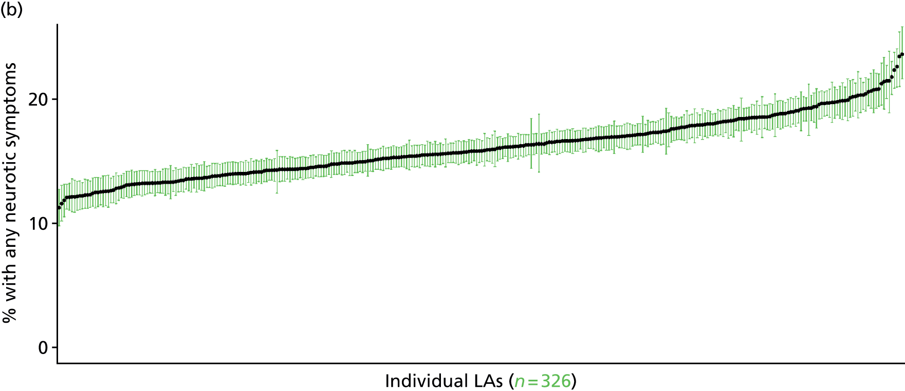
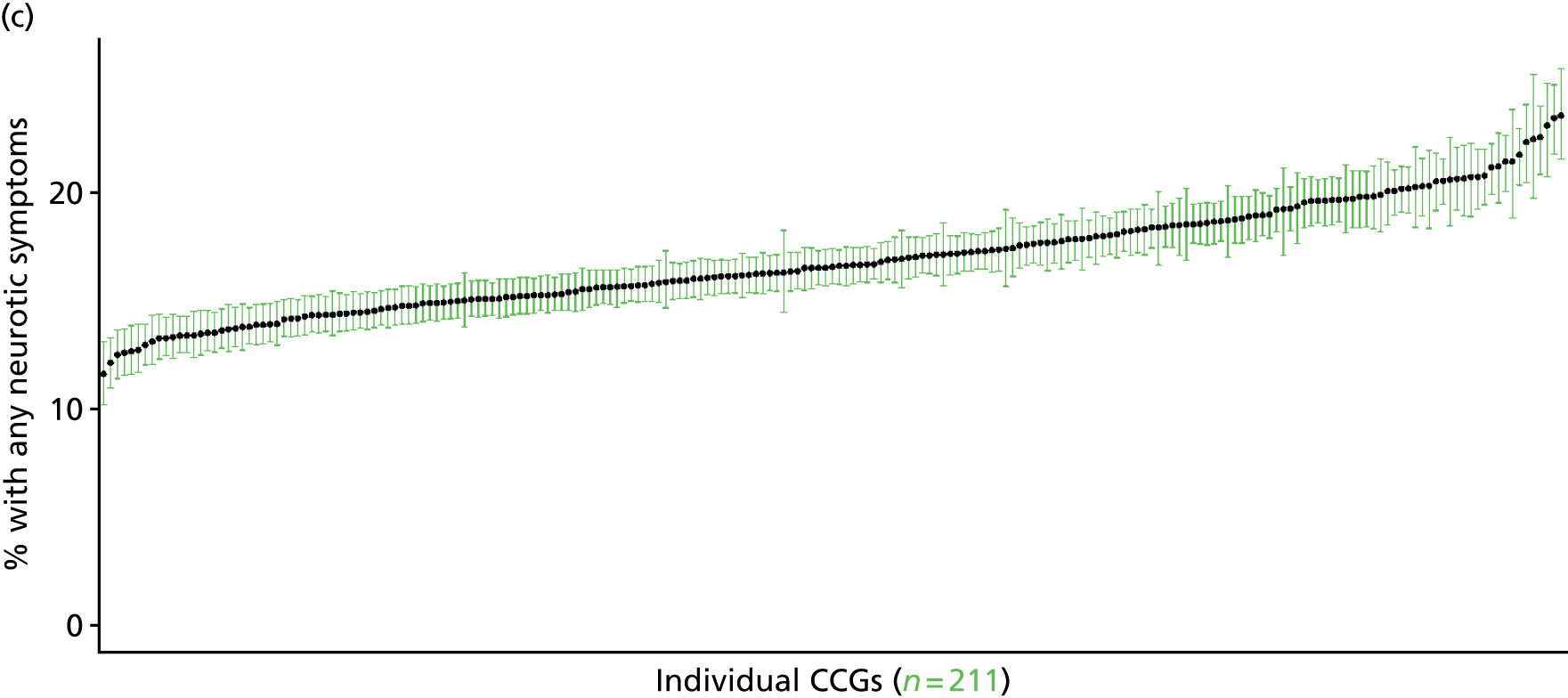
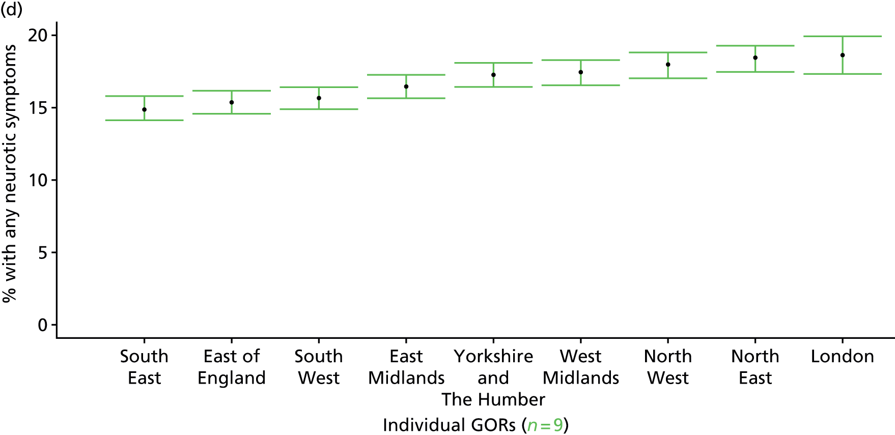
‘Possible’ psychiatric morbidity (12-item General Health Questionnaire score of ≥ 4) (Health Survey for England, 2006 and 2008–10)
FIGURE 114.
‘Possible’ psychiatric morbidity (HSfE GHQ12 score of ≥ 4): LSOA-level map. Contains Ordnance Survey data © Crown copyright and database right 2012.
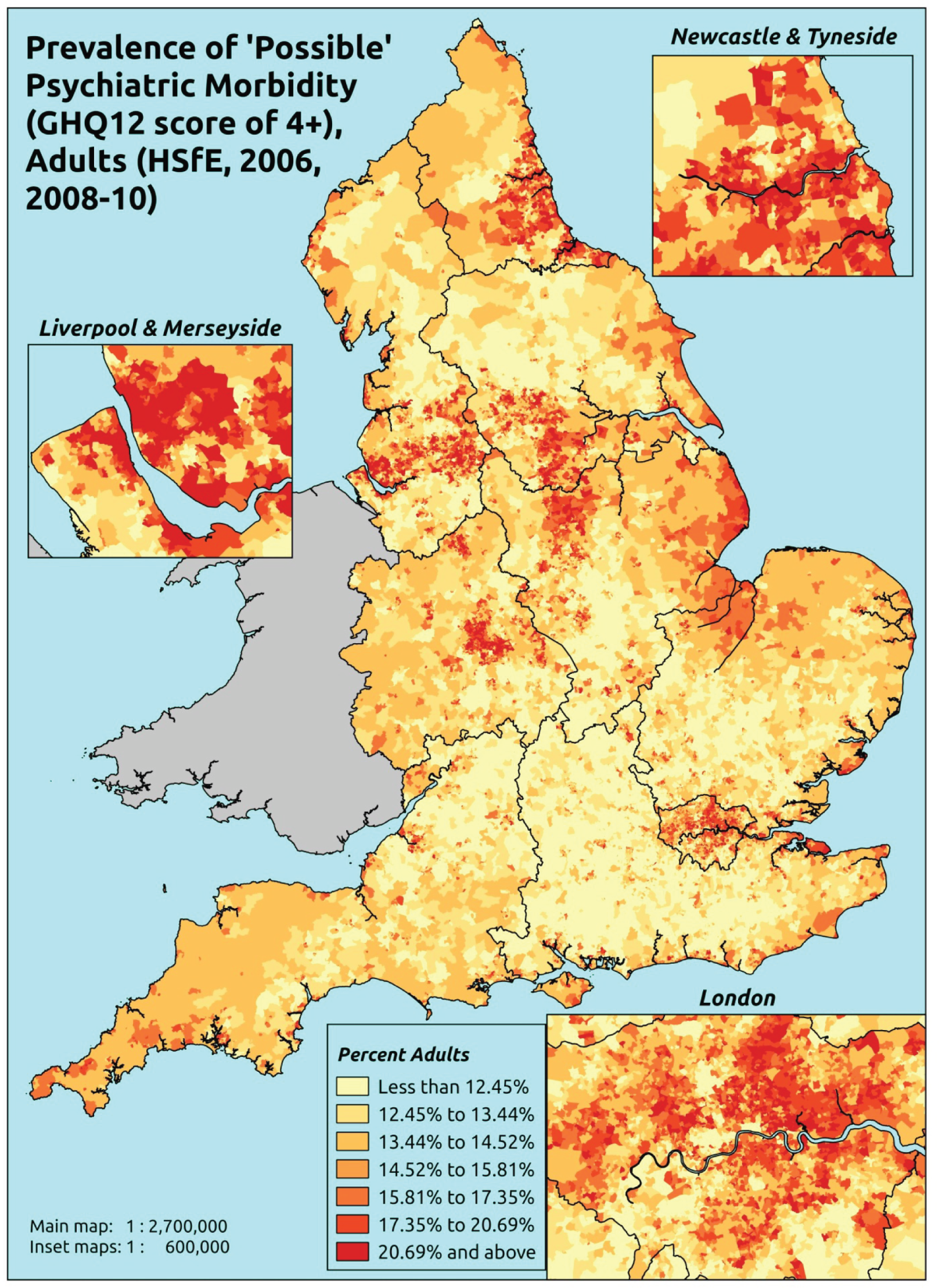
Response variable definition, provenance and prediction
Based on the GHQ12 incorporated within the HSfE in 2006 and 2008–10, here we capture whether people score ≥ 4 using the standard 0–12 ‘caseness’ scoring approach. The GHQ12 is a screening device for identifying minor psychiatric disorders in the general population. It assesses the respondent’s current state and asks if that differs from their usual state. It is sensitive to short-term psychiatric disorders but not long-standing attributes of the respondent. In the literature a score of ≥ 4 is usually taken as being indicative of ‘possible psychiatric morbidity’. This marker of mental health needs is not independent of sociodemographic or geographic variations in access to, or uptake of, care as individuals may score < 4 because they are currently being treated for a mental health issue. (See below for an alternative marker below which includes people currently being treated with medication for anxiety/depression.)
The HSfE at this time includes multiple household respondents of all ages. The analytical data set is drawn from a subset of respondents aged ≥ 16 years for whom data are available across all model response and predictor variables, namely whether or not they completed the GHQ12 questionnaire, along with information on age band, sex, ethnicity, general health status, LLTI, tenure and the IMD quintile of the LSOA of residence (n = 38,935). A single randomly selected adult is then drawn from each household, resulting in an analytical data set of 23,390 adults aged ≥ 16 years.
| Age band (years) | Females | Age band (years) | Males | ||||
|---|---|---|---|---|---|---|---|
| Does not have condition | Has condition | % | Does not have condition | Has condition | % | ||
| 16–24 | 860 | 168 | 16.3 | 16–24 | 634 | 78 | 11.0 |
| 25–34 | 1644 | 326 | 16.5 | 25–34 | 1082 | 171 | 13.6 |
| 35–49 | 2944 | 586 | 16.6 | 35–49 | 2130 | 359 | 14.4 |
| 50–64 | 2577 | 516 | 16.7 | 50–64 | 2108 | 377 | 15.2 |
| 65–74 | 1443 | 229 | 13.7 | 65–74 | 1235 | 142 | 10.3 |
| 75–84 | 1087 | 192 | 15.0 | 75–84 | 720 | 103 | 12.5 |
| ≥ 85 | 385 | 78 | 16.8 | ≥ 85 | 172 | 44 | 20.4 |
| Females | 10,940 | 2095 | 16.1 | Males | 8081 | 1274 | 13.6 |
| Total (males and females) | 19,021 | 3369 | 15.0 | ||||
Model parameters are applied to microsimulated LSOA-level census data to produce estimates of the number (and proportion) of people with ‘possible psychiatric morbidity (i.e. who would score ≥ 4 on the GHQ12) in each age–sex cohort (and overall) in each of the 32,844 English LSOAs. As discussed in the report, bootstrapping is used to derive 95% CIs for the estimates. These LSOA-level prevalence rate estimates (and 95% CIs) are aggregated into a number of higher geographies; namely MSOAs, LAs, CCGs and regions (GORs). Proportionate attribution is used to restructure the prevalence rate estimates to align with 2001 MSOAs, as well as GP practice populations as defined by the 2011 NHS ADS.
Table 137 summarises how expected prevalence rates vary by age, sex and local deprivation (as measured by the 2010 IMD). There are 6569 LSOAs (with 9,226,227 adults) classified as being in the least deprived quintile; 6568 LSOAs (9,525,344 adults) in the second least deprived quintile; 6568 LSOAs (9,658,444 adults) in the third least deprived quintile; 6568 LSOAs (9,650,576 adults) in the fourth least deprived quintile; and 6568 LSOAs (9,535,167 adults) in the most deprived quintile. Note that, as a general rule, variations in prevalence rates reflect variations in the socioeconomic composition of populations in the different types of LSOA rather than variations in deprivation per se.
| Cohort | Least deprived quintile LSOAs | Second least deprived quintile LSOAs | Third least deprived quintile LSOAs | Fourth least deprived quintile LSOAs | Most deprived quintile LSOAs | All England |
|---|---|---|---|---|---|---|
| Female 16–24 | 11.6 (9.8 to 12.8) | 11.6 (10.0 to 13.1) | 12.7 (11.1 to 14.1) | 13.2 (11.3 to 14.5) | 15.8 (13.9 to 17.1) | 13.2 (11.7 to 14.5) |
| Female 25–34 | 11.7 (10.6 to 13.0) | 11.9 (10.9 to 13.1) | 13.5 (12.4 to 14.7) | 14.5 (13.2 to 15.8) | 18.5 (17.0 to 19.9) | 14.5 (13.4 to 15.5) |
| Female 35–49 | 13.3 (12.3 to 14.4) | 14.2 (13.2 to 15.2) | 16.8 (15.5 to 17.7) | 19.1 (17.7 to 20.2) | 25.2 (23.6 to 26.4) | 17.7 (16.8 to 18.4) |
| Female 50–64 | 14.0 (12.9 to 15.3) | 15.4 (14.3 to 17.0) | 18.4 (17.1 to 19.8) | 21.7 (20.4 to 23.1) | 29.5 (27.8 to 31.2) | 19.3 (18.5 to 20.5) |
| Female 65–74 | 12.4 (11.3 to 13.9) | 13.6 (12.6 to 15.1) | 16.1 (14.5 to 17.5) | 18.8 (17.1 to 20.5) | 25.2 (23.2 to 27.6) | 16.7 (15.5 to 18.1) |
| Female ≥ 75 | 19.9 (18.0 to 21.8) | 20.3 (18.6 to 22.6) | 22.3 (20.3 to 24.4) | 23.3 (20.9 to 25.7) | 27.7 (24.6 to 30.0) | 22.4 (20.4 to 24.3) |
| Females | 13.9 (12.7 to 15.3) | 14.7 (13.5 to 16.2) | 16.8 (15.4 to 18.2) | 18.5 (16.9 to 19.9) | 23.5 (21.7 to 25.1) | 17.5 (16.3 to 18.6) |
| Male 16–24 | 8.9 (7.6 to 10.0) | 9.0 (7.8 to 10.3) | 10.2 (8.8 to 11.5) | 10.8 (9.3 to 11.9) | 13.5 (11.7 to 14.6) | 10.7 (9.4 to 11.8) |
| Male 25–34 | 9.4 (8.6 to 10.5) | 9.8 (8.8 to 10.9) | 11.1 (10.1 to 12.2) | 12.1 (11.0 to 13.3) | 16.0 (14.8 to 17.4) | 12.1 (11.3 to 13.2) |
| Male 35–49 | 10.3 (9.5 to 11.3) | 11.3 (10.4 to 12.3) | 13.6 (12.5 to 14.7) | 15.8 (14.6 to 16.8) | 21.9 (20.5 to 23.2) | 14.6 (13.9 to 15.3) |
| Male 50–64 | 11.3 (10.5 to 12.5) | 12.8 (11.8 to 14.1) | 15.6 (14.6 to 17.0) | 18.9 (17.8 to 20.3) | 26.4 (24.7 to 28.2) | 16.6 (15.8 to 17.7) |
| Male 65–74 | 10.2 (9.3 to 11.4) | 11.3 (10.5 to 12.8) | 13.8 (12.4 to 15.0) | 16.3 (14.8 to 18.0) | 22.5 (20.5 to 24.5) | 14.3 (13.2 to 15.6) |
| Male ≥ 75 | 15.3 (13.8 to 17.1) | 16.0 (14.6 to 17.8) | 17.7 (16.1 to 19.7) | 18.9 (16.7 to 20.8) | 23.2 (20.4 to 25.6) | 17.8 (16.2 to 19.4) |
| Males | 10.9 (9.9 to 12.0) | 11.7 (10.7 to 13.0) | 13.7 (12.5 to 15.0) | 15.3 (14.0 to 16.6) | 20.4 (18.7 to 21.9) | 14.4 (13.5 to 15.5) |
| All | 12.4 (11.7 to 13.3) | 13.3 (12.6 to 14.3) | 15.3 (14.5 to 16.2) | 16.9 (16.0 to 17.8) | 22.0 (20.8 to 22.8) | 16.0 (15.6 to 16.4) |
| Factor (reference group) | Model coefficients | 95% CI | ||
|---|---|---|---|---|
| Estimate | SE | 2.5% CI | 97.50% | |
| (Intercept) | –2.48556 | 0.12767 | –2.73579 | –2.23534 |
| Age (16–24 years) | ||||
| 25–34 years | –0.11176 | 0.13737 | –0.38101 | 0.15749 |
| 35–49 years | –0.11463 | 0.12267 | –0.35506 | 0.12581 |
| 50–64 years | –0.41196 | 0.12389 | –0.65479 | –0.16914 |
| 65–74 years | –0.9332 | 0.13628 | –1.2003 | –0.6661 |
| 75–84 years | –0.83596 | 0.14175 | –1.11378 | –0.55814 |
| ≥ 85 years | –0.46094 | 0.17559 | –0.80509 | –0.11679 |
| Sex (females) | ||||
| Males | –0.2689 | 0.05297 | –0.37272 | –0.16509 |
| Ethnicity (white) | ||||
| Mixed | 0.39098 | 0.18128 | 0.03566 | 0.74629 |
| Black | 0.05355 | 0.09759 | –0.13772 | 0.24482 |
| Asian | –0.08612 | 0.13295 | –0.3467 | 0.17447 |
| Other | –0.019 | 0.2893 | –0.58603 | 0.54802 |
| General health status (very good health) | ||||
| Good health | 0.50141 | 0.06017 | 0.38348 | 0.61934 |
| Fair health | 1.32364 | 0.06823 | 1.18991 | 1.45737 |
| Bad health | 2.31198 | 0.0883 | 2.13891 | 2.48505 |
| Very bad health | 2.9897 | 0.12999 | 2.73492 | 3.24448 |
| LLTI (no LTTI) | ||||
| LLTI | 0.70989 | 0.05161 | 0.60873 | 0.81105 |
| Tenure (owner–occupier) | ||||
| Social rent | 0.0981 | 0.18045 | –0.2556 | 0.45179 |
| Private rent or other tenure | 0.16079 | 0.17637 | –0.18489 | 0.50648 |
| LSOA deprivation quintile (least deprived quintile) | ||||
| Second LSOA deprivation quintile | –0.03605 | 0.06807 | –0.16946 | 0.09737 |
| Third LSOA deprivation quintile | 0.03732 | 0.06698 | –0.09396 | 0.16859 |
| Fourth LSOA deprivation quintile | 0.02369 | 0.06754 | –0.10869 | 0.15607 |
| Fifth LSOA deprivation quintile ( = most deprived) | 0.1786 | 0.06963 | 0.04213 | 0.31507 |
| Interaction effects | ||||
| 25–34 years and social rent | 0.28617 | 0.21877 | –0.14262 | 0.71496 |
| 35–49 years and social rent | 0.14432 | 0.20102 | –0.24968 | 0.53832 |
| 50–64 years and social rent | –0.05315 | 0.20389 | –0.45277 | 0.34648 |
| 65–74 years and social rent | –0.11082 | 0.22615 | –0.55407 | 0.33243 |
| 75–84 years and social rent | –0.37465 | 0.23569 | –0.8366 | 0.0873 |
| ≥ 85 years and social rent | –0.58592 | 0.29418 | –1.16251 | –0.00932 |
| 25–34 years and private rent or other tenure | 0.27209 | 0.21027 | –0.14004 | 0.68423 |
| 35–49 years and private rent or other tenure | 0.19335 | 0.20442 | –0.20731 | 0.59401 |
| 50–64 years and private rent or other tenure | 0.23916 | 0.23128 | –0.21414 | 0.69246 |
| 65–74 years and private rent or other tenure | 0.36603 | 0.31734 | –0.25595 | 0.98802 |
| 75–84 years and private rent or other tenure | –0.84007 | 0.41381 | –1.65114 | –0.02899 |
| ≥ 85 years and private rent or other tenure | –1.42118 | 0.79512 | –2.97961 | 0.13725 |
| Male and social rent | 0.21163 | 0.1035 | 0.00877 | 0.4145 |
| Male and private rent or other tenure | 0.03568 | 0.12274 | –0.20489 | 0.27626 |
FIGURE 115.
Parameter plots: ‘possible’ psychiatric morbidity (HSfE GHQ12 score of ≥ 4).
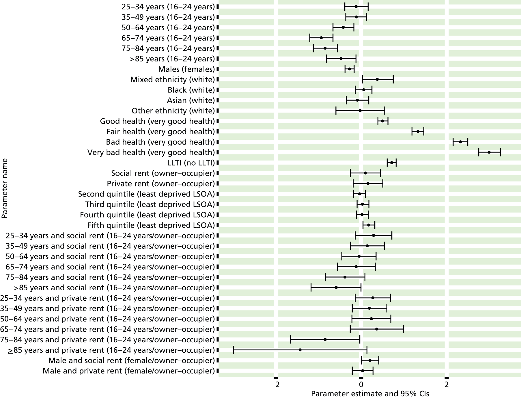
FIGURE 116.
‘Possible’ psychiatric morbidity (HSfE GHQ12 score of ≥ 4): individual estimates and their 95% CIs. (a) MSOAs; (b) LAs; (c) CCGs; and (d) regions (GORs).
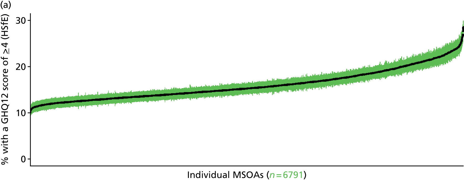
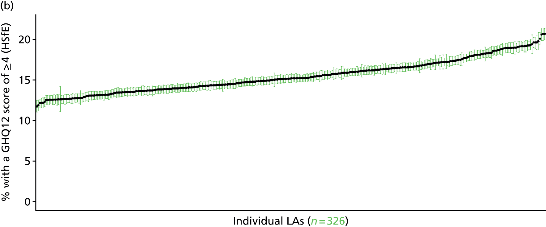
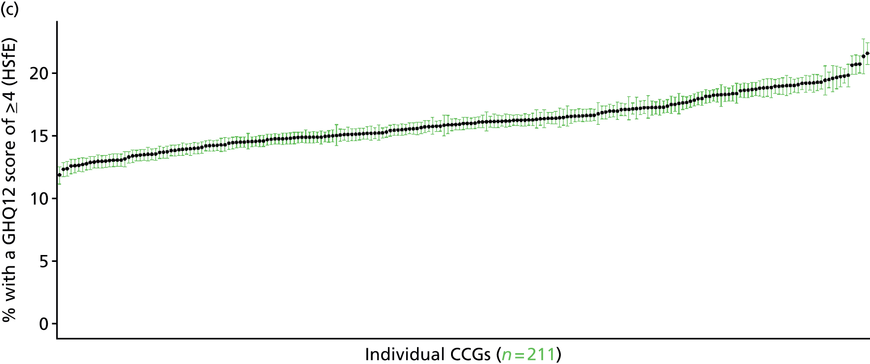

‘Probable’ psychiatric morbidity (12-item General Health Questionnaire score of ≥ 6) (Health Survey for England, 2006 and 2008–10)
FIGURE 117.
‘Probable’ psychiatric morbidity (HSfE GHQ12 of ≥ 6): LSOA-level map. Contains Ordnance Survey data © Crown copyright and database right 2012.
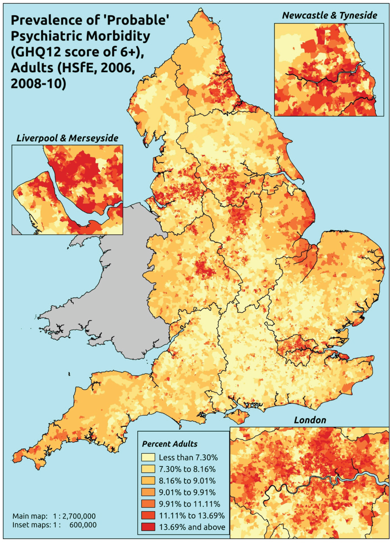
Response variable definition, provenance and prediction
Based on the GHQ12 incorporated within the HSfE in 2006 and 2008–10, here we capture whether people score 6 or more using the standard 0–12 ‘caseness’ scoring approach. The GHQ12 is a screening device for identifying minor psychiatric disorders in the general population. It assesses the respondent’s current state and asks if that differs from their usual state. It is sensitive to short-term psychiatric disorders but not long-standing attributes of the respondent. In the literature a score of ≥ 4 is usually taken as being indicative of ‘possible psychiatric morbidity’, but occasionally a ≥ 6 threshold is used. For convenience (and without clinical justification) we describe this as a marker of ‘probable psychiatric morbidity’ – to distinguish this marker from those using the standard ≥ 4 threshold (‘possible psychiatric morbidity’) and the higher ≥ 8 threshold (‘psychiatric morbidity’). This is not independent of sociodemographic or geographic variations in access to, or uptake of, care as individuals may score below 6 because they are currently being treated for a mental health issue. (See below for an alternative marker below which includes people currently being treated with medication for anxiety/depression.)
The HSfE at this time includes multiple household respondents of all ages. The analytical data set is drawn from a subset of respondents aged ≥ 16 years for whom data are available across all model response and predictor variables, namely whether or not they completed the GHQ12 questionnaire, along with information on age band, sex, ethnicity, general health status, LLTI, tenure and the IMD quintile of the LSOA of residence (n = 38,935). A single randomly selected adult is then drawn from each household, resulting in an analytical data set of 23,390 adults aged ≥ 16 years.
| Age band (years) | Females | Age band (years) | Males | ||||
|---|---|---|---|---|---|---|---|
| Does not have condition | Has condition | % | Does not have condition | Has condition | % | ||
| 16–24 | 930 | 98 | 9.5 | 16–24 | 678 | 34 | 4.8 |
| 25–34 | 1761 | 209 | 10.6 | 25–34 | 1157 | 96 | 7.7 |
| 35–49 | 3147 | 383 | 10.8 | 35–49 | 2242 | 247 | 9.9 |
| 50–64 | 2749 | 344 | 11.1 | 50–64 | 2224 | 261 | 10.5 |
| 65–74 | 1546 | 126 | 7.5 | 65–74 | 1284 | 93 | 6.8 |
| 75–84 | 1171 | 108 | 8.4 | 75–84 | 760 | 63 | 7.7 |
| ≥ 85 | 419 | 44 | 9.5 | ≥ 85 | 192 | 24 | 11.1 |
| Females | 11,723 | 1312 | 10.1 | Males | 8537 | 818 | 8.7 |
| Total (males and females) | 20,260 | 2130 | 9.5 | ||||
Model parameters are applied to microsimulated LSOA-level census data to produce estimates of the number (and proportion) of people with ‘probable’ psychiatric morbidity (i.e. who would score ≥ 6 on the GHQ12) in each age–sex cohort (and overall) in each of the 32,844 English LSOAs. As discussed in the report, bootstrapping is used to derive 95% CIs for the estimates. These LSOA-level prevalence rate estimates (and 95% CIs) are aggregated into a number of higher geographies, namely MSOAs, LAs, CCGs and regions (GORs). Proportionate attribution is used to restructure the prevalence rate estimates to align with 2001 MSOAs, as well as GP practice populations as defined by the 2011 NHS ADS.
Table 140 summarises how expected prevalence rates vary by age, sex and local deprivation (as measured by the 2010 IMD). There are 6569 LSOAs (with 9,226,227 adults) classified as being in the least deprived quintile; 6568 LSOAs (9,525,344 adults) in the second least deprived quintile; 6568 LSOAs (9,658,444 adults) in the third least deprived quintile; 6568 LSOAs (9,650,576 adults) in the fourth least deprived quintile; and 6568 LSOAs (9,535,167 adults) in the most deprived quintile. Note that, as a general rule, variations in prevalence rates reflect variations in the socioeconomic composition of populations in the different types of LSOA rather than variations in deprivation per se.
| Cohort | Least deprived quintile LSOAs | Second least deprived quintile LSOAs | Third least deprived quintile LSOAs | Fourth least deprived quintile LSOAs | Most deprived quintile LSOAs | All England |
|---|---|---|---|---|---|---|
| Female 16–24 | 5.4 (4.5 to 6.3) | 6.0 (5.0 to 6.8) | 6.5 (5.5 to 7.5) | 6.9 (5.9 to 7.9) | 8.7 (7.5 to 9.7) | 6.9 (6.0 to 7.7) |
| Female 25–34 | 6.8 (6.0 to 7.7) | 7.4 (6.7 to 8.4) | 8.2 (7.4 to 9.4) | 8.9 (8.1 to 10.0) | 11.6 (10.6 to 12.8) | 8.9 (8.3 to 9.7) |
| Female 35–49 | 8.2 (7.4 to 9.0) | 9.5 (8.6 to 10.5) | 11.1 (10.3 to 12.3) | 13.1 (12.0 to 14.3) | 17.9 (16.7 to 19.0) | 11.9 (11.3 to 12.7) |
| Female 50–64 | 8.4 (7.6 to 9.4) | 10.0 (9.1 to 11.3) | 12.0 (11.0 to 13.6) | 14.7 (13.5 to 16.2) | 21.0 (19.4 to 22.9) | 12.9 (12.1 to 13.9) |
| Female 65–74 | 6.4 (5.6 to 7.5) | 7.6 (6.8 to 8.7) | 8.8 (8.0 to 10.3) | 10.7 (9.4 to 12.3) | 15.2 (13.9 to 17.5) | 9.4 (8.6 to 10.6) |
| Female ≥ 75 | 10.4 (9.1 to 11.8) | 11.7 (10.6 to 13.4) | 12.9 (11.5 to 14.8) | 14.4 (12.9 to 16.0) | 18.3 (16.4 to 20.5) | 13.3 (12.1 to 14.6) |
| Females | 7.9 (7.0 to 8.9) | 9.0 (8.1 to 10.2) | 10.3 (9.3 to 11.7) | 11.7 (10.6 to 13.0) | 15.6 (14.3 to 17.1) | 10.9 (10.1 to 11.9) |
| Male 16–24 | 4.2 (3.4 to 4.9) | 4.5 (3.8 to 5.5) | 5.1 (4.3 to 5.8) | 5.5 (4.6 to 6.3) | 7.0 (6.1 to 8.1) | 5.4 (4.7 to 6.1) |
| Male 25–34 | 5.4 (4.8 to 6.2) | 6.0 (5.3 to 6.8) | 6.5 (5.9 to 7.4) | 7.2 (6.5 to 8.2) | 9.8 (8.9 to 10.8) | 7.3 (6.7 to 8.0) |
| Male 35–49 | 6.4 (5.6 to 7.0) | 7.6 (6.8 to 8.4) | 9.0 (8.1 to 9.9) | 10.8 (9.7 to 11.7) | 15.5 (14.2 to 16.4) | 9.9 (9.1 to 10.5) |
| Male 50–64 | 7.1 (6.4 to 7.9) | 8.7 (7.9 to 9.8) | 10.7 (9.7 to 11.9) | 13.2 (12.0 to 14.6) | 19.3 (17.9 to 21.0) | 11.5 (10.7 to 12.4) |
| Male 65–74 | 5.7 (4.9 to 6.6) | 6.8 (6.2 to 8.1) | 8.1 (7.3 to 9.5) | 9.9 (8.7 to 11.3) | 14.1 (12.7 to 16.1) | 8.6 (7.8 to 9.8) |
| Male ≥ 75 | 8.8 (7.7 to 9.9) | 10.0 (8.7 to 11.4) | 11.1 (9.9 to 12.8) | 12.4 (10.9 to 14.1) | 16.1 (14.2 to 18.0) | 11.3 (10.1 to 12.7) |
| Males | 6.4 (5.6 to 7.2) | 7.4 (6.6 to 8.5) | 8.6 (7.7 to 9.7) | 9.9 (8.8 to 11.0) | 13.6 (12.4 to 14.9) | 9.2 (8.4 to 10.1) |
| All | 7.2 (6.6 to 7.8) | 8.3 (7.7 to 9.0) | 9.5 (8.9 to 10.3) | 10.8 (10.1 to 11.6) | 14.7 (13.9 to 15.5) | 10.1 (9.8 to 10.5) |
| Factor (reference group) | Model coefficients | 95% CI | ||
|---|---|---|---|---|
| Estimate | SE | 2.5% CI | 97.50% | |
| (Intercept) | –3.49429 | 0.13239 | –3.75377 | –3.23481 |
| Age (16–24 years) | ||||
| 25–34 years | 0.17090 | 0.11390 | –0.05234 | 0.39414 |
| 35–49 years | 0.17401 | 0.10708 | –0.03587 | 0.38390 |
| 50–64 years | –0.19492 | 0.11144 | –0.41335 | 0.02351 |
| 65–74 years | –0.87139 | 0.12727 | –1.12084 | –0.62194 |
| 75–84 years | –0.9296 | 0.13381 | –1.19187 | –0.66733 |
| ≥ 85 years | –0.73051 | 0.17078 | –1.06524 | –0.39578 |
| Sex (females) | ||||
| Males | –0.27103 | 0.07338 | –0.41484 | –0.12721 |
| Ethnicity (white) | ||||
| Mixed | 0.53173 | 0.20740 | 0.12523 | 0.93823 |
| Black | 0.20294 | 0.11223 | –0.01703 | 0.42291 |
| Asian | –0.16587 | 0.16641 | –0.49204 | 0.16029 |
| Other | –0.30466 | 0.38290 | –1.05514 | 0.44581 |
| General health status (very good health) | ||||
| Good health | 0.63850 | 0.08183 | 0.47810 | 0.79889 |
| Fair health | 1.53768 | 0.08919 | 1.36287 | 1.71249 |
| Bad health | 2.53288 | 0.10643 | 2.32427 | 2.74149 |
| Very bad health | 3.04745 | 0.13903 | 2.77495 | 3.31994 |
| LLTI (no LTTI) | ||||
| LLTI | 0.69784 | 0.08476 | 0.53171 | 0.86398 |
| Tenure (owner–occupier) | ||||
| Social rent | 0.15674 | 0.10064 | –0.04050 | 0.35399 |
| Private rent or other tenure | 0.40977 | 0.09508 | 0.22341 | 0.59614 |
| LSOA deprivation quintile (least deprived quintile) | ||||
| Second LSOA deprivation quintile | 0.04229 | 0.08512 | –0.12455 | 0.20914 |
| Third LSOA deprivation quintile | 0.07666 | 0.08364 | –0.08727 | 0.24059 |
| Fourth LSOA deprivation quintile | 0.07879 | 0.08342 | –0.08472 | 0.24230 |
| Fifth LSOA deprivation quintile ( = most deprived) | 0.23214 | 0.08501 | 0.06552 | 0.39876 |
| Interaction effects | ||||
| LLTI and social rent | 0.03595 | 0.12203 | –0.20323 | 0.27513 |
| LLTI and private rent or other tenure | –0.38211 | 0.15294 | –0.68186 | –0.08235 |
| Male and LLTI | 0.18210 | 0.10155 | –0.01694 | 0.38113 |
FIGURE 118.
Parameter plots: ‘probable’ psychiatric morbidity (HSfE GHQ12 score of ≥ 6).
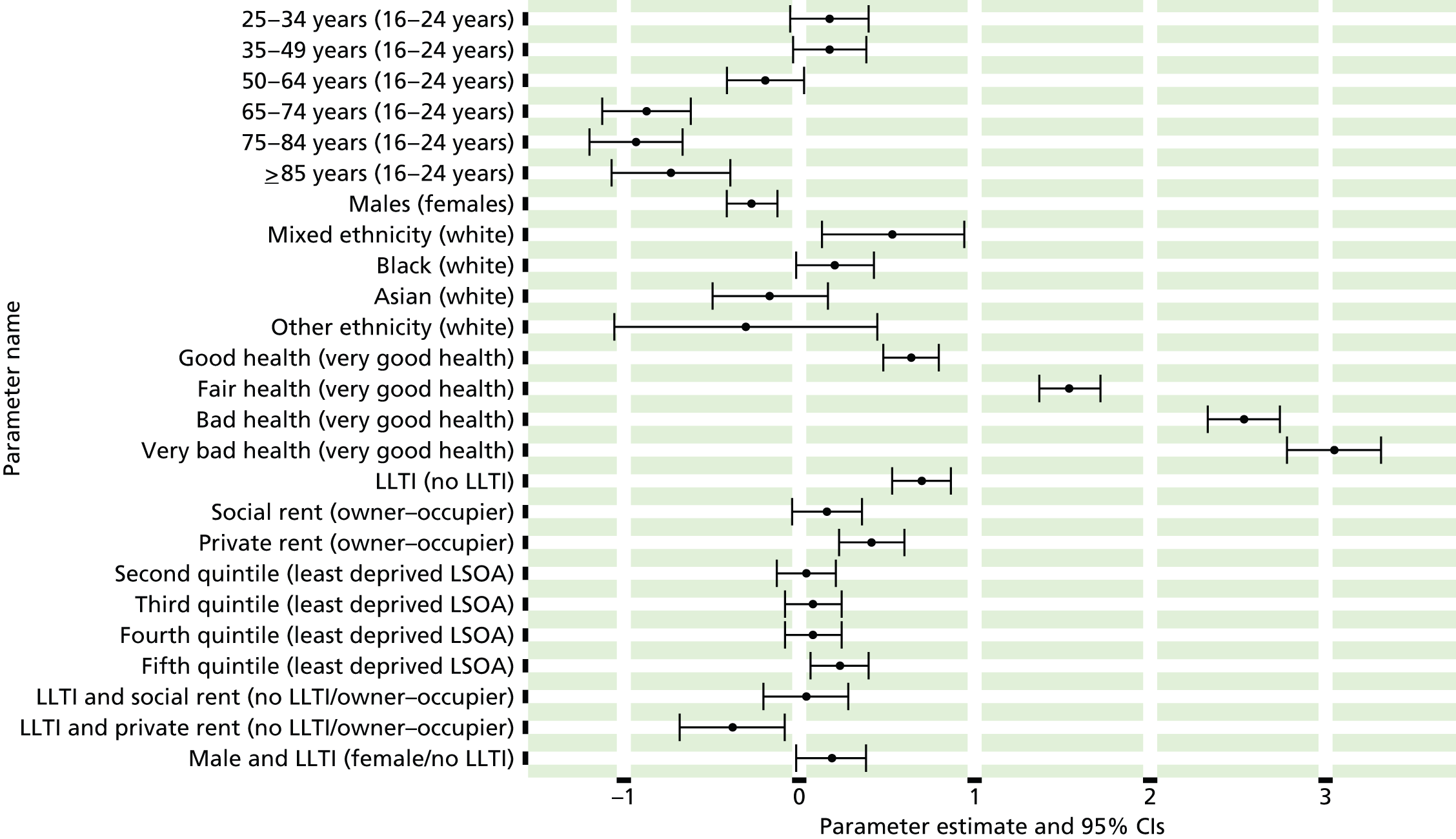
FIGURE 119.
‘Probable’ psychiatric morbidity (HSfE GHQ12 score of ≥ 6): individual estimates and their 95% CIs. (a) MSOAs; (b) LAs; (c) CCGs; and (d) regions (GORs).
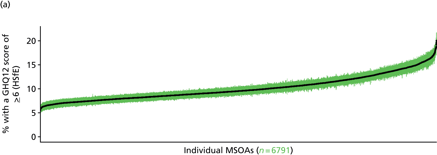
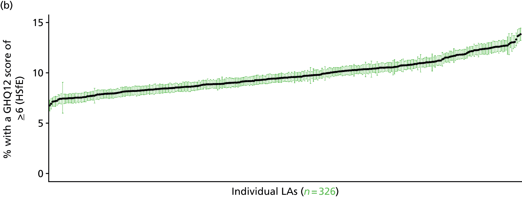
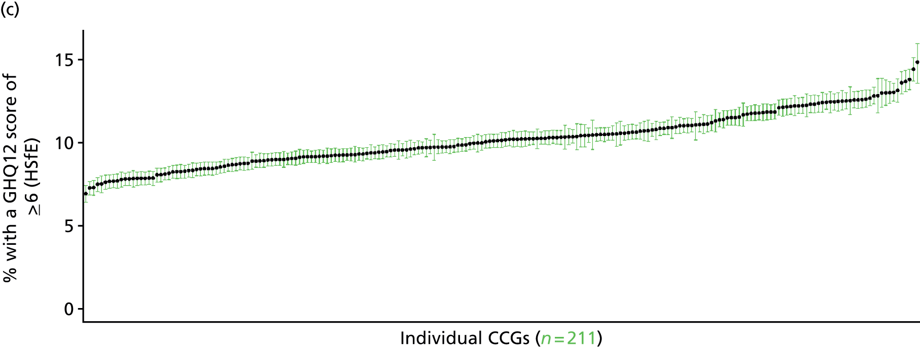
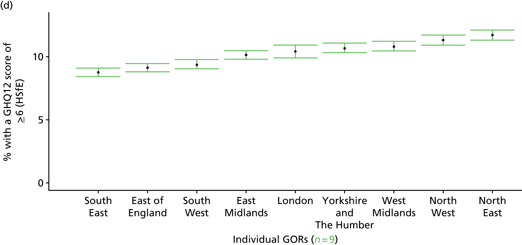
Psychiatric morbidity (12-item General Health Questionnaire score of ≥ 8) (Health Survey for England, 2006 and 2008–10)
FIGURE 120.
Psychiatric morbidity (HSfE GHQ12 score of ≥ 8): LSOA-level map. Contains Ordnance Survey data © Crown copyright and database right 2012.
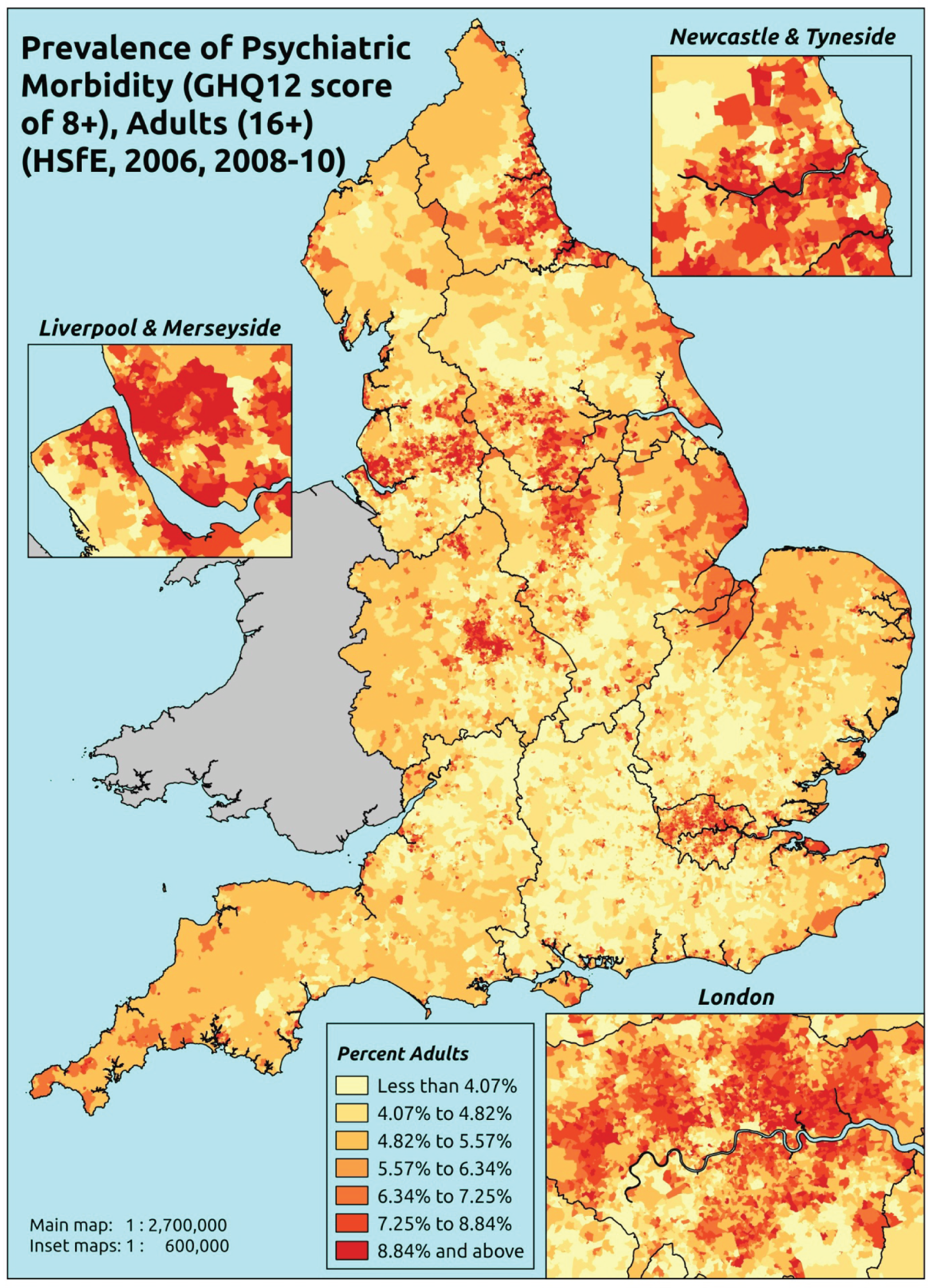
Response variable definition, provenance and prediction
Based on the GHQ12 incorporated within the HSfE in 2006 and 2008–10, here we capture whether or not people score ≥ 8 using the standard 0–12 ‘caseness’ scoring approach. The GHQ12 is a screening device for identifying minor psychiatric disorders in the general population. It assesses the respondent’s current state and asks if that differs from their usual state. It is sensitive to short-term psychiatric disorders but not long-standing attributes of the respondent. In the literature, a score of ≥ 4 is usually taken as being indicative of ‘possible psychiatric morbidity’, but occasionally ≥ 6 or ≥ 8 thresholds are used. For convenience (and without clinical justification) we describe a score of ≥ 8 as being indicative of ‘psychiatric morbidity’ – to distinguish it from the standard ≥ 4 threshold (‘possible psychiatric morbidity’) and the ≥ 6 threshold (‘probable psychiatric morbidity’). This is not independent of sociodemographic or geographic variations in access to, or uptake of, care, as individuals may score < 8 because they are currently being treated for a mental health issue. (See below for an alternative marker below which includes people currently being treated with medication for anxiety/depression.)
The HSfE at this time includes multiple household respondents of all ages. The analytical data set is drawn from a subset of respondents aged ≥ 16 years for whom data are available across all model response and predictor variables, namely whether or not they completed the GHQ12 questionnaire, along with information on age band, sex, ethnicity, general health status, LLTI, tenure and the IMD quintile of the LSOA of residence (n = 38,935). A single randomly selected adult is then drawn from each household, resulting in an analytical data set of 23,390 adults aged ≥ 16 years.
| Age band (years) | Females | Age band (years) | Males | ||||
|---|---|---|---|---|---|---|---|
| Does not have condition | Has condition | % | Does not have condition | Has condition | % | ||
| 16–24 | 979 | 49 | 4.8 | 16–24 | 698 | 14 | 2.0 |
| 25–34 | 1865 | 105 | 5.3 | 25–34 | 1198 | 55 | 4.4 |
| 35–49 | 3278 | 252 | 7.1 | 35–49 | 2325 | 164 | 6.6 |
| 50–64 | 2875 | 218 | 7.0 | 50–64 | 2311 | 174 | 7.0 |
| 65–74 | 1602 | 70 | 4.2 | 65–74 | 1323 | 54 | 3.9 |
| 75–84 | 1212 | 67 | 5.2 | 75–84 | 780 | 43 | 5.2 |
| ≥ 85 | 444 | 19 | 4.1 | ≥ 85 | 205 | 11 | 5.1 |
| Females | 12,255 | 780 | 6.0 | Males | 8840 | 515 | 5.5 |
| Total (males and females) | 21,095 | 1295 | 5.8 | ||||
Model parameters are applied to microsimulated LSOA-level census data to produce estimates of the number (and proportion) of people with psychiatric morbidity (i.e. who would score ≥ 8 on the GHQ12) in each age–sex cohort (and overall) in each of the 32,844 English LSOAs. As discussed in the report, bootstrapping is used to derive 95% CIs for the estimates. These LSOA-level prevalence rate estimates (and 95% CIs) are aggregated into a number of higher geographies, namely MSOAs, LAs, CCGs and regions (GORs). Proportionate attribution is used to restructure the prevalence rate estimates to align with 2001 MSOAs, as well as GP practice populations as defined by the 2011 NHS ADS.
Table 143 summarises how expected prevalence rates vary by age, sex and local deprivation (as measured by the 2010 IMD). There are 6569 LSOAs (with 9,226,227 adults) classified as being in the least deprived quintile; 6568 LSOAs (9,525,344 adults) in the second least deprived quintile; 6568 LSOAs (9,658,444 adults) in the third least deprived quintile; 6568 LSOAs (9,650,576 adults) in the fourth least deprived quintile; and 6568 LSOAs (9,535,167 adults) in the most deprived quintile. Note that, as a general rule, variations in prevalence rates reflect variations in the socioeconomic composition of populations in the different types of LSOA rather than variations in deprivation per se.
| Cohort | Least deprived quintile LSOAs | Second least deprived quintile LSOAs | Third least deprived quintile LSOAs | Fourth least deprived quintile LSOAs | Most deprived quintile LSOAs | All England |
|---|---|---|---|---|---|---|
| Female 16–24 | 2.2 (1.7 to 2.8) | 2.6 (2.0 to 3.2) | 3.0 (2.4 to 3.7) | 3.2 (2.6 to 3.8) | 4.0 (3.1 to 4.7) | 3.1 (2.5 to 3.7) |
| Female 25–34 | 3.0 (2.5 to 3.6) | 3.5 (3.1 to 4.4) | 4.2 (3.6 to 5.0) | 4.7 (4.0 to 5.5) | 6.1 (5.3 to 7.1) | 4.5 (4.0 to 5.2) |
| Female 35–49 | 4.6 (4.1 to 5.4) | 6.0 (5.3 to 6.7) | 7.5 (6.7 to 8.6) | 9.1 (7.9 to 10.1) | 12.6 (11.3 to 13.7) | 7.9 (7.3 to 8.6) |
| Female 50–64 | 4.8 (4.1 to 5.6) | 6.3(5.6 to 7.2) | 8.1 (7.3 to 9.3) | 10.3 (9.1 to 11.5) | 14.9 (13.2 to 16.3) | 8.6 (7.8 to 9.4) |
| Female F65–74 | 3.3 (2.7 to 4.0) | 4.3 (3.6 to 5.2) | 5.4 (4.6 to 6.5) | 6.7 (5.4 to 8.1) | 9.4 (7.9 to 11.0) | 5.6 (4.7 to 6.4) |
| Female ≥ 75 | 5.6 (4.7 to 6.6) | 6.9 (5.8 to 8.1) | 8.0 (6.8 to 9.6) | 9.1 (7.5 to 10.5) | 11.4 (9.6 to 13.3) | 8.0 (6.9 to 9.2) |
| Females | 4.2 (3.6 to 5.0) | 5.3 (4.6 to 6.2) | 6.4 (5.6 to 7.5) | 7.5 (6.4 to 8.5) | 10.0 (8.7 to 11.2) | 6.7 (6.0 to 7.5) |
| Male 16–24 | 1.8 (1.4 to 2.3) | 2.2 (1.6 to 2.7) | 2.5 (2.1 to 3.3) | 2.8 (2.3 to 3.4) | 3.6 (2.8 to 4.2) | 2.7 (2.2 to 3.2) |
| Male 25–34 | 2.6 (2.2 to 3.1) | 3.1 (2.6 to 3.8) | 3.6 (3.2 to 4.4) | 4.0 (3.5 to 4.8) | 5.5 (4.7 to 6.4) | 4.0 (3.5 to 4.6) |
| Male 35–49 | 3.9 (3.4 to 4.5) | 5.0 (4.3 to 5.8) | 6.4 (5.7 to 7.5) | 7.9 (6.7 to 8.8) | 11.3 (10.1 to 12.5) | 6.9 (6.3 to 7.6) |
| Male 50–64 | 4.2 (3.7 to 4.9) | 5.7 (5.0 to 6.5) | 7.4 (6.6 to 8.5) | 9.4 (8.2 to 10.6) | 13.6 (12.2 to 15.0) | 7.8 (7.2 to 8.6) |
| Male 65–74 | 3.0 (2.4 to 3.6) | 3.9 (3.3 to 4.9) | 5.0 (4.1 to 6.0) | 6.1 (5.0 to 7.4) | 8.7 (7.2 to 10.1) | 5.1 (4.3 to 5.9) |
| Male ≥ 75 | 4.8 (4.0 to 5.7) | 5.9 (5.0 to 7.1) | 7.0 (5.9 to 8.4) | 7.9 (6.6 to 9.4) | 10.2 (8.6 to 12.0) | 6.9 (6.0 to 8.0) |
| Males | 3.6 (3.0 to 4.2) | 4.5 (3.9 to 5.4) | 5.6 (4.9 to 6.6) | 6.5 (5.6 to 7.5) | 9.0 (7.9 to 10.1) | 5.9 (5.3 to 6.6) |
| All | 3.9 (3.4 to 4.4) | 4.9 (4.4 to 5.5) | 6.0 (5.5 to 6.7) | 7.0 (6.3 to 7.7) | 9.5 (8.8 to 10.2) | 6.3 (6.0 to 6.6) |
| Factor (reference group) | Model coefficients | 95% CI | ||
|---|---|---|---|---|
| Estimate | SE | 2.5% CI | 97.50% | |
| (Intercept) | –4.68258 | 0.18342 | –5.04209 | –4.32307 |
| Age (16–24 years) | ||||
| 25–34 years | 0.21527 | 0.15801 | –0.09443 | 0.52496 |
| 35–49 years | 0.45692 | 0.14593 | 0.17089 | 0.74295 |
| 50–64 years | 0.02431 | 0.15113 | –0.27190 | 0.32052 |
| 65–74 years | –0.76521 | 0.17156 | –1.10147 | –0.42895 |
| 75–84 years | –0.68071 | 0.17569 | –1.02507 | –0.33636 |
| ≥ 85 years | –0.91962 | 0.24050 | –1.39100 | –0.44824 |
| Sex (females) | ||||
| Males | –0.11694 | 0.06318 | –0.24077 | 0.00688 |
| Ethnicity (white) | ||||
| Mixed | 0.24025 | 0.28141 | –0.31132 | 0.79182 |
| Black | 0.36136 | 0.13383 | 0.09906 | 0.62365 |
| Asian | –0.10964 | 0.20667 | –0.51472 | 0.29545 |
| Other | –0.00655 | 0.44022 | –0.86939 | 0.85629 |
| General health status (very good health) | ||||
| Good health | 0.82891 | 0.11949 | 0.59471 | 1.06311 |
| Fair health | 1.77662 | 0.12557 | 1.53050 | 2.02274 |
| Bad health | 2.84287 | 0.14081 | 2.56688 | 3.11885 |
| Very bad health | 3.34685 | 0.16826 | 3.01706 | 3.67664 |
| LLTI (no LTTI) | ||||
| LLTI | 0.77360 | 0.07991 | 0.61698 | 0.93022 |
| Tenure (owner–occupier) | ||||
| Social rent | 0.22477 | 0.07876 | 0.07040 | 0.37913 |
| Private rent or other tenure | 0.37511 | 0.09576 | 0.18742 | 0.56280 |
| LSOA deprivation quintile (least deprived quintile) | ||||
| Second LSOA deprivation quintile | 0.11868 | 0.11163 | –0.10011 | 0.33746 |
| Third LSOA deprivation quintile | 0.19225 | 0.10839 | –0.02020 | 0.40470 |
| Fourth LSOA deprivation quintile | 0.18515 | 0.10758 | –0.02571 | 0.39601 |
| Fifth LSOA deprivation quintile ( = most deprived) | 0.28001 | 0.10922 | 0.06594 | 0.49408 |
| No interaction effects | ||||
FIGURE 121.
Parameter plots: psychiatric morbidity (HSfE GHQ12 score of ≥ 8).
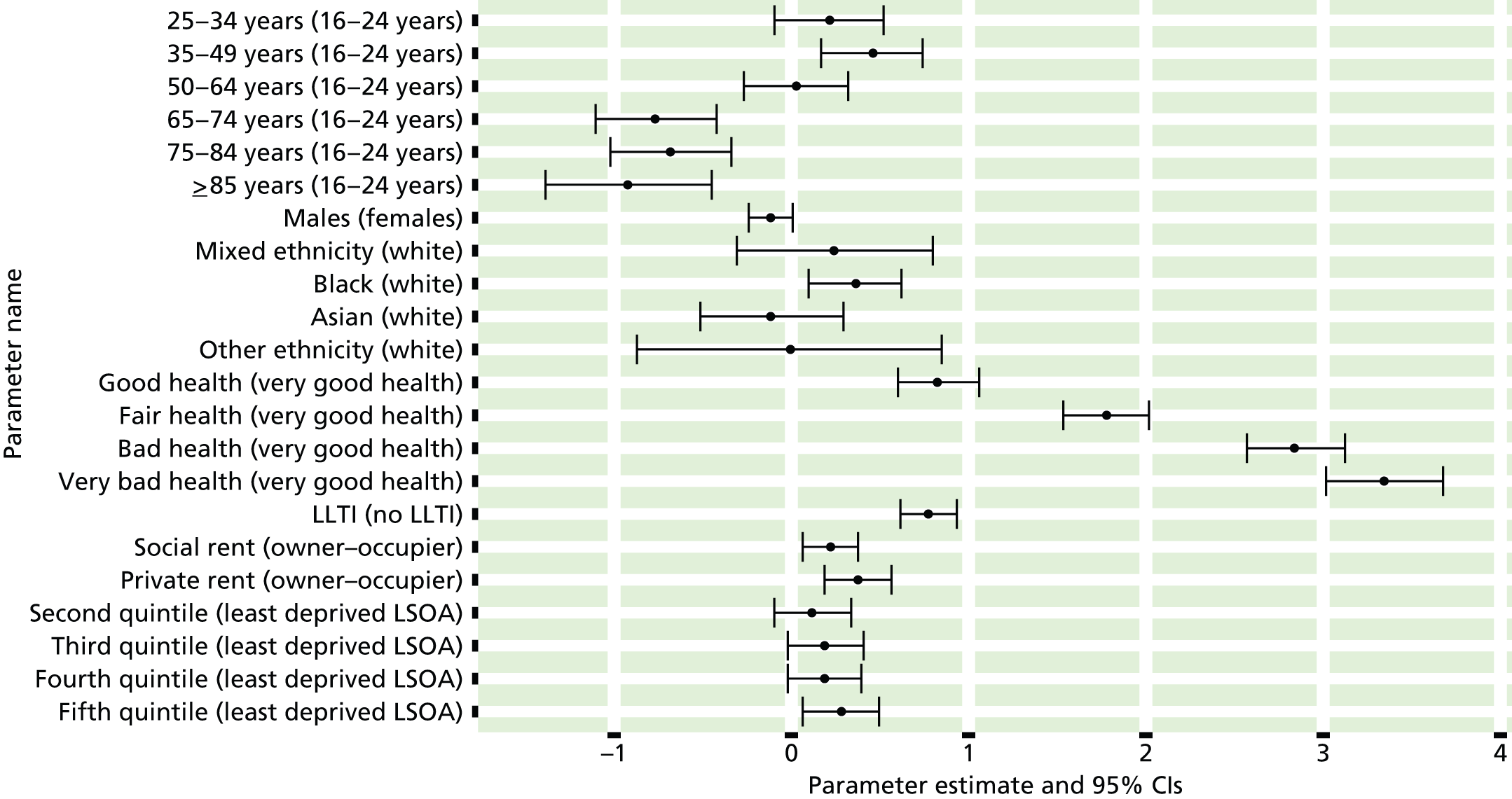
FIGURE 122.
Psychiatric morbidity (HSfE GHQ12 score of ≥ 8): individual estimates and their 95% CIs. (a) MSOAs; (b) LAs; (c) CCGs; and (d) regions (GORs).


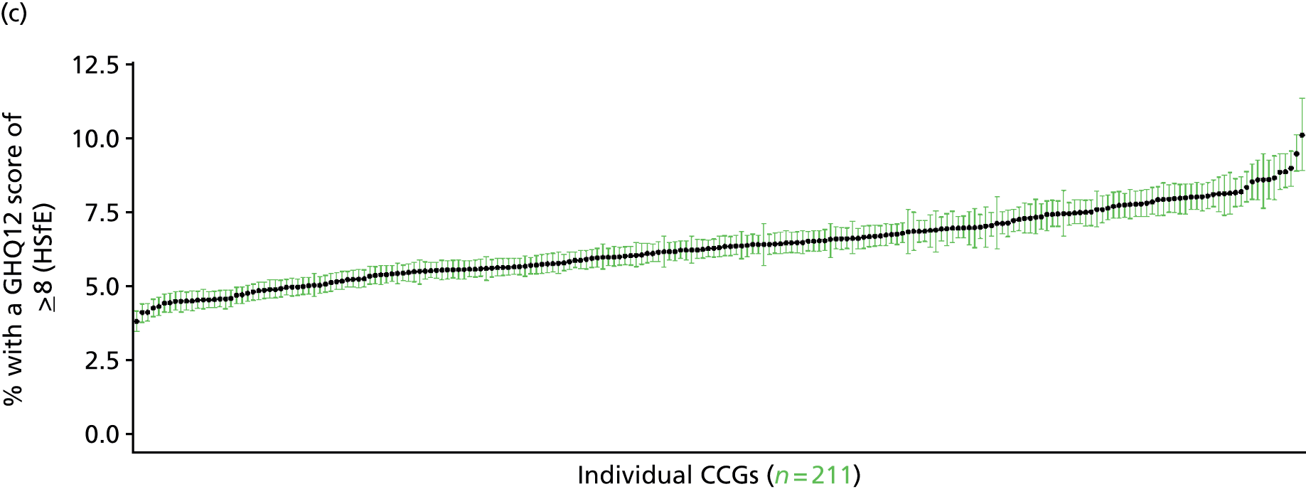
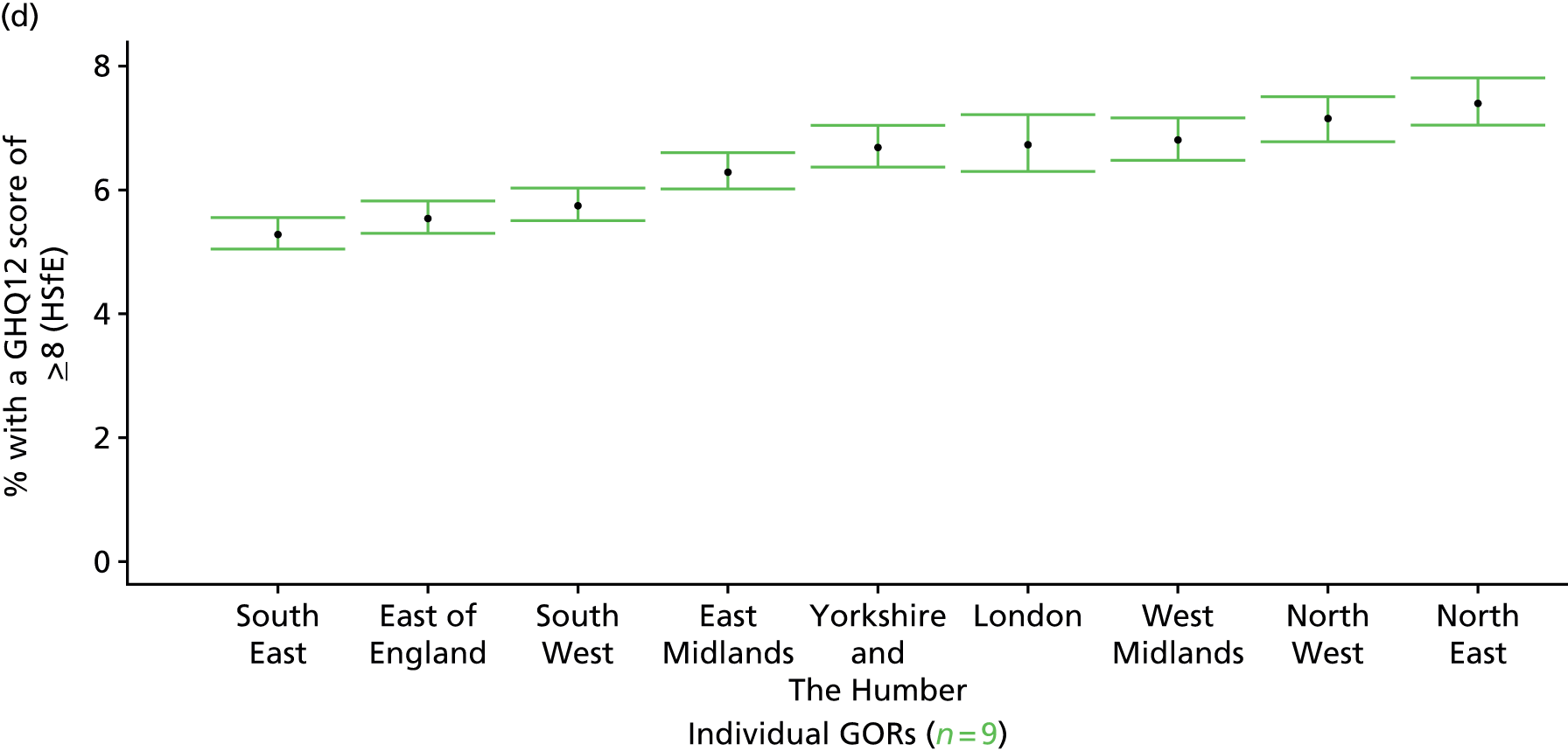
‘Possible’ psychiatric morbidity (12-item General Health Questionnaire score of ≥ 4) or currently prescribed depression/anxiety drugs (Health Survey for England, 2006 and 2008–10)
FIGURE 123.
‘Possible’ psychiatric morbidity (GHQ12 score of ≥ 4) or depression/anxiety drugs: LSOA-level map. Contains Ordnance Survey data © Crown copyright and database right 2012.
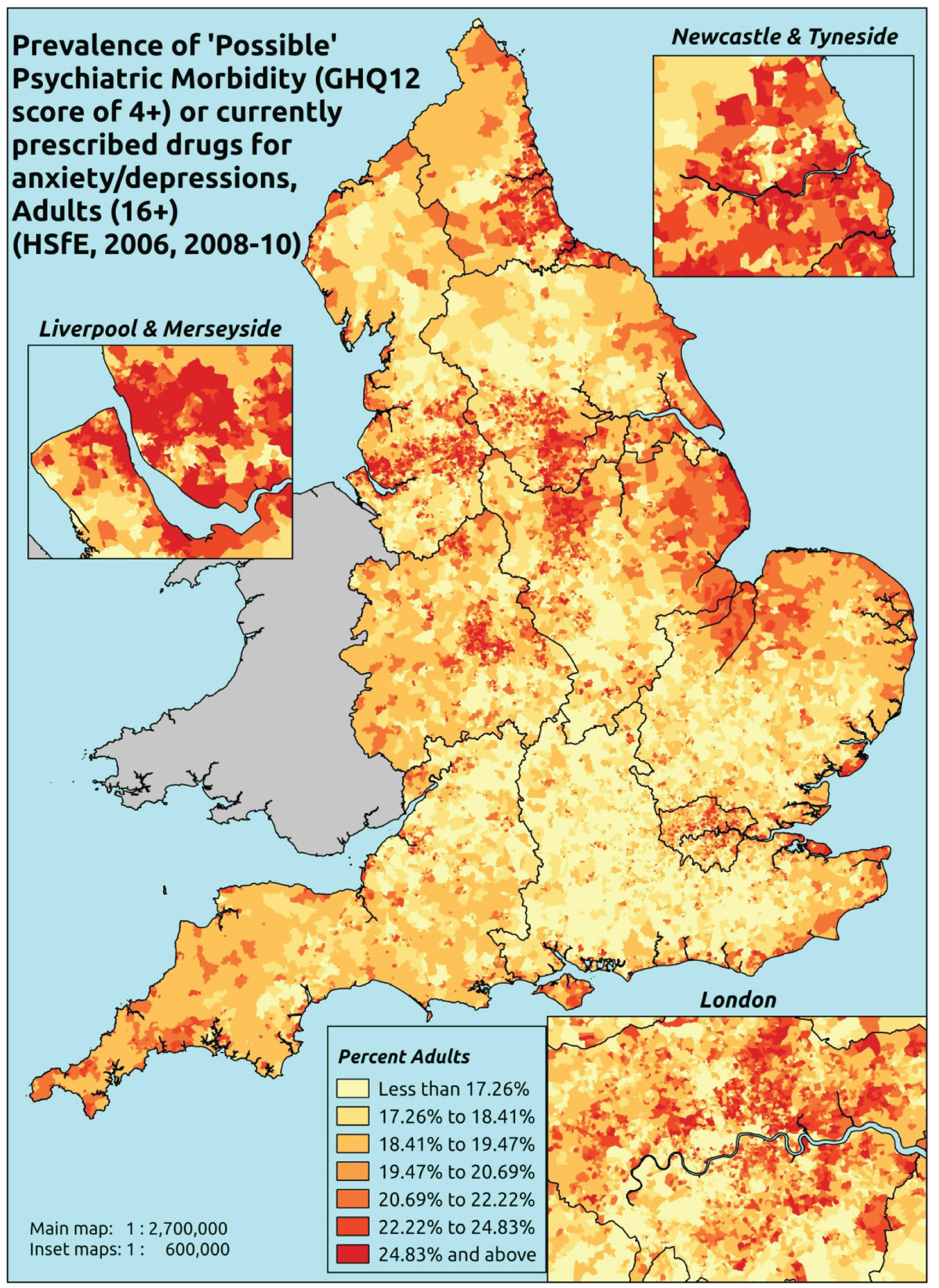
Response variable definition, provenance and prediction
Derived from the HSfE GHQ12 questionnaire score and questions about what medicines the respondent is currently being prescribed, this marker captures respondents with a GHQ12 score of ≥ 4 using the standard 0–12 ‘caseness’ scoring approach and/or who are currently being prescribed drugs for depression and/or anxiety (BNF 4.1.1–4.1.3 or 4.3.1–4.3.4487). In the literature, a score of ≥ 4 is usually taken as being indicative of ‘possible psychiatric morbidity’. We have no information regarding other forms of treatment for mental health issues. This recognises the fact that individuals may return a GHQ12 score of < 4 because they are being receiving medication for anxiety/depression and thus aims to capture underlying levels of ‘possible psychiatric morbidity’. This marker is affected by the fact that (a) other types of medication, and other forms of treatment, are not captured, and (b) any sociodemographic and/or geographic variations in access to, or uptake of, prescribing will affect rates of prescribing and thus this statistic.
The HSfE at this time includes multiple household respondents of all ages. The analytical data set is drawn from a subset of respondents aged ≥ 16 years for whom data are available across all model response and predictor variables, namely whether or not they completed the GHQ12 questionnaire, whether or not they completed question on medication currently being prescribed, along with information on age band, sex, ethnicity, general health status, LLTI, tenure and the IMD quintile of the LSOA of residence (n = 28,766). A single randomly selected adult is then drawn from each household, resulting in an analytical data set of 17,172 adults aged ≥ 16 years.
| Age band (years) | Females | Age band (years) | Males | ||||
|---|---|---|---|---|---|---|---|
| Does not have condition | Has condition | % | Does not have condition | Has condition | % | ||
| 16–24 | 577 | 143 | 19.9 | 16–24 | 442 | 45 | 9.2 |
| 25–34 | 1143 | 294 | 20.5 | 25–34 | 775 | 135 | 14.8 |
| 35–49 | 2137 | 631 | 22.8 | 35–49 | 1569 | 308 | 16.4 |
| 50–64 | 1925 | 623 | 24.5 | 50–64 | 1588 | 374 | 19.1 |
| 65–74 | 1017 | 307 | 23.2 | 65–74 | 908 | 153 | 14.4 |
| 75–84 | 712 | 225 | 24.0 | 75–84 | 558 | 114 | 17.0 |
| ≥ 85 | 219 | 82 | 27.2 | ≥ 85 | 125 | 43 | 25.6 |
| Females | 7730 | 2305 | 23.0 | Males | 5965 | 1172 | 16.4 |
| Total (males and females) | 13,695 | 3477 | 20.2 | ||||
Model parameters are applied to microsimulated LSOA-level census data to produce estimates of the number (and proportion) of people with treated or untreated ‘possible psychiatric morbidity (i.e. who would score ≥ 4 on the GHQ12 or be currently prescribed drugs for depression and/or anxiety) in each age–sex cohort (and overall) in each of the 32,844 English LSOAs. As discussed in the report, bootstrapping is used to derive 95% CIs for the estimates. These LSOA-level prevalence rate estimates (and 95% CIs) are aggregated into a number of higher geographies, namely MSOAs, LAs, CCGs and regions (GORs). Proportionate attribution is used to restructure the prevalence rate estimates to align with 2001 MSOAs, as well as GP practice populations as defined by the 2011 NHS ADS.
Table 146 summarises how expected prevalence rates vary by age, sex and local deprivation (as measured by the 2010 IMD). There are 6569 LSOAs (with 9,226,227 adults) classified as being in the least deprived quintile; 6568 LSOAs (9,525,344 adults) in the second least deprived quintile; 6568 LSOAs (9,658,444 adults) in the third least deprived quintile; 6568 LSOAs (9,650,576 adults) in the fourth least deprived quintile; and 6568 LSOAs (9,535,167 adults) in the most deprived quintile. Note that, as a general rule, variations in prevalence rates reflect variations in the socioeconomic composition of populations in the different types of LSOA rather than variations in deprivation per se.
| Cohort | Least deprived quintile LSOAs | Second least deprived quintile LSOAs | Third least deprived quintile LSOAs | Fourth least deprived quintile LSOAs | Most deprived quintile LSOAs | All England |
|---|---|---|---|---|---|---|
| Female 16–24 | 14.4 (12.1 to 16.0) | 13.7 (11.7 to 15.6) | 15.0 (13.0 to 16.8) | 14.7 (12.8 to 16.1) | 16.9 (15.0 to 18.6) | 15.1 (13.4 to 16.5) |
| Female 25–34 | 15.4 (14.1 to 17.3) | 15.2 (13.9 to 16.8) | 17.0 (15.7 to 18.6) | 17.4 (16.0 to 19.0) | 20.6 (19.3 to 22.6) | 17.5 (16.4 to 18.9) |
| Female 35–49 | 19.5 (18.1 to 20.9) | 19.9 (18.3 to 21.1) | 23.1 (21.4 to 24.5) | 24.9 (23.1 to 26.0) | 30.7 (29.0 to 32.4) | 23.6 (22.2 to 24.6) |
| Female 50–64 | 22.8 (21.4 to 24.3) | 23.6 (22.2 to 25.4) | 27.4 (26.0 to 29.3) | 30.2 (28.7 to 32.0) | 38.1 (36.4 to 40.2) | 27.9 (26.9 to 29.1) |
| Female 65–74 | 22.5 (21.0 to 24.3) | 23.2 (21.6 to 25.3) | 26.6 (25.0 to 28.8) | 28.9 (26.8 to 31.3) | 35.5 (33.5 to 38.5) | 26.8 (25.5 to 28.7) |
| Female ≥ 75 | 32.1 (30.1 to 34.8) | 31.8 (29.4 to 34.1) | 34.3 (31.8 to 36.6) | 34.4 (31.4 to 36.9) | 37.7 (34.8 to 40.4) | 33.9 (31.4 to 36.0) |
| Females | 21.5 (19.9 to 23.2) | 21.6 (20.0 to 23.4) | 24.1 (22.4 to 26.0) | 24.8 (22.9 to 26.5) | 29.2 (27.4 to 31.2) | 24.3 (22.8 to 25.7) |
| Male 16–24 | 9.4 (7.5 to 10.5) | 9.1 (7.6 to 10.4) | 10.3 (8.6 to 11.4) | 10.4 (8.8 to 11.4) | 12.8 (11.0 to 14.2) | 10.6 (9.1 to 11.6) |
| Male 25–34 | 10.3 (9.2 to 11.5) | 10.2 (9.1 to 11.5) | 11.7 (10.5 to 12.9) | 12.2 (10.9 to 13.4) | 15.6 (14.0 to 17.2) | 12.4 (11.2 to 13.5) |
| Male 35–49 | 12.4 (11.2 to 13.3) | 12.9 (11.8 to 13.8) | 15.5 (14.2 to 16.6) | 17.3 (15.8 to 18.1) | 23.1 (21.4 to 24.8) | 16.3 (15.2 to 17.0) |
| Male 50–64 | 15.0 (13.7 to 16.0) | 16.0 (14.9 to 17.2) | 19.5 (18.2 to 20.7) | 22.4 (20.9 to 23.7) | 29.9 (28.2 to 32.1) | 20.1 (19.1 to 21.1) |
| Male 65–74 | 15.4 (14.0 to 16.9) | 16.1 (14.9 to 17.8) | 19.3 (17.8 to 20.9) | 21.5 (19.5 to 23.5) | 27.6 (25.3 to 30.2) | 19.4 (18.2 to 21.0) |
| Male ≥ 75 | 21.4 (19.4 to 23.4) | 21.2 (19.1 to 23.2) | 23.4 (21.3 to 25.7) | 23.8 (21.1 to 26.0) | 27.4 (24.6 to 30.0) | 23.1 (21.2 to 25.0) |
| Males | 13.9 (12.5 to 15.1) | 14.2 (12.9 to 15.5) | 16.4 (15.0 to 17.7) | 17.4 (15.8 to 18.6) | 22.0 (20.2 to 23.9) | 16.8 (15.6 to 17.9) |
| All | 17.8 (16.9 to 18.7) | 18.0 (17.1 to 19.2) | 20.4 (19.4 to 21.2) | 21.2 (20.0 to 22.0) | 25.7 (24.7 to 26.9) | 20.7 (20.1 to 21.1) |
| Factor (reference group) | Model coefficients | 95% CI | ||
|---|---|---|---|---|
| Estimate | SE | 2.5% CI | 97.50% | |
| (Intercept) | –2.32901 | 0.14924 | –2.62152 | –2.03649 |
| Age (16–24 years) | ||||
| 25–34 years | 0.04924 | 0.15971 | –0.26379 | 0.36228 |
| 35–49 years | 0.16438 | 0.14381 | –0.11749 | 0.44626 |
| 50–64 years | 0.03141 | 0.14562 | –0.25401 | 0.31682 |
| 65–74 years | –0.28554 | 0.16262 | –0.60427 | 0.03319 |
| 75–84 years | –0.00782 | 0.17474 | –0.35030 | 0.33466 |
| ≥ 85 years | 0.21762 | 0.25343 | –0.27910 | 0.71433 |
| Sex (females) | ||||
| Males | –0.47154 | 0.10822 | –0.68365 | –0.25943 |
| Ethnicity (white) | ||||
| Mixed | –0.11832 | 0.36308 | –0.82996 | 0.59331 |
| Black | –0.19977 | 0.16804 | –0.52912 | 0.12959 |
| Asian | –0.19427 | 0.25430 | –0.69271 | 0.30416 |
| Other | –0.72772 | 0.64304 | –1.98808 | 0.53264 |
| General health status (very good health) | ||||
| Good health | 0.68028 | 0.07233 | 0.53852 | 0.82204 |
| Fair health | 1.36094 | 0.08376 | 1.19678 | 1.52510 |
| Bad health | 2.35796 | 0.11790 | 2.12688 | 2.58904 |
| Very bad health | 2.64420 | 0.19926 | 2.25365 | 3.03476 |
| LLTI (no LTTI) | ||||
| LLTI | 1.45229 | 0.22704 | 1.00730 | 1.89729 |
| Tenure (owner–occupier) | ||||
| Social rent | 0.15835 | 0.21563 | –0.26429 | 0.58099 |
| Private rent or other tenure | –0.08508 | 0.21658 | –0.50957 | 0.33942 |
| LSOA deprivation quintile (least deprived quintile) | ||||
| Second LSOA deprivation quintile | –0.09381 | 0.06676 | –0.22466 | 0.03705 |
| Third LSOA deprivation quintile | –0.01193 | 0.06607 | –0.14142 | 0.11756 |
| Fourth LSOA deprivation quintile | –0.08157 | 0.06824 | –0.21531 | 0.05218 |
| Fifth LSOA deprivation quintile ( = most deprived) | 0.02021 | 0.07179 | –0.12049 | 0.16092 |
| Interaction effects | ||||
| 25–34 years and social rent | 0.20927 | 0.25620 | –0.29288 | 0.71142 |
| 35–49 years and social rent | 0.16585 | 0.23547 | –0.29567 | 0.62737 |
| 50–64 years and social rent | 0.03035 | 0.23741 | –0.43498 | 0.49567 |
| 65–74 years and social rent | –0.22324 | 0.25682 | –0.72661 | 0.28014 |
| 75–84 years and social rent | –0.56359 | 0.26348 | –1.08000 | –0.04718 |
| ≥ 85 years and social rent | –0.79115 | 0.33310 | –1.44403 | –0.13828 |
| 25–34 years and private rent or other tenure | 0.53966 | 0.24958 | 0.05048 | 1.02884 |
| 35–49 years and private rent or other tenure | 0.37052 | 0.24375 | –0.10722 | 0.84826 |
| 50–64 years and private rent or other tenure | 0.50474 | 0.26743 | –0.01942 | 1.02891 |
| 65–74 years and private rent or other tenure | 0.42258 | 0.34206 | –0.24786 | 1.09301 |
| 75–84 years and private rent or other tenure | –0.33595 | 0.38606 | –1.09263 | 0.42074 |
| ≥ 85 years and private rent or other tenure | –0.57861 | 0.65217 | –1.85686 | 0.69964 |
| 25–34 years and LLTI | –0.66694 | 0.26550 | –1.18731 | –0.14657 |
| 35–49 years and LLTI | –0.61505 | 0.24347 | –1.09225 | –0.13785 |
| 50–64 years and LLTI | –0.72764 | 0.24130 | –1.20058 | –0.25469 |
| 65–74 years and LLTI | –0.71202 | 0.25528 | –1.21236 | –0.21168 |
| 75–84 years and LLTI | –1.07710 | 0.26491 | –1.59633 | –0.55788 |
| ≥ 85 years and LLTI | –0.87799 | 0.33306 | –1.53080 | –0.22519 |
| Mixed and social rent | –0.73038 | 0.58068 | –1.86852 | 0.40776 |
| Black and social rent | –0.16382 | 0.29972 | –0.75128 | 0.42364 |
| Asian and social rent | –0.50525 | 0.36274 | –1.21623 | 0.20572 |
| Other and social rent | 0.91178 | 0.86800 | –0.78951 | 2.61306 |
| Mixed and private rent or other tenure | 0.23844 | 0.53594 | –0.81201 | 1.28888 |
| Black and private rent or other tenure | –0.47916 | 0.30583 | –1.07858 | 0.12025 |
| Asian and private rent or other tenure | 0.95375 | 0.36011 | 0.24794 | 1.65956 |
| Other and private rent or other tenure | 1.88543 | 0.84468 | 0.22986 | 3.54100 |
| Male and social rent | 0.26229 | 0.11392 | 0.03901 | 0.48557 |
| Male and private rent or other tenure | –0.02100 | 0.13666 | –0.28885 | 0.24685 |
| Male and mixed | 0.75805 | 0.46967 | –0.16250 | 1.67860 |
| Male and black | 0.64727 | 0.22129 | 0.21355 | 1.08099 |
| Male and Asian | –0.27560 | 0.32960 | –0.92161 | 0.37040 |
| Male and other | –0.62026 | 0.79087 | –2.17036 | 0.92984 |
| Male and good health | –0.26949 | 0.12695 | –0.51831 | –0.02066 |
| Male and fair health | –0.00352 | 0.13236 | –0.26294 | 0.25590 |
| Male and bad health | –0.20120 | 0.17105 | –0.53647 | 0.13407 |
| Male and very bad health | 0.04755 | 0.28662 | –0.51422 | 0.60933 |
FIGURE 124.
Parameter plots: ‘possible’ psychiatric morbidity (HSfE GHQ12 score of ≥ 4) or depression/anxiety drugs.
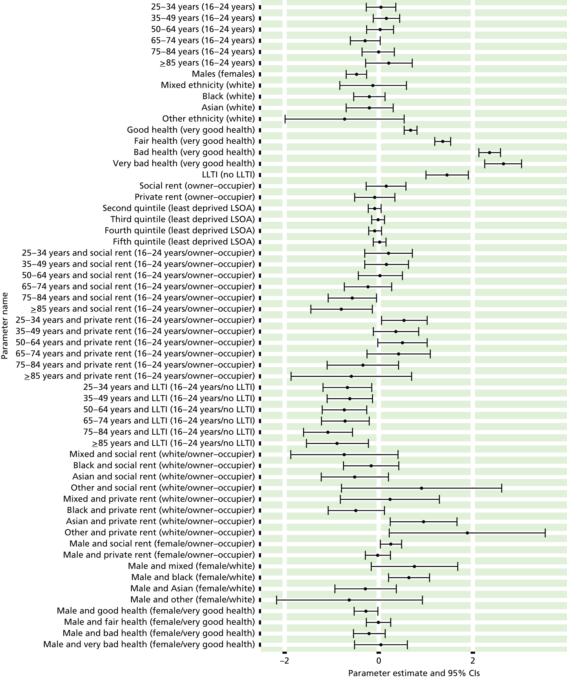
FIGURE 125.
‘Possible’ psychiatric morbidity (HSfE GHQ12 score of ≥ 4) or depression/anxiety drugs: individual estimates and their 95% CIs. (a) MSOAs; (b) LAs; (c) CCGs; and (d) regions (GORs).
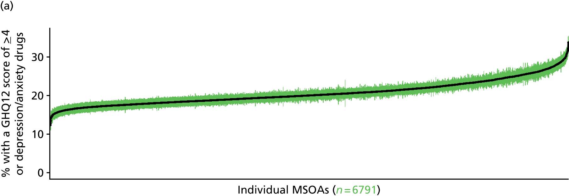
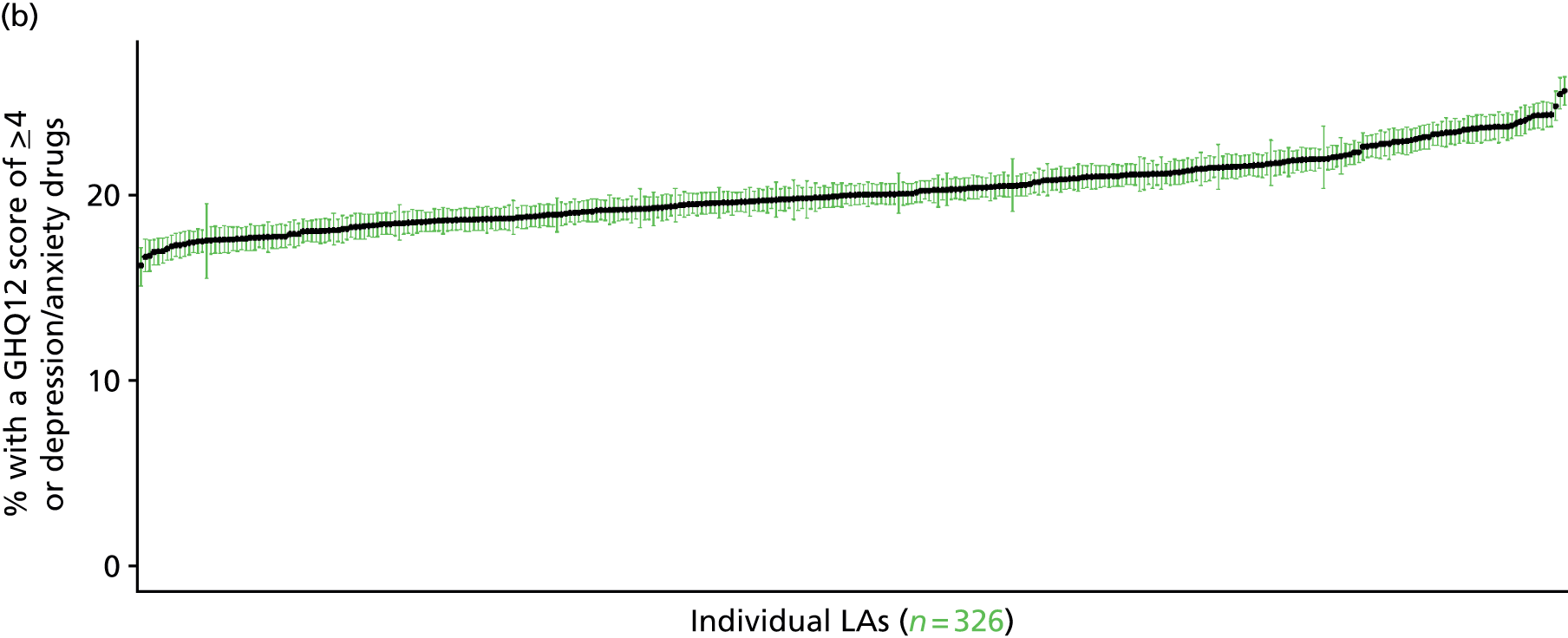

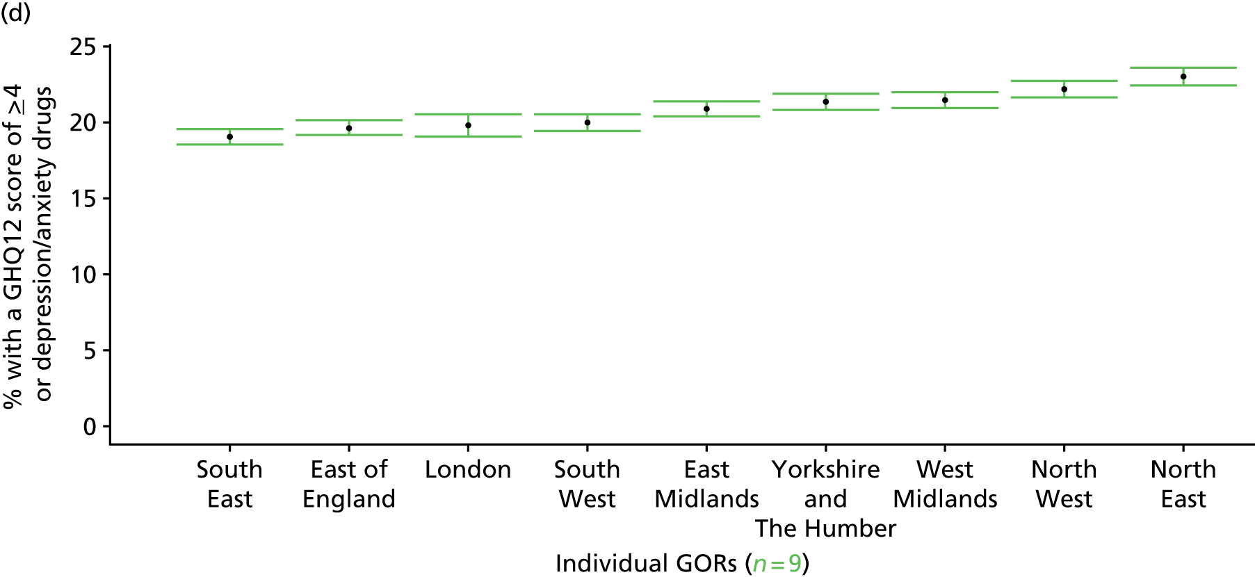
‘Probable’ psychiatric morbidity (12-item General Health Questionnaire score of ≥ 6) or currently prescribed depression/anxiety drugs (Health Survey for England, 2006 and 2008–10)
FIGURE 126.
‘Possible’ psychiatric morbidity (HSfE GHQ12 score of ≥ 6) or depression/anxiety drugs: LSOA-level map. Contains Ordnance Survey data © Crown copyright and database right 2012.
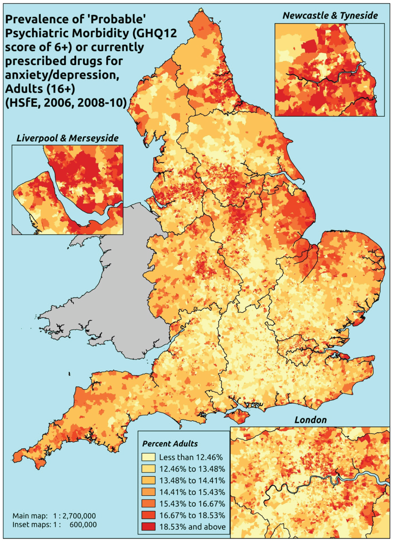
Response variable definition, provenance and prediction
Derived from the HSfE GHQ12 questionnaire score and questions about what medicines the respondent is currently being prescribed, this marker captures respondents with a GHQ12 score of ≥ 6 using the standard 0–12 ‘caseness’ scoring approach and/or who are currently being prescribed drugs for depression and/or anxiety (BNF 4.1.1–4.1.3 or 4.3.1–4.3.4487). In the literature, a score of ≥ 4 is usually taken as being indicative of ‘possible psychiatric morbidity’, but occasionally a ≥ 6 threshold is used. For convenience (and without clinical justification) we describe this as a marker of ‘probable psychiatric morbidity’ – to distinguish this marker from those using the standard ≥ 4 threshold (‘possible psychiatric morbidity’) and the higher ≥ 8 threshold (‘psychiatric morbidity’). We have no information regarding other forms of treatment for mental health issues. This marker recognises the fact that individuals may return a GHQ12 score of < 6 because they are being receiving medication for anxiety/depression and thus aims to capture underlying levels of ‘probable psychiatric morbidity’. This marker is affected by (a) the fact that other types of medication, and other forms of treatment, are not captured, and (b) any sociodemographic and/or geographic variations in access to, or uptake of, prescribing.
The HSfE at this time includes multiple household respondents of all ages. The analytical data set is drawn from a subset of respondents aged ≥ 16 years for whom data is available across all model response and predictor variables, namely whether or not they completed the GHQ12 questionnaire, whether or not they completed question on medication currently being prescribed, along with information on age band, sex, ethnicity, general health status, LLTI, tenure and the IMD quintile of the LSOA of residence (n = 28,766). A single randomly selected adult is then drawn from each household, resulting in an analytical data set of 17,172 adults aged ≥ 16 years.
| Age band (years) | Females | Age band (years) | Males | ||||
|---|---|---|---|---|---|---|---|
| Does not have condition | Has condition | % | Does not have condition | Has condition | % | ||
| 16–24 | 638 | 82 | 11.4 | 16–24 | 461 | 26 | 5.3 |
| 25–34 | 1224 | 213 | 14.8 | 25–34 | 822 | 88 | 9.7 |
| 35–49 | 2267 | 501 | 18.1 | 35–49 | 1660 | 217 | 11.6 |
| 50–64 | 2039 | 509 | 20.0 | 50–64 | 1670 | 292 | 14.9 |
| 65–74 | 1090 | 234 | 17.7 | 65–74 | 935 | 126 | 11.9 |
| 75–84 | 756 | 181 | 19.3 | 75–84 | 595 | 77 | 11.5 |
| ≥ 85 | 236 | 65 | 21.6 | ≥ 85 | 140 | 28 | 16.7 |
| Females | 8250 | 1785 | 17.8 | Males | 6283 | 854 | 12.0 |
| Total (males and females) | 14,533 | 2639 | 15.4 | ||||
Model parameters are applied to microsimulated LSOA-level census data to produce estimates of the number (and proportion) of people with treated or untreated ‘probable psychiatric morbidity (i.e. who would score ≥ 6 on the GHQ12 or be currently prescribed drugs for depression and/or anxiety) in each age–sex cohort (and overall) in each of the 32,844 English LSOAs. As discussed in the report, bootstrapping is used to derive 95% CIs for the estimates. These LSOA-level prevalence rate estimates (and 95% CIs) are aggregated into a number of higher geographies, namely MSOAs, LAs, CCGs and regions (GORs). Proportionate attribution is used to restructure the prevalence rate estimates to align with 2001 MSOAs, as well as GP practice populations as defined by the 2011 NHS ADS.
Table 149 summarises how expected prevalence rates vary by age, sex and local deprivation (as measured by the 2010 IMD). There are 6569 LSOAs (with 9,226,227 adults) classified as being in the least deprived quintile; 6568 LSOAs (9,525,344 adults) in the second least deprived quintile; 6568 LSOAs (9,658,444 adults) in the third least deprived quintile; 6568 LSOAs (9,650,576 adults) in the fourth least deprived quintile; and 6568 LSOAs (9,535,167 adults) in the most deprived quintile. Note that, as a general rule, variations in prevalence rates reflect variations in the socioeconomic composition of populations in the different types of LSOA rather than variations in deprivation per se.
| Cohort | Least deprived quintile LSOAs | Second least deprived quintile LSOAs | Third least deprived quintile LSOAs | Fourth least deprived quintile LSOAs | Most deprived quintile LSOAs | All England |
|---|---|---|---|---|---|---|
| Female 16–24 | 8.9 (6.9 to 10.4) | 8.7 (6.9 to 10.3) | 9.3 (7.3 to 10.9) | 8.7 (6.9 to 10.0) | 9.9 (8.0 to 10.9) | 9.2 (7.3 to 10.4) |
| Female 25–34 | 10.3 (9.1 to 11.5) | 10.5 (9.2 to 11.9) | 11.8 (10.6 to 13.0) | 11.9 (10.6 to 13.3) | 14.3 (12.6 to 15.5) | 12.0 (10.9 to 13.2) |
| Female 35–49 | 14.7 (13.4 to 15.9) | 15.7 (14.5 to 16.9) | 18.2 (16.9 to 19.6) | 19.3 (18.0 to 20.4) | 24.3 (22.3 to 25.6) | 18.4 (17.3 to 19.2) |
| Female 50–64 | 17.9 (16.7 to 19.3) | 19.4 (17.8 to 20.9) | 22.6 (21.0 to 24.2) | 24.7 (22.9 to 26.7) | 31.6 (29.6 to 33.6) | 22.8 (21.7 to 24.0) |
| Female 65–74 | 17.5 (16.1 to 19.2) | 18.6 (17.2 to 20.9) | 21.2 (19.6 to 23.7) | 22.6 (20.7 to 25.1) | 27.8 (25.1 to 30.9) | 21.1 (19.6 to 23.3) |
| Female ≥ 75 | 24.3 (21.8 to 26.6) | 24.7 (22.7 to 27.4) | 26.9 (24.4 to 29.6) | 26.4 (23.9 to 29.6) | 29.1 (25.7 to 32.4) | 26.1 (23.9 to 28.4) |
| Females | 16.1 (14.6 to 17.6) | 16.8 (15.3 to 18.5) | 18.7 (17.1 to 20.5) | 18.8 (17.1 to 20.6) | 22.3 (20.2 to 24.1) | 18.6 (17.2 to 19.9) |
| Male 16–24 | 5.1 (3.8 to 5.9) | 5.1 (3.9 to 6.0) | 5.6 (4.3 to 6.6) | 5.5 (4.3 to 6.3) | 6.6 (5.3 to 7.5) | 5.7 (4.5 to 6.5) |
| Male 25–34 | 6.1 (5.2 to 6.9) | 6.3 (5.5 to 7.1) | 7.3 (6.3 to 8.0) | 7.5 (6.6 to 8.4) | 9.8 (8.5 to 10.8) | 7.7 (6.8 to 8.4) |
| Male 35–49 | 8.5 (7.4 to 9.1) | 9.3 (8.3 to 10.0) | 11.3 (10.2 to 12.2) | 12.6 (11.4 to 13.3) | 17.1 (15.3 to 18.3) | 11.8 (10.9 to 12.3) |
| Male 50–64 | 11.1 (10.1 to 12.0) | 12.5 (11.4 to 13.6) | 15.4 (14.0 to 16.6) | 17.5 (16.1 to 19.0) | 23.7 (21.5 to 25.4) | 15.7 (14.5 to 16.7) |
| Male 65–74 | 11.4 (10.2 to 12.6) | 12.4 (11.2 to 13.9) | 14.7 (13.1 to 16.3) | 16.1 (14.1 to 17.7) | 20.4 (17.7 to 22.9) | 14.6 (13.1 to 16.0) |
| Male ≥ 75 | 15.6 (13.6 to 17.3) | 16.0 (13.9 to 18.1) | 17.7 (15.6 to 19.9) | 17.5 (15.4 to 19.8) | 20.1 (17.5 to 22.5) | 17.2 (15.1 to 19.0) |
| Males | 9.7 (8.5 to 10.6) | 10.3 (9.2 to 11.5) | 12.0 (10.6 to 13.1) | 12.4 (11.1 to 13.5) | 15.8 (14.0 to 17.2) | 12.0 (10.9 to 13.0) |
| All | 13.0 (12.2 to 13.6) | 13.7 (12.8 to 14.6) | 15.4 (14.4 to 16.3) | 15.7 (14.8 to 16.5) | 19.1 (17.7 to 20.0) | 15.4 (14.9 to 15.8) |
| Factor (reference group) | Model coefficients | 95% CI | ||
|---|---|---|---|---|
| Estimate | SE | 2.5% CI | 97.50% | |
| (Intercept) | –2.86204 | 0.17788 | –3.21068 | –2.51339 |
| Age (16–24 years) | ||||
| 25–34 years | 0.00094 | 0.19628 | –0.38378 | 0.38566 |
| 35–49 years | 0.29348 | 0.17498 | –0.04948 | 0.63644 |
| 50–64 years | 0.18754 | 0.17670 | –0.15880 | 0.53387 |
| 65–74 years | –0.04246 | 0.19359 | –0.42189 | 0.33697 |
| 75–84 years | 0.13642 | 0.20767 | –0.27061 | 0.54345 |
| ≥ 85 years | 0.47105 | 0.28579 | –0.08909 | 1.03120 |
| Sex (females) | ||||
| Males | –0.73582 | 0.07175 | –0.87646 | –0.59519 |
| Ethnicity (white) | ||||
| Mixed | –0.14256 | 0.40955 | –0.94527 | 0.66016 |
| Black | –0.29866 | 0.19293 | –0.67679 | 0.07948 |
| Asian | –0.63512 | 0.32241 | –1.26704 | –0.00319 |
| Other | –0.31598 | 0.65049 | –1.59094 | 0.95897 |
| General health status (very good health) | ||||
| Good health | 0.69911 | 0.07229 | 0.55742 | 0.8408 |
| Fair health | 1.48802 | 0.08125 | 1.32876 | 1.64728 |
| Bad health | 2.39995 | 0.10217 | 2.19970 | 2.60020 |
| Very bad health | 2.65092 | 0.14959 | 2.35773 | 2.94411 |
| LLTI (no LTTI) | ||||
| LLTI | 1.24982 | 0.25548 | 0.74908 | 1.75055 |
| Tenure (owner–occupier) | ||||
| Social rent | –0.00890 | 0.26104 | –0.52055 | 0.50274 |
| Private rent or other tenure | –0.45962 | 0.27826 | –1.00502 | 0.08578 |
| LSOA deprivation quintile (least deprived quintile) | ||||
| Second LSOA deprivation quintile | –0.04814 | 0.07478 | –0.19470 | 0.09843 |
| Third LSOA deprivation quintile | 0.01863 | 0.07400 | –0.12642 | 0.16367 |
| Fourth LSOA deprivation quintile | –0.08191 | 0.07649 | –0.23182 | 0.06801 |
| Fifth LSOA deprivation quintile ( = most deprived) | –0.00947 | 0.08021 | –0.16669 | 0.14774 |
| Interaction effects | ||||
| 25–34 years and LLTI | –0.44615 | 0.29456 | –1.02348 | 0.13119 |
| 35–49 years and LLTI | –0.45808 | 0.27083 | –0.98890 | 0.07274 |
| 50–64 years and LLTI | –0.54919 | 0.26908 | –1.07659 | –0.02180 |
| 65–74 years and LLTI | –0.72293 | 0.28436 | –1.28028 | –0.16559 |
| 75–84 years and LLTI | –1.06358 | 0.29561 | –1.64297 | –0.48419 |
| ≥ 85 years and LLTI | –1.07771 | 0.36612 | –1.79530 | –0.36012 |
| 25–34 years and social rent | 0.53575 | 0.30703 | –0.06604 | 1.13754 |
| 35–49 years and social rent | 0.42664 | 0.28148 | –0.12507 | 0.97834 |
| 50–64 years and social rent | 0.33200 | 0.28129 | –0.21934 | 0.88333 |
| 65–74 years and social rent | 0.07932 | 0.30143 | –0.51147 | 0.67012 |
| 75–84 years and social rent | –0.15384 | 0.30914 | –0.75977 | 0.45208 |
| ≥ 85 years and social rent | –0.42411 | 0.37953 | –1.16800 | 0.31977 |
| 25–34 years and private rent or other tenure | 1.10127 | 0.31784 | 0.47830 | 1.72424 |
| 35–49 years and private rent or other tenure | 0.75179 | 0.30851 | 0.14710 | 1.35647 |
| 50–64 years and private rent or other tenure | 0.79283 | 0.32917 | 0.14766 | 1.43800 |
| 65–74 years and private rent or other tenure | 0.70331 | 0.40304 | –0.08665 | 1.49327 |
| 75–84 years and private rent or other tenure | 0.50429 | 0.42625 | –0.33117 | 1.33975 |
| ≥ 85 years and private rent or other tenure | –0.12219 | 0.73102 | –1.55499 | 1.31062 |
| Male and mixed | 1.11218 | 0.50534 | 0.12171 | 2.10266 |
| Male and black | 0.75804 | 0.25173 | 0.26466 | 1.25142 |
| Male and Asian | –0.13211 | 0.41563 | –0.94674 | 0.68252 |
| Male and other | –0.58103 | 1.23779 | –3.00710 | 1.84504 |
| Male and LLTI | 0.22687 | 0.09893 | 0.03297 | 0.42078 |
| Mixed and social rent | –0.33906 | 0.60230 | –1.51956 | 0.84145 |
| Black and social rent | 0.13731 | 0.32131 | –0.49246 | 0.76707 |
| Asian and social rent | –0.47684 | 0.46055 | –1.37951 | 0.42583 |
| Other and social rent | 0.21347 | 0.95791 | –1.66404 | 2.09098 |
| Mixed and private rent or other tenure | –0.00332 | 0.60656 | –1.19218 | 1.18553 |
| Black and private rent or other tenure | –0.70847 | 0.37687 | –1.44713 | 0.03018 |
| Asian and private rent or other tenure | 1.05923 | 0.43807 | 0.20062 | 1.91785 |
| Other and private rent or other tenure | –0.99346 | 1.32161 | –3.58381 | 1.59690 |
FIGURE 127.
Parameter plots: ‘possible’ psychiatric morbidity (HSfE GHQ12 score of ≥ 6) or depression/anxiety drugs.
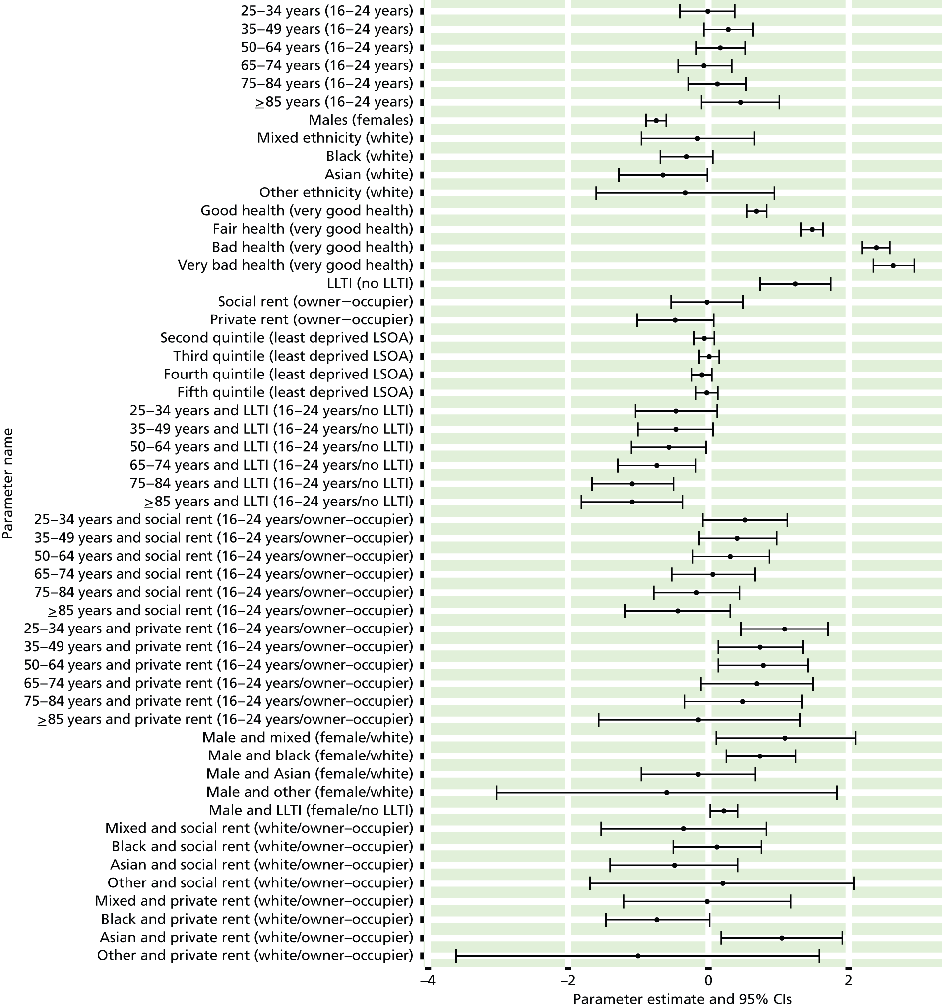
FIGURE 128.
‘Possible’ psychiatric morbidity (HSfE GHQ12 score of ≥ 6) or depression/anxiety drugs: individual estimates and their 95% CIs. (a) MSOAs; (b) LAs; (c) CCGs; and (d) regions (GORs).


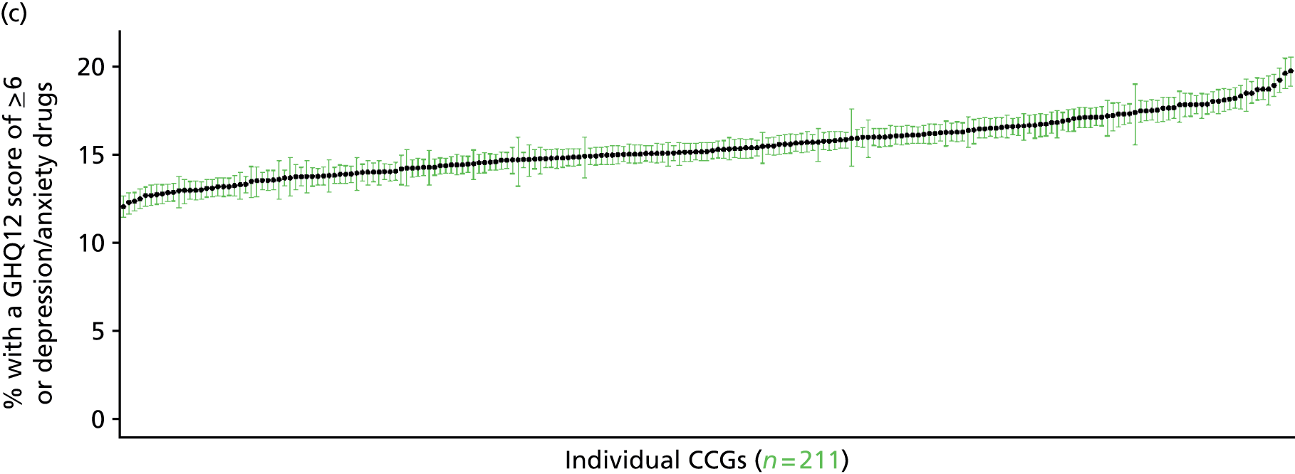
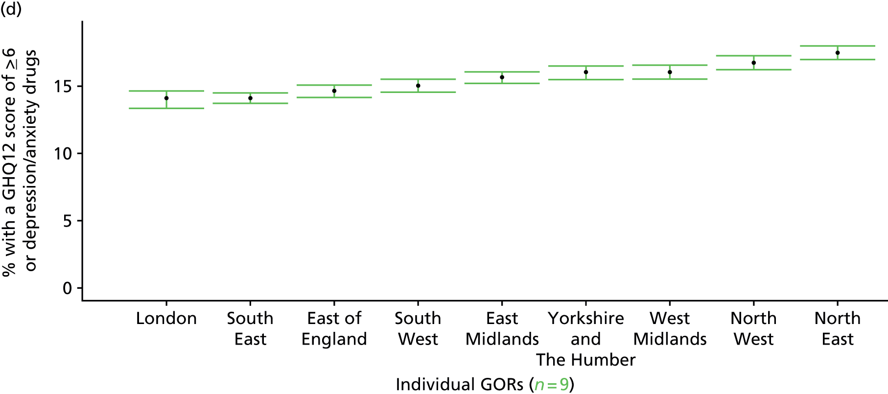
Psychiatric morbidity (12-item General Health Questionnaire score of ≥ 8) or currently prescribed depression/anxiety drugs (Health Survey for England, 2006 and 2008–10)
FIGURE 129.
Psychiatric morbidity (HSfE GHQ12 score of ≥ 8) or depression/anxiety drugs: LSOA-level map. Contains Ordnance Survey data © Crown copyright and database right 2012.
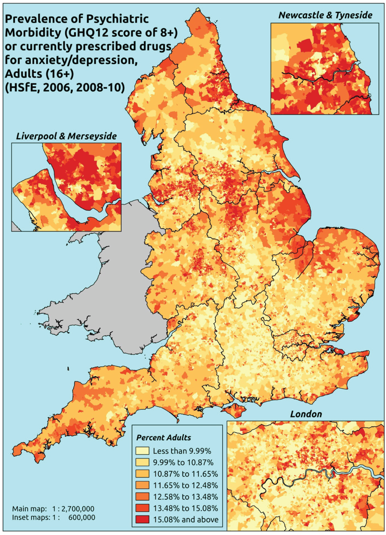
Response variable definition, provenance and prediction
Derived from the HSfE GHQ12 questionnaire score and questions about what medicines the respondent is currently being prescribed, this marker captures respondents with a GHQ12 score of ≥ 8 using the standard 0–12 ‘caseness’ scoring approach and/or who are currently being prescribed drugs for depression and/or anxiety (BNF 4.1.1–4.1.3 or 4.3.1–4.3.4487). In the literature, a score of ≥ 4 is usually taken as being indicative of ‘possible psychiatric morbidity’, but occasionally ≥ 6 or ≥ 8 thresholds are used. For convenience (and without clinical justification) we describe this as a marker of ‘psychiatric morbidity’ – to distinguish it from the standard ≥ 4 threshold (‘possible psychiatric morbidity’) and the ≥ 6 threshold (‘probable psychiatric morbidity’). We have no information regarding other forms of treatment for mental health issues. This marker recognises the fact that individuals may return a GHQ12 score of < 8 because they are receiving medication for anxiety/depression and thus aims to capture underlying levels of ‘probable psychiatric morbidity’. This marker is affected by (a) the fact that other types of medication, and other forms of treatment, are not captured, and (b) any sociodemographic and/or geographic variations in access to, or uptake of, prescribing.
The HSfE at this time includes multiple household respondents of all ages. The analytical data set is drawn from a subset of respondents aged ≥ 16 years for whom data are available across all model response and predictor variables, namely whether or not they completed the GHQ12 questionnaire and whether or not they completed question on medication currently being prescribed, along with information on age band, sex, ethnicity, general health status, LLTI, tenure and the IMD quintile of the LSOA of residence (n = 28,766). A single randomly selected adult is then drawn from each household, resulting in an analytical data set of 17,172 adults aged ≥ 16 years.
| Age band (years) | Females | Age band (years) | Males | ||||
|---|---|---|---|---|---|---|---|
| Does not have condition | Has condition | % | Does not have condition | Has condition | % | ||
| 16–24 | 669 | 51 | 7.1 | 16–24 | 474 | 13 | 2.7 |
| 25–34 | 1271 | 166 | 11.6 | 25–34 | 849 | 61 | 6.7 |
| 35–49 | 2345 | 423 | 15.3 | 35–49 | 1708 | 169 | 9.0 |
| 50–64 | 2119 | 429 | 16.8 | 50–64 | 1731 | 231 | 11.8 |
| 65–74 | 1119 | 205 | 15.5 | 65–74 | 958 | 103 | 9.7 |
| 75–84 | 774 | 163 | 17.4 | 75–84 | 608 | 64 | 9.5 |
| ≥ 85 | 247 | 54 | 17.9 | ≥ 85 | 147 | 21 | 12.5 |
| Females | 8544 | 1491 | 14.9 | Males | 6475 | 662 | 9.3 |
| Total (males and females) | 15,019 | 2153 | 12.5 | ||||
Model parameters are applied to microsimulated LSOA-level census data to produce estimates of the number (and proportion) of people with treated or untreated ‘psychiatric morbidity (i.e. who would score ≥ 8 on the GHQ12 or be currently prescribed drugs for depression and/or anxiety) in each age–sex cohort (and overall) in each of the 32,844 English LSOAs. As discussed in the report, bootstrapping is used to derive 95% CIs for the estimates. These LSOA-level prevalence rate estimates (and 95% CIs) are aggregated into a number of higher geographies, namely MSOAs, LAs, CCGs and regions (GORs). Proportionate attribution is used to restructure the prevalence rate estimates to align with 2001 MSOAs, as well as GP practice populations as defined by the 2011 NHS ADS.
Table 152 summarises how expected prevalence rates vary by age, sex and local deprivation (as measured by the 2010 IMD). There are 6569 LSOAs (with 9,226,227 adults) classified as being in the least deprived quintile; 6568 LSOAs (9,525,344 adults) in the second least deprived quintile; 6568 LSOAs (9,658,444 adults) in the third least deprived quintile; 6568 LSOAs (9,650,576 adults) in the fourth least deprived quintile; and 6568 LSOAs (9,535,167 adults) in the most deprived quintile. Note that, as a general rule, variations in prevalence rates reflect variations in the socioeconomic composition of populations in the different types of LSOA rather than variations in deprivation per se.
| Cohort | Least deprived quintile LSOAs | Second least deprived quintile LSOAs | Third least deprived quintile LSOAs | Fourth least deprived quintile LSOAs | Most deprived quintile LSOAs | All England |
|---|---|---|---|---|---|---|
| Female 16–24 | 4.9 (3.6 to 6.0) | 4.8 (3.5 to 6.0) | 5.3 (3.9 to 6.5) | 5.0 (3.9 to 6.1) | 6.1 (4.7 to 7.2) | 5.3 (4.0 to 6.4) |
| Female 25–34 | 7.9 (6.8 to 8.9) | 8.0 (6.9 to 9.1) | 8.9 (7.9 to 10.1) | 8.8 (7.9 to 10.1) | 11.0 (9.4 to 11.9) | 9.1 (8.2 to 10.1) |
| Female 35–49 | 12.4 (11.2 to 13.4) | 13.1 (12.2 to 14.4) | 15.3 (13.9 to 16.6) | 16.1 (14.9 to 17.4) | 20.8 (19.2 to 22.1) | 15.5 (14.6 to 16.4) |
| Female 50–64 | 15.2 (13.9 to 16.7) | 16.5 (15.3 to 18.1) | 19.3 (17.9 to 20.9) | 21.0 (19.5 to 22.6) | 27.6 (25.4 to 29.8) | 19.5 (18.4 to 20.7) |
| Female 65–74 | 15.4 (13.9 to 17.1) | 16.2 (14.6 to 18.2) | 18.5 (16.9 to 20.6) | 19.2 (17.3 to 21.4) | 24.1 (21.5 to 26.6) | 18.3 (16.8 to 19.9) |
| Female ≥ 75 | 21.7 (19.4 to 23.8) | 21.9 (19.7 to 24.7) | 23.7 (20.8 to 26.0) | 22.6 (19.8 to 25.5) | 25.1 (22.2 to 27.9) | 22.9 (20.6 to 25.1) |
| Females | 13.5 (12.1 to 14.9) | 14.1 (12.7 to 15.7) | 15.6 (14.0 to 17.2) | 15.3 (13.9 to 17.0) | 18.7 (16.8 to 20.3) | 15.4 (14.2 to 16.7) |
| Male 16–24 | 2.5 (1.8 to 3.2) | 2.6 (1.8 to 3.3) | 2.9 (2.2 to 3.6) | 2.9 (2.2 to 3.6) | 3.8 (2.9 to 4.6) | 3.0 (2.3 to 3.7) |
| Male 25–34 | 4.2 (3.6 to 4.9) | 4.4 (3.7 to 5.0) | 5.0 (4.3 to 5.7) | 5.1 (4.4 to 5.9) | 6.9 (5.8 to 7.7) | 5.3 (4.6 to 6.0) |
| Male 35–49 | 6.5 (5.6 to 7.2) | 7.1 (6.4 to 7.8) | 8.7 (7.9 to 9.5) | 9.6 (8.6 to 10.6) | 13.6 (12.4 to 14.6) | 9.1 (8.4 to 9.8) |
| Male 50–64 | 8.7 (7.8 to 9.6) | 9.9 (8.9 to 10.8) | 12.2 (11.1 to 13.3) | 13.8 (12.7 to 15.0) | 19.3 (17.7 to 20.9) | 12.5 (11.7 to 13.3) |
| Male 65–74 | 9.2 (8.1 to 10.3) | 10.0 (8.9 to 11.3) | 11.9 (10.6 to 13.2) | 12.6 (11.0 to 14.1) | 16.3 (14.1 to 18.3) | 11.7 (10.5 to 13.0) |
| Male ≥ 75 | 13.0 (11.3 to 14.2) | 13.1 (11.6 to 14.9) | 14.7 (12.5 to 16.5) | 14.0 (12.1 to 15.7) | 16.2 (14.1 to 18.0) | 14.1 (12.4 to 15.5) |
| Males | 7.4 (6.5 to 8.3) | 8.0 (7.0 to 8.9) | 9.2 (8.1 to 10.2) | 9.3 (8.3 to 10.4) | 12.3 (10.9 to 13.4) | 9.2 (8.4 to 10.1) |
| All | 10.6 (9.7 to 11.3) | 11.1 (10.3 to 12.0) | 12.5 (11.7 to 13.3) | 12.4 (11.6 to 13.3) | 15.6 (14.5 to 16.4) | 12.4 (12.0 to 12.8) |
| Factor (reference group) | Model coefficients | 95% CI | ||
|---|---|---|---|---|
| Estimate | SE | 2.5% CI | 97.50% | |
| (Intercept) | –3.75825 | 0.24715 | –4.24267 | –3.27383 |
| Age band (16–24 years) | ||||
| 25–34 years | 0.52242 | 0.26545 | 0.00214 | 1.0427 |
| 35–49 years | 0.89890 | 0.24401 | 0.42064 | 1.37716 |
| 50–64 years | 0.74939 | 0.24577 | 0.26768 | 1.23111 |
| 65–74 years | 0.67469 | 0.25854 | 0.16795 | 1.18144 |
| 75–84 years | 0.89579 | 0.26927 | 0.36801 | 1.42356 |
| ≥ 85 years | 1.26963 | 0.33889 | 0.60541 | 1.93384 |
| Sex (females) | ||||
| Males | –0.84556 | 0.08237 | –1.00701 | –0.68411 |
| Ethnicity (white) | ||||
| Mixed | –0.48883 | 0.36545 | –1.20511 | 0.22744 |
| Black | –0.41011 | 0.19119 | –0.78484 | –0.03538 |
| Asian | –0.70688 | 0.24571 | –1.18847 | –0.22528 |
| Other | –0.36287 | 0.51384 | –1.36998 | 0.64425 |
| General health status (very good) | ||||
| Good health | 0.80239 | 0.08379 | 0.63816 | 0.96662 |
| Fair health | 1.55919 | 0.09245 | 1.37799 | 1.74039 |
| Bad health | 2.43467 | 0.11133 | 2.21646 | 2.65287 |
| Very bad health | 2.66917 | 0.15499 | 2.36539 | 2.97296 |
| LLTI (no LLTI) | ||||
| LLTI | 1.47426 | 0.29551 | 0.89506 | 2.05347 |
| Tenure (owner–occupier) | ||||
| Social rent | 0.34538 | 0.32371 | –0.28909 | 0.97985 |
| Private rent or other tenure | –0.19559 | 0.35858 | –0.89841 | 0.50724 |
| LSOA deprivation quintile (least deprived quintile) | ||||
| Second LSOA deprivation quintile | –0.05647 | 0.08133 | –0.21588 | 0.10294 |
| Third LSOA deprivation quintile | –0.00094 | 0.08048 | –0.15868 | 0.1568 |
| Fourth LSOA deprivation quintile | –0.12888 | 0.08344 | –0.29243 | 0.03467 |
| Fifth LSOA deprivation quintile ( = most deprived) | –0.03808 | 0.08696 | –0.20851 | 0.13236 |
| Interaction effects | ||||
| 25–34 years and LLTI | –0.58685 | 0.33512 | –1.24370 | 0.06999 |
| 35–49 years and LLTI | –0.67689 | 0.31041 | –1.28530 | –0.06848 |
| 50–64 years and LLTI | –0.72838 | 0.30945 | –1.33489 | –0.12186 |
| 65–74 years and LLTI | –1.03402 | 0.32371 | –1.66849 | –0.39955 |
| 75–84 years and LLTI | –1.37504 | 0.33374 | –2.02917 | –0.72091 |
| ≥ 85 years and LLTI | –1.49749 | 0.40696 | –2.29515 | –0.69984 |
| 25–34 years and social rent | 0.20281 | 0.37171 | –0.52573 | 0.93136 |
| 35–49 years and social rent | 0.16526 | 0.34351 | –0.50802 | 0.83853 |
| 50–64 years and social rent | 0.01440 | 0.34258 | –0.65706 | 0.68586 |
| 65–74 years and social rent | –0.22258 | 0.36009 | –0.92836 | 0.48319 |
| 75–84 years and social rent | –0.49073 | 0.36753 | –1.21109 | 0.22963 |
| ≥ 85 years and social rent | –1.14008 | 0.45183 | –2.02567 | –0.25448 |
| 25–34 years and private rent or other tenure | 0.72200 | 0.40094 | –0.06384 | 1.50784 |
| 35–49 years and private rent or other tenure | 0.42212 | 0.38883 | –0.33998 | 1.18423 |
| 50–64 years and private rent or other tenure | 0.63131 | 0.40416 | –0.16085 | 1.42346 |
| 65–74 years and private rent or other tenure | 0.37459 | 0.47398 | –0.55442 | 1.30359 |
| 75–84 years and private rent or other tenure | 0.32373 | 0.48834 | –0.63341 | 1.28088 |
| ≥ 85 years and private rent or other tenure | –0.17296 | 0.76420 | –1.67078 | 1.32486 |
| Male and LLTI | 0.27662 | 0.10902 | 0.06294 | 0.49030 |
| Male and mixed | 1.21629 | 0.57584 | 0.08764 | 2.34495 |
| Male and black | 0.65021 | 0.27957 | 0.10225 | 1.19818 |
| Male and Asian | –0.33646 | 0.53650 | –1.38800 | 0.71508 |
| Male and other | –0.23168 | 1.20640 | –2.59622 | 2.13285 |
FIGURE 130.
Parameter plots: psychiatric morbidity (HSfE GHQ12 score of ≥ 8) or depression/anxiety drugs.
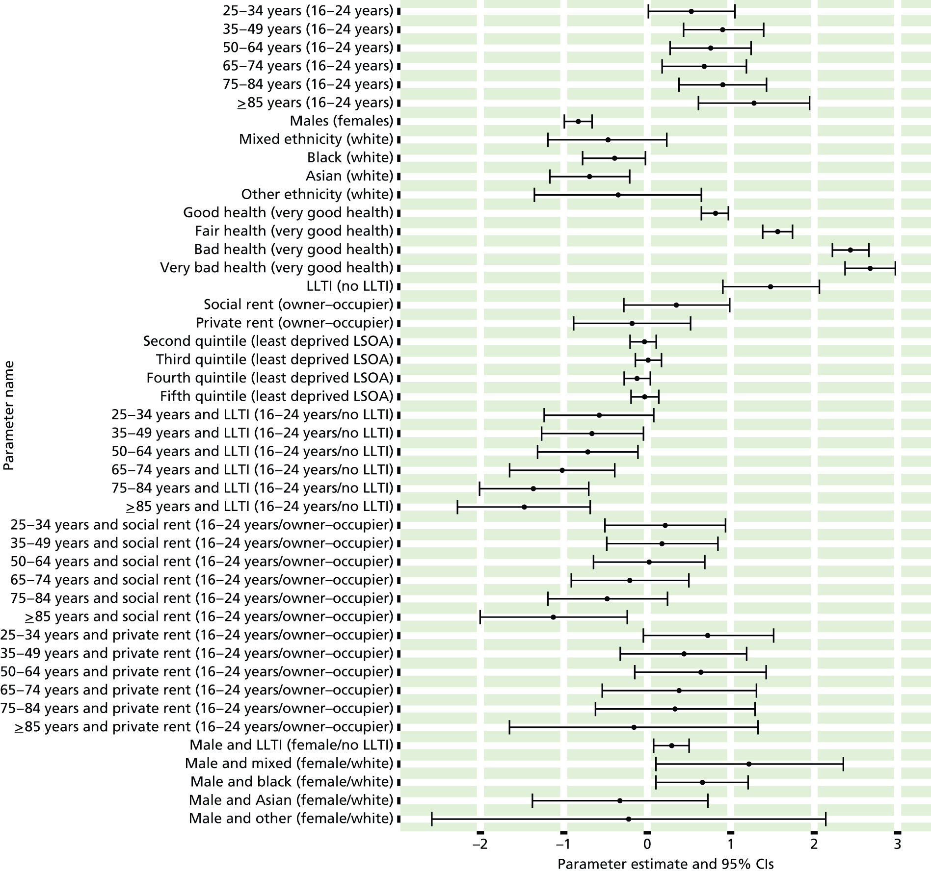
FIGURE 131.
Psychiatric morbidity (HSfE GHQ12 score of ≥ 8) or depression/anxiety drugs: individual estimates and their 95% CIs. (a) MSOAs; (b) LAs; (c) CCGs; and (d) regions (GORs).

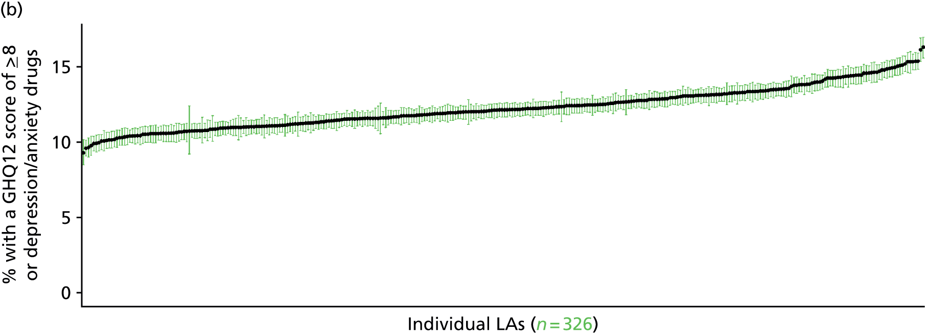
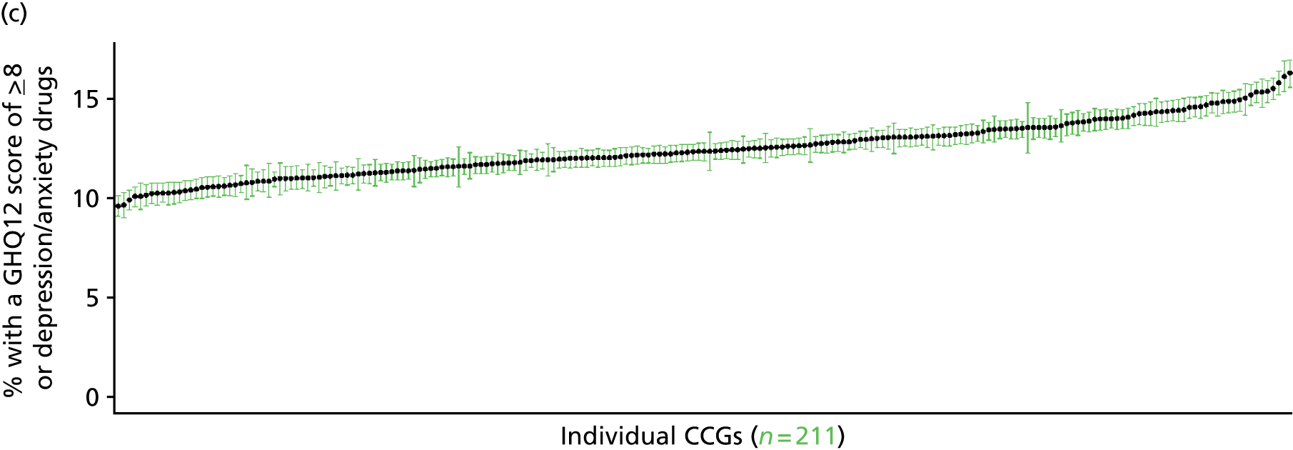
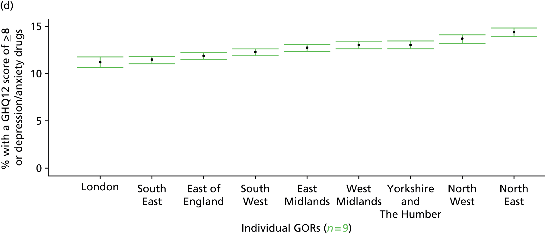
‘Possible’ psychiatric morbidity (12-item General Health Questionnaire score ≥ 4) (UK Household Longitudinal Survey, wave 1, 2009–11)
FIGURE 132.
‘Possible’ psychiatric morbidity (UKHLS wave 1, GHQ12 score of ≥ 4): LSOA-level map. Contains Ordnance Survey data © Crown copyright and database right 2012.

Response variable definition, provenance and prediction
Based on the GHQ12 incorporated within the 2009–11 first wave of the UKHLS, here we capture whether respondents score ≥ 4 using the standard 0–12 ‘caseness’ scoring approach. The GHQ12 is a screening device for identifying minor psychiatric disorders in the general population. It assesses the respondent’s current state and asks if that differs from their usual state. It is sensitive to short-term psychiatric disorders but not long-standing attributes of the respondent. In the literature, a score of ≥ 4 is usually taken as being indicative of ‘possible psychiatric morbidity’. This is not independent of sociodemographic or geographic variations in access to, or uptake of, care as individuals may score < 4 because they are currently being treated for a mental health issue. (See below for an alternative marker which includes people currently being treated with medication for anxiety/depression.)
The first wave of the UKHLS data set (n = 50,994) runs from January 2009 to January 2011 and includes multiple household respondents aged ≥ 16 years from across the UK. Here the analytical data set is drawn from the subset of respondents living in England and for whom data are available across all model response and predictor variables, namely that they completed the GHQ12 questionnaire, along with information on age band, sex, ethnicity, LLTI, tenure and the IMD score of the LSOA of residence (n = 32,903). A single randomly selected adult is then drawn from each household, resulting in an analytical data set of 20,849 adults aged ≥ 16 years.
| Age band (years) | Females | Age band (years) | Males | ||||
|---|---|---|---|---|---|---|---|
| Does not have condition | Has condition | % | Does not have condition | Has condition | % | ||
| 16–24 | 626 | 208 | 24.9 | 16–24 | 469 | 89 | 15.9 |
| 25–34 | 1667 | 455 | 21.4 | 25–34 | 1103 | 247 | 18.3 |
| 35–49 | 3038 | 956 | 23.9 | 35–49 | 2098 | 492 | 19.0 |
| 50–64 | 2261 | 685 | 23.3 | 50–64 | 1921 | 382 | 16.6 |
| 65–74 | 1061 | 185 | 14.8 | 65–74 | 1083 | 129 | 10.6 |
| 75–84 | 613 | 118 | 16.1 | 75–84 | 536 | 99 | 15.6 |
| ≥ 85 | 152 | 45 | 22.8 | ≥ 85 | 109 | 22 | 16.8 |
| Females | 9418 | 2652 | 22.0 | Males | 7319 | 1460 | 16.6 |
| Total (males and females) | 16,737 | 4112 | 19.7 | ||||
Model parameters are applied to microsimulated LSOA-level census data to produce estimates of the number (and proportion) of people with ‘possible psychiatric morbidity (i.e. who would score ≥ 4 on the GHQ12) in each age–sex cohort (and overall) in each of the 32,844 English LSOAs. As discussed in the report, bootstrapping is used to derive 95% CIs for the estimates. These LSOA-level prevalence rate estimates (and 95% CIs) are aggregated into a number of higher geographies, namely MSOAs, LAs, CCGs and regions (GORs). Proportionate attribution is used to restructure the prevalence rate estimates to align with 2001 MSOAs, as well as GP practice populations as defined by the 2011 NHS ADS.
Table 155 summarises how expected prevalence rates vary by age, sex and local deprivation (as measured by the 2010 IMD). There are 6569 LSOAs (with 9,226,227 adults) classified as being in the least deprived quintile; 6568 LSOAs (9,525,344 adults) in the second least deprived quintile; 6568 LSOAs (9,658,444 adults) in the third least deprived quintile; 6568 LSOAs (9,650,576 adults) in the fourth least deprived quintile; and 6568 LSOAs (9,535,167 adults) in the most deprived quintile. Note that, as a general rule, variations in prevalence rates reflect variations in the socioeconomic composition of populations in the different types of LSOA rather than variations in deprivation per se.
| Cohort | Least deprived quintile LSOAs | Second least deprived quintile LSOAs | Third least deprived quintile LSOAs | Fourth least deprived quintile LSOAs | Most deprived quintile LSOAs | All England |
|---|---|---|---|---|---|---|
| Female 16–24 | 17.5 (15.5 to 19.3) | 18.0 (15.9 to 19.8) | 18.5 (16.5 to 20.4) | 19.4 (17.4 to 21.3) | 20.4 (18.4 to 22.5) | 18.9 (16.9 to 20.8) |
| Female 25–34 | 17.8 (16.6 to 19.0) | 18.2 (17.0 to 19.6) | 18.9 (17.7 to 20.3) | 19.8 (18.6 to 21.3) | 21.4 (20.0 to 22.9) | 19.5 (18.3 to 20.9) |
| Female 35–49 | 19.5 (18.4 to 20.7) | 20.3 (19.2 to 21.5) | 21.6 (20.3 to 22.8) | 23.2 (21.9 to 24.5) | 25.9 (24.3 to 27.3) | 22.1 (20.8 to 23.3) |
| Female 50–64 | 18.2 (17.1 to 19.1) | 19.3 (18.1 to 20.2) | 20.7 (19.3 to 21.6) | 22.8 (21.3 to 23.8) | 26.2 (24.3 to 27.3) | 21.2 (19.8 to 22.1) |
| Female 65–74 | 12.9 (11.5 to 14.2) | 13.6 (12.3 to 15.0) | 14.5 (13.1 to 16.1) | 16.1 (14.3 to 17.8) | 18.3 (16.3 to 20.2) | 14.8 (13.3 to 16.4) |
| Female ≥ 75 | 19.4 (17.6 to 21.1) | 20.0 (18.3 to 21.8) | 20.7 (18.9 to 22.5) | 21.8 (19.9 to 23.8) | 23.5 (21.3 to 25.5) | 21.0 (19.1 to 22.8) |
| Females | 17.9 (16.5 to 19.1) | 18.6 (17.2 to 19.9) | 19.6 (18.1 to 21.0) | 21.1 (19.5 to 22.5) | 23.2 (21.4 to 24.8) | 20.1 (18.6 to 21.5) |
| Male 16–24 | 12.8 (11.4 to 14.2) | 13.2 (11.7 to 14.6) | 13.7 (12.2 to 15.2) | 14.4 (12.7 to 15.9) | 15.5 (13.6 to 17.0) | 14.1 (12.4 to 15.6) |
| Male 25–34 | 12.9 (11.8 to 14.2) | 13.2 (12.1 to 14.7) | 13.9 (12.7 to 15.2) | 14.6 (13.4 to 16.1) | 16.0 (14.7 to 17.5) | 14.4 (13.2 to 15.8) |
| Male 35–49 | 14.1 (13.2 to 15.2) | 14.8 (13.9 to 16.0) | 15.7 (14.8 to 17.0) | 17.1 (16.1 to 18.5) | 19.5 (18.2 to 20.9) | 16.3 (15.3 to 17.6) |
| Male 50–64 | 13.1 (12.2 to 14.0) | 14.1 (13.1 to 15.0) | 15.0 (14.1 to 16.1) | 16.8 (15.6 to 17.9) | 19.5 (18.1 to 20.8) | 15.5 (14.5 to 16.5) |
| Male 65–74 | 9.1 (8.1 to 10.0) | 9.8 (8.7 to 10.8) | 10.5 (9.3 to 11.6) | 11.6 (10.3 to 12.8) | 13.3 (11.7 to 14.7) | 10.7 (9.5 to 11.7) |
| Male ≥ 75 | 13.6 (12.1 to 15.2) | 14.2 (12.6 to 15.8) | 14.7 (13.1 to 16.3) | 15.6 (13.9 to 17.3) | 16.9 (15.0 to 18.6) | 14.8 (13.2 to 16.4) |
| Males | 12.8 (11.8 to 14.0) | 13.5 (12.4 to 14.7) | 14.3 (13.1 to 15.5) | 15.5 (14.2 to 16.8) | 17.4 (15.9 to 18.8) | 14.7 (13.5 to 16.0) |
| All | 15.4 (14.9 to 16.0) | 16.1 (15.6 to 16.7) | 17.0 (16.4 to 17.6) | 18.4 (17.6 to 19.0) | 20.4 (19.4 to 21.2) | 17.5 (16.8 to 18.1) |
| Factor (reference group) | Model coefficients | 95% CI | ||
|---|---|---|---|---|
| Estimate | SE | 2.5% CI | 97.50% | |
| (Intercept) | –1.78638 | 0.08784 | –1.95856 | –1.61421 |
| Age (16–24 years) | ||||
| 25–34 years | 0.00019 | 0.08043 | –0.15746 | 0.15784 |
| 35–49 years | 0.07331 | 0.07693 | –0.07748 | 0.22410 |
| 50–64 years | –0.15686 | 0.08174 | –0.31707 | 0.00335 |
| 65–74 years | –0.81339 | 0.09785 | –1.00517 | –0.62161 |
| 75–84 years | –0.71849 | 0.10806 | –0.93029 | –0.50670 |
| ≥ 85 years | –0.48735 | 0.16123 | –0.80336 | –0.17135 |
| Sex (females) | ||||
| Males | –0.39741 | 0.06783 | –0.53035 | –0.26447 |
| Ethnicity (white) | ||||
| Mixed | 0.20351 | 0.12284 | –0.03726 | 0.44428 |
| Black | 0.14654 | 0.06362 | 0.02185 | 0.27124 |
| Asian | –0.12776 | 0.07878 | –0.28216 | 0.02664 |
| Other | 0.25149 | 0.12878 | –0.00092 | 0.50389 |
| LLTI (no LTTI) | ||||
| LLTI | 1.10975 | 0.06920 | 0.97413 | 1.24538 |
| Tenure (owner–occupier) | ||||
| Social rent | 0.46941 | 0.04896 | 0.37344 | 0.56537 |
| Private rent or other tenure | 0.29205 | 0.05223 | 0.18969 | 0.39442 |
| LSOA IMD deprivation score | ||||
| IMD score | 0.00357 | 0.00173 | 0.00019 | 0.00696 |
| Interaction effects | ||||
| Male (female) by LSOA IMD | 0.00396 | 0.00224 | –0.00043 | 0.00836 |
| LLTI (no LLTI) by LSOA IMD score | 0.00392 | 0.00225 | –0.00048 | 0.00832 |
FIGURE 133.
Parameter plots: ‘possible’ psychiatric morbidity (UKHLS wave 1, GHQ12 score of ≥ 4).
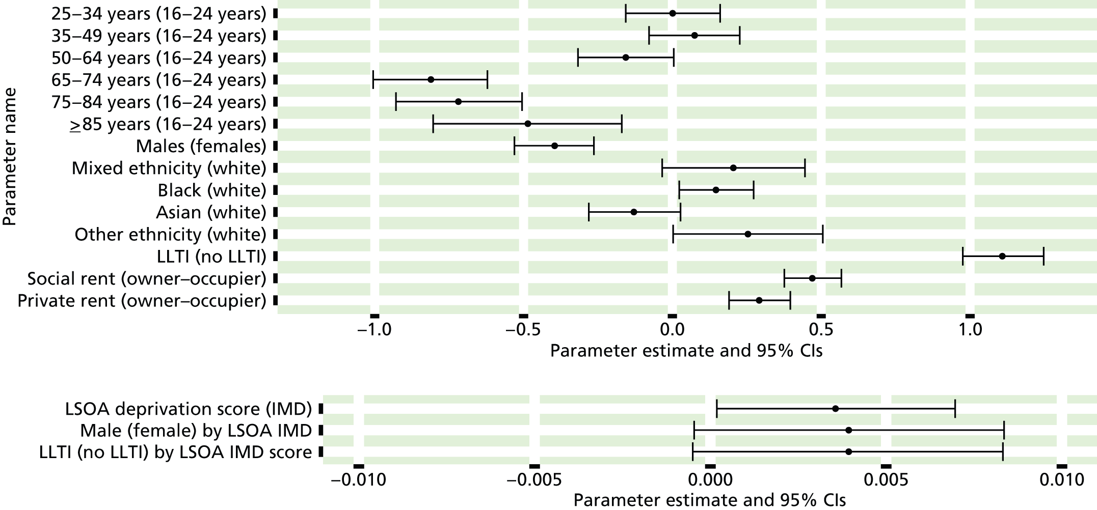
FIGURE 134.
‘Possible’ psychiatric morbidity (UKHLS wave 1, GHQ12 score of ≥ 4): individual estimates and their 95% CIs. (a) MSOAs; (b) LAs; (c) CCGs; and (d) regions (GORs).
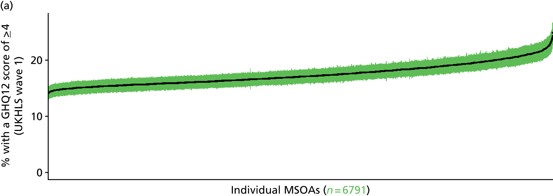

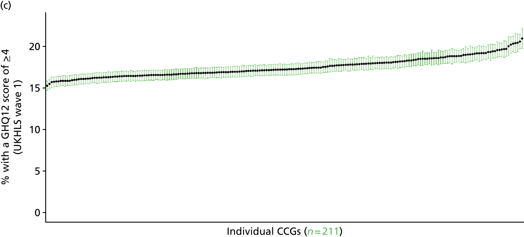
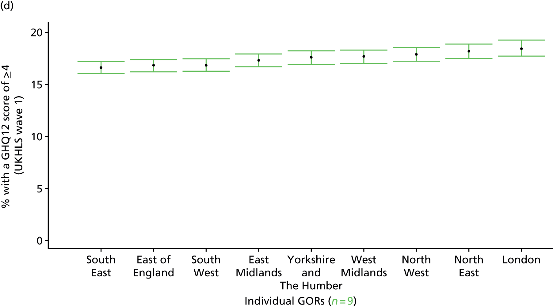
‘Probable’ psychiatric morbidity (12-item General Health Questionnaire score ≥ 6) (UK Household Longitudinal Survey, wave 1, 2009–11)
FIGURE 135.
‘Possible’ psychiatric morbidity (UKHLS wave 1, GHQ12 score of ≥ 6): LSOA-level map. Contains Ordnance Survey data © Crown copyright and database right 2012.
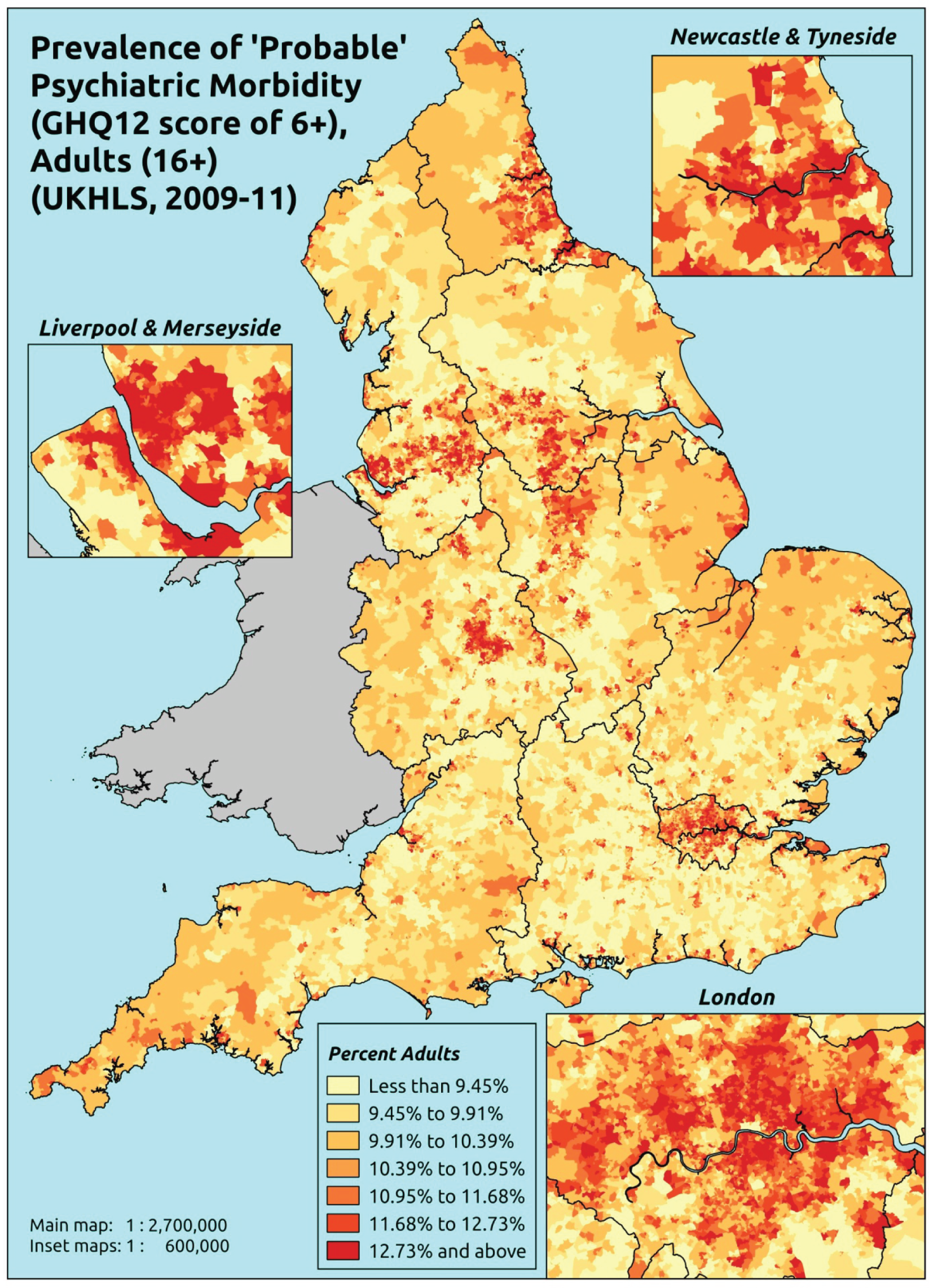
Response variable definition, provenance and prediction
Based on the GHQ12 implemented as part of the 2009–11 first wave of the UKHLS, this captures whether people score ≥ 6 using the standard 0–12 ‘caseness’ scoring approach. The GHQ12 is a screening device for identifying minor psychiatric disorders in the general population. It assesses the respondent’s current state and asks if that differs from their usual state. It is sensitive to short-term psychiatric disorders but not long-standing attributes of the respondent. In the literature, a score of ≥ 4 is usually taken as being indicative of ‘possible psychiatric morbidity’, but occasionally a ≥ 6 threshold is used. For convenience (and without clinical justification) we describe this as a marker of ‘probable psychiatric morbidity’ – to distinguish this marker from those using the standard ≥ 4 threshold (‘possible psychiatric morbidity’) and the higher ≥ 8 threshold (‘psychiatric morbidity’). This is not independent of sociodemographic or geographic variations in access to, or uptake of, care as individuals may score < 6 because they are currently being treated for a mental health issue. (See below for an alternative marker below which includes people currently being treated with medication for anxiety/depression.)
The first wave of the UKHLS data set (n = 50,994) runs from January 2009 to January 2011 and includes multiple household respondents aged ≥ 16 years from across the UK. Here the analytical data set is drawn from the subset of respondents living in England and for whom data is available across all model response and predictor variables, namely that they completed the GHQ12 questionnaire, along with information on age band, sex, ethnicity, LLTI, tenure and the IMD score of the LSOA of residence (n = 32,903). A single randomly selected adult is then drawn from each household, resulting in an analytical data set of 20,849 adults aged ≥ 16 years.
| Age band (years) | Females | Age band (years) | Males | ||||
|---|---|---|---|---|---|---|---|
| Does not have condition | Has condition | % | Does not have condition | Has condition | % | ||
| 16–24 | 712 | 122 | 14.6 | 16–24 | 507 | 51 | 9.1 |
| 25–34 | 1847 | 275 | 13.0 | 25–34 | 1203 | 147 | 10.9 |
| 35–49 | 3331 | 663 | 16.6 | 35–49 | 2263 | 327 | 12.6 |
| 50–64 | 2489 | 457 | 15.5 | 50–64 | 2042 | 261 | 11.3 |
| 65–74 | 1133 | 113 | 9.1 | 65–74 | 1133 | 79 | 6.5 |
| 75–84 | 671 | 60 | 8.2 | 75–84 | 574 | 61 | 9.6 |
| ≥ 85 | 168 | 29 | 14.7 | ≥ 85 | 119 | 12 | 9.2 |
| Females | 10,351 | 1719 | 14.2 | Males | 7841 | 938 | 10.7 |
| Total (males and females) | 18,192 | 2657 | 12.7 | ||||
Model parameters are applied to microsimulated LSOA-level census data to produce estimates of the number (and proportion) of people with ‘probable psychiatric morbidity (i.e. who would score ≥ 6 on the GHQ12) in each age–sex cohort (and overall) in each of the 32,844 English LSOAs. As discussed in the report, bootstrapping is used to derive 95% CIs for the estimates. These LSOA-level prevalence rate estimates (and 95% CIs) are aggregated into a number of higher geographies, namely MSOAs, LAs, CCGs and regions (GORs). Proportionate attribution is used to restructure the prevalence rate estimates to align with 2001 MSOAs, as well as GP practice populations as defined by the 2011 NHS ADS.
Table 158 summarises how expected prevalence rates vary by age, sex and local deprivation (as measured by the 2010 IMD). There are 6569 LSOAs (with 9,226,227 adults) classified as being in the least deprived quintile; 6568 LSOAs (9,525,344 adults) in the second least deprived quintile; 6568 LSOAs (9,658,444 adults) in the third least deprived quintile; 6568 LSOAs (9,650,576 adults) in the fourth least deprived quintile; and 6568 LSOAs (9,535,167 adults) in the most deprived quintile. Note that, as a general rule, variations in prevalence rates reflect variations in the socioeconomic composition of populations in the different types of LSOA rather than variations in deprivation per se.
| Cohort | Least deprived quintile LSOAs | Second least deprived quintile LSOAs | Third least deprived quintile LSOAs | Fourth least deprived quintile LSOAs | Most deprived quintile LSOAs | All England |
|---|---|---|---|---|---|---|
| Female 16–24 | 9.8 (8.6 to 11.1) | 10.1 (8.9 to 11.5) | 10.5 (9.2 to 12.0) | 11.1 (9.7 to 12.6) | 11.9 (10.3 to 13.5) | 10.8 (9.4 to 12.3) |
| Female 25–34 | 10.4 (9.3 to 11.1) | 10.8 (9.6 to 11.5) | 11.2 (10.1 to 12.0) | 11.9 (10.7 to 12.7) | 13.0 (11.8 to 13.9) | 11.7 (10.5 to 12.4) |
| Female 35–49 | 12.9 (12.1 to 13.9) | 13.6 (12.8 to 14.7) | 14.6 (13.7 to 15.6) | 16.0 (15.1 to 17.1) | 18.2 (17.1 to 19.5) | 15.1 (14.2 to 16.1) |
| Female 50–64 | 12.0 (11.1 to 12.9) | 12.9 (12.0 to 13.9) | 14.0 (13.0 to 15.0) | 15.7 (14.6 to 16.8) | 18.4 (17.1 to 19.8) | 14.4 (13.4 to 15.5) |
| Female 65–74 | 7.9 (6.7 to 8.9) | 8.5 (7.2 to 9.6) | 9.1 (7.8 to 10.3) | 10.2 (8.7 to 11.5) | 11.8 (10.1 to 13.3) | 9.3 (7.9 to 10.5) |
| Female ≥ 75 | 11.4 (9.7 to 12.9) | 11.9 (10.2 to 13.4) | 12.4 (10.7 to 14.0) | 13.2 (11.3 to 14.9) | 14.3 (12.3 to 16.2) | 12.5 (10.8 to 14.1) |
| Females | 11.2 (10.1 to 12.3) | 11.8 (10.7 to 12.9) | 12.5 (11.3 to 13.6) | 13.6 (12.3 to 14.8) | 15.2 (13.8 to 16.6) | 12.9 (11.7 to 14.0) |
| Male 16–24 | 6.6 (5.8 to 7.6) | 6.8 (6.0 to 7.9) | 7.1 (6.3 to 8.3) | 7.6 (6.7 to 8.7) | 8.2 (7.3 to 9.5) | 7.3 (6.5 to 8.5) |
| Male 25–34 | 6.9 (6.0 to 7.6) | 7.2 (6.3 to 8.0) | 7.6 (6.7 to 8.4) | 8.1 (7.1 to 9.0) | 9.0 (8.1 to 10.0) | 7.9 (7.0 to 8.8) |
| Male 35–49 | 8.6 (7.8 to 9.5) | 9.1 (8.4 to 10.2) | 9.9 (9.1 to 11.0) | 11.1 (10.2 to 12.2) | 12.9 (12.0 to 14.3) | 10.3 (9.5 to 11.5) |
| Male 50–64 | 8.0 (7.5 to 8.9) | 8.8 (8.2 to 9.8) | 9.7 (9.1 to 10.8) | 11.1 (10.4 to 12.3) | 13.4 (12.5 to 14.8) | 10.1 (9.4 to 11.2) |
| Male 65–74 | 5.4 (4.7 to 6.2) | 5.9 (5.1 to 6.8) | 6.4 (5.5 to 7.5) | 7.3 (6.3 to 8.4) | 8.5 (7.4 to 9.9) | 6.6 (5.7 to 7.6) |
| Male ≥ 75 | 7.8 (6.9 to 9.2) | 8.3 (7.2 to 9.7) | 8.6 (7.6 to 10.2) | 9.2 (8.2 to 10.9) | 10.2 (9.0 to 12.0) | 8.7 (7.7 to 10.3) |
| Males | 7.5 (6.8 to 8.5) | 8.0 (7.2 to 9.0) | 8.6 (7.8 to 9.7) | 9.4 (8.6 to 10.6) | 10.8 (9.9 to 12.2) | 8.9 (8.1 to 10.0) |
| All | 9.4 (9.1 to 9.9) | 10.0 (9.6 to 10.5) | 10.6 (10.2 to 11.2) | 11.6 (11.1 to 12.2) | 13.1 (12.5 to 13.8) | 10.9 (10.5 to 11.5) |
| Factor (reference group) | Model coefficients | 95% CI | ||
|---|---|---|---|---|
| Estimate | SE | 2.5% CI | 97.50% | |
| (Intercept) | –2.52055 | 0.10351 | –2.72343 | –2.31766 |
| Age (16–24 years) | ||||
| 25–34 years | 0.04674 | 0.09911 | –0.14752 | 0.24100 |
| 35–49 years | 0.25323 | 0.09350 | 0.06996 | 0.43650 |
| 50–64 years | 0.00093 | 0.09895 | –0.19301 | 0.19487 |
| 65–74 years | –0.72443 | 0.11997 | –0.95957 | –0.48929 |
| 75–84 years | –0.75722 | 0.13469 | –1.02121 | –0.49323 |
| ≥ 85 years | –0.45101 | 0.19511 | –0.83342 | –0.06861 |
| Sex (females) | ||||
| Males | –0.52028 | 0.09027 | –0.69721 | –0.34334 |
| Ethnicity (white) | ||||
| Mixed | 0.51292 | 0.22535 | 0.07124 | 0.95460 |
| Black | 0.29177 | 0.09853 | 0.09865 | 0.48489 |
| Asian | –0.15536 | 0.18130 | –0.51070 | 0.19998 |
| Other | 0.46520 | 0.23902 | –0.00327 | 0.93367 |
| LLTI (no LTTI) | ||||
| LLTI | 1.21390 | 0.05722 | 1.10175 | 1.32606 |
| Tenure (owner–occupier) | ||||
| Social rent | 0.54350 | 0.06276 | 0.42049 | 0.66651 |
| Private rent or other tenure | 0.42325 | 0.07004 | 0.28596 | 0.56054 |
| LSOA IMD deprivation score | ||||
| IMD score | 0.00410 | 0.00174 | 0.00068 | 0.00751 |
| Interaction effects | ||||
| Male by LSOA IMD | 0.00726 | 0.00263 | 0.00211 | 0.01241 |
| Mixed and social rent | –0.40292 | 0.32153 | –1.03312 | 0.22728 |
| Black and social rent | –0.48702 | 0.19078 | –0.86095 | –0.11310 |
| Asian and social rent | 0.01306 | 0.22098 | –0.42005 | 0.44618 |
| Other and social rent | 0.02364 | 0.34254 | –0.64774 | 0.69503 |
| Mixed and private rent | –0.41264 | 0.35262 | –1.10378 | 0.27850 |
| Black and private rent | –0.44307 | 0.17987 | –0.79561 | –0.09052 |
| Asian and private rent | –0.29042 | 0.27702 | –0.83338 | 0.25254 |
| Other and private rent | –0.67463 | 0.38023 | –1.41989 | 0.07062 |
| Male and LLTI | 0.13733 | 0.09060 | –0.04024 | 0.31491 |
FIGURE 136.
Parameter plots: ‘possible’ psychiatric morbidity (UKHLS wave 1, GHQ12 score of ≥ 6).
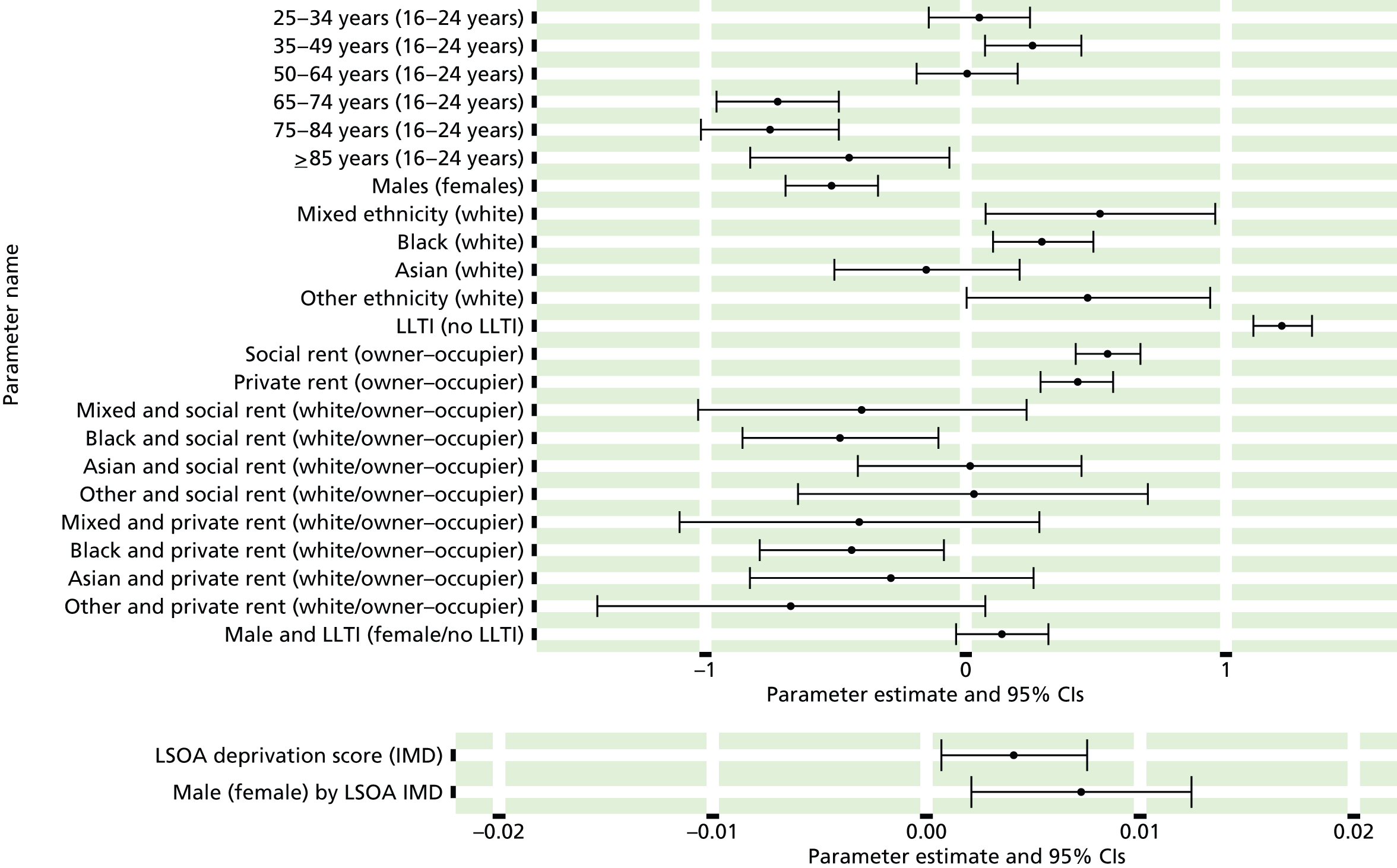
FIGURE 137.
‘Possible’ psychiatric morbidity (UKHLS wave 1, GHQ12 score of ≥ 6): individual estimates and their 95% CIs. (a) MSOAs; (b) LAs; (c) CCGs; and (d) regions (GORs).

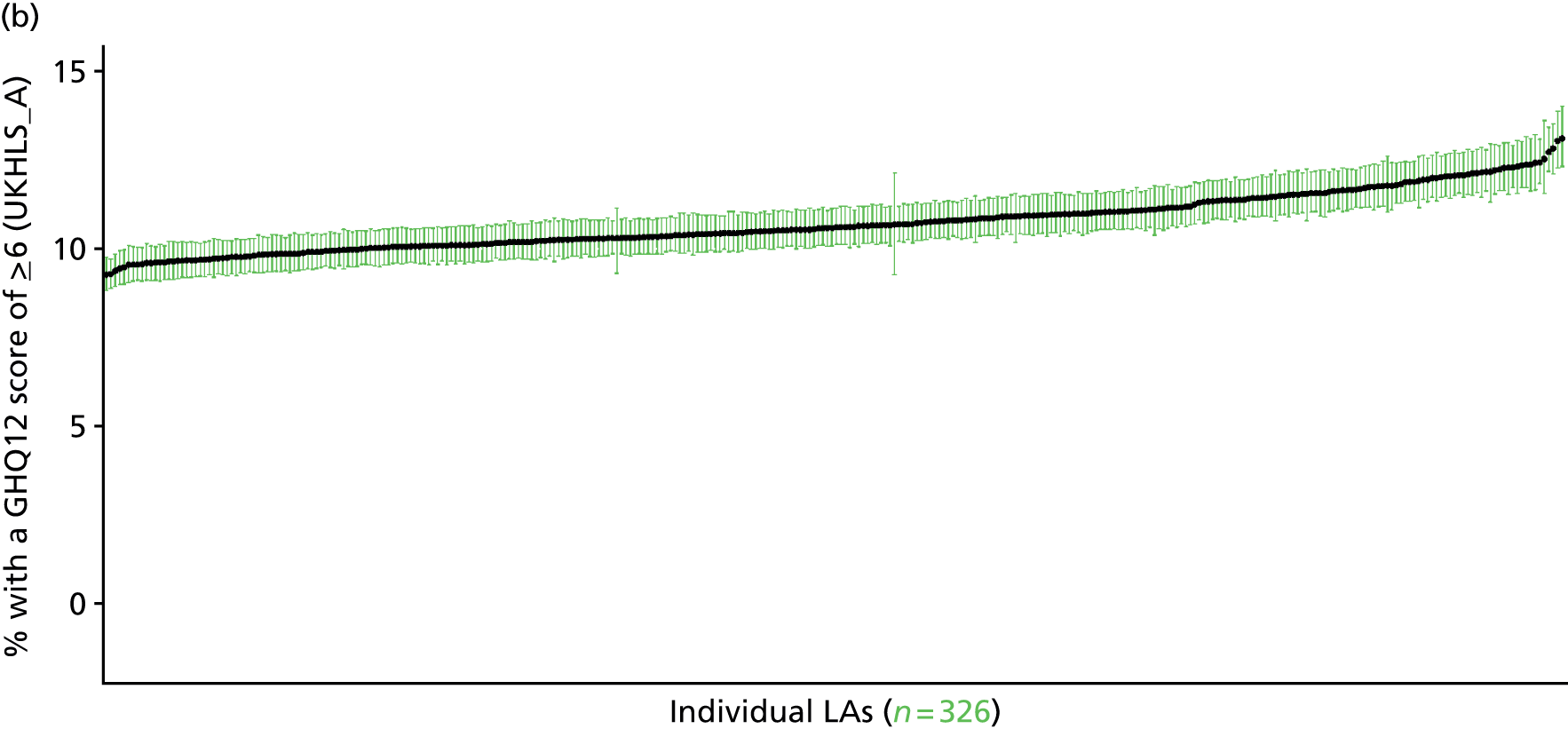
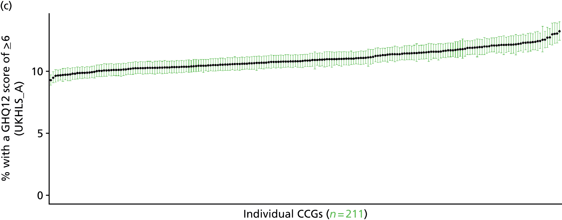

Psychiatric morbidity (12-item General Health Questionnaire score ≥ 8) (UK Household Longitudinal Survey, wave 1, 2009–11)
FIGURE 138.
‘Possible’ psychiatric morbidity (UKHLS wave 1, GHQ12 score of ≥ 8): LSOA-level map. Contains Ordnance Survey data © Crown copyright and database right 2012.

Response variable definition, provenance and prediction
Based on the GHQ12 implemented as part of the 2009–11 first wave of the UKHLS, here we capture whether or not people score ≥ 8 using the standard 0–12 ‘caseness’ scoring approach. The GHQ12 is a screening device for identifying minor psychiatric disorders in the general population. It assesses the respondent’s current state and asks if that differs from his or her usual state. It is sensitive to short-term psychiatric disorders but not to long-standing attributes of the respondent. In the literature, a score of ≥ 4 is usually taken as being indicative of ‘possible psychiatric morbidity’, but occasionally ≥ 6 or ≥ 8 thresholds are used. For convenience (and without clinical justification) we describe a score of ≥ 8 as being indicative of ‘psychiatric morbidity’ – to distinguish it from the standard ≥ 4 threshold (‘possible psychiatric morbidity’) and the ≥ 6 threshold (‘probable psychiatric morbidity’). This is not independent of sociodemographic or geographic variations in access to, or uptake of, care, as individuals may score < 8 because they are currently being treated for a mental health issue. (See below for an alternative marker below which includes people currently being treated with medication for anxiety/depression.)
The first wave of the UKHLS data set (n = 50,994) runs from January 2009 to January 2011 and includes multiple household respondents aged ≥ 16 from across the UK. Here the analytical data set is drawn from the subset of respondents living in England and for whom data are available across all model response and predictor variables, namely that they completed the GHQ12 questionnaire, along with information on age band, sex, ethnicity, LLTI, tenure and the IMD score of the LSOA of residence (n = 32,903). A single randomly selected adult is then drawn from each household, resulting in an analytical data set of 20,849 adults aged ≥ 16 years.
| Age band (years) | Females | Age band (years) | Males | ||||
|---|---|---|---|---|---|---|---|
| Does not have condition | Has condition | % | Does not have condition | Has condition | % | ||
| 16–24 | 766 | 68 | 8.2 | 16–24 | 536 | 22 | 3.9 |
| 25–34 | 1961 | 161 | 7.6 | 25–34 | 1267 | 83 | 6.1 |
| 35–49 | 3563 | 431 | 10.8 | 35–49 | 2366 | 224 | 8.6 |
| 50–64 | 2637 | 309 | 10.5 | 50–64 | 2120 | 183 | 7.9 |
| 65–74 | 1187 | 59 | 4.7 | 65–74 | 1165 | 47 | 3.9 |
| 75–84 | 707 | 24 | 3.3 | 75–84 | 598 | 37 | 5.8 |
| ≥ 85 | 181 | 16 | 8.1 | ≥ 85 | 124 | 7 | 5.3 |
| Females | 11,002 | 1068 | 8.8 | Males | 8176 | 603 | 6.9 |
| Total (males and females) | 19,178 | 1671 | 8.0 | ||||
Model parameters are applied to microsimulated LSOA-level census data to produce estimates of the number (and proportion) of people with ‘psychiatric morbidity (i.e. who would score ≥ 8 on the GHQ12) in each age–sex cohort (and overall) in each of the 32,844 English LSOAs. As discussed in the report, bootstrapping is used to derive 95% CIs for the estimates. These LSOA-level prevalence rate estimates (and 95% CIs) are aggregated into a number of higher geographies; namely MSOAs, LAs, CCGs and regions (GORs). Proportionate attribution is used to restructure the prevalence rate estimates to align with 2001 MSOAs, as well as GP practice populations as defined by the 2011 NHS ADS.
Table 161 summarises how expected prevalence rates vary by age, sex and local deprivation (as measured by the 2010 IMD). There are 6569 LSOAs (with 9,226,227 adults) classified as being in the least deprived quintile; 6568 LSOAs (9,525,344 adults) in the second least deprived quintile; 6568 LSOAs (9,658,444 adults) in the third least deprived quintile; 6568 LSOAs (9,650,576 adults) in the fourth least deprived quintile; and 6568 LSOAs (9,535,167 adults) in the most deprived quintile. Note that, as a general rule, variations in prevalence rates reflect variations in the socioeconomic composition of populations in the different types of LSOA rather than variations in deprivation per se.
| Cohort | Least deprived quintile LSOAs | Second least deprived quintile LSOAs | Third least deprived quintile LSOAs | Fourth least deprived quintile LSOAs | Most deprived quintile LSOAs | All England |
|---|---|---|---|---|---|---|
| Female 16–24 | 5.0 (4.2 to 5.9) | 5.2 (4.4 to 6.1) | 5.4 (4.5 to 6.3) | 5.6 (4.7 to 6.7) | 6.0 (5.0 to 7.2) | 5.5 (4.6 to 6.5) |
| Female 25–34 | 5.9 (5.1 to 6.6) | 6.0 (5.3 to 6.8) | 6.3 (5.6 to 7.1) | 6.7 (6.0 to 7.5) | 7.3 (6.5 to 8.3) | 6.5 (5.8 to 7.4) |
| Female 35–49 | 8.0 (7.4 to 8.8) | 8.6 (7.9 to 9.3) | 9.2 (8.5 to 10.0) | 10.2 (9.3 to 11.0) | 11.7 (10.8 to 12.7) | 9.5 (8.7 to 10.4) |
| Female 50–64 | 7.6 (6.8 to 8.3) | 8.2 (7.4 to 9.0) | 9.0 (8.1 to 9.8) | 10.2 (9.2 to 11.1) | 12.1 (10.9 to 13.2) | 9.3 (8.4 to 10.1) |
| Female 65–74 | 4.0 (3.3 to 4.6) | 4.3 (3.5 to 5.0) | 4.7 (3.8 to 5.4) | 5.3 (4.2 to 6.1) | 6.1 (4.9 to 7.1) | 4.8 (3.9 to 5.5) |
| Female ≥ 75 | 5.6 (4.6 to 6.7) | 5.9 (4.8 to 7.0) | 6.1 (5.0 to 7.3) | 6.5 (5.3 to 7.8) | 7.2 (5.8 to 8.4) | 6.2 (5.1 to 7.3) |
| Females | 6.5 (5.8 to 7.3) | 6.8 (6.1 to 7.7) | 7.3 (6.5 to 8.2) | 8.0 (7.0 to 8.9) | 9.0 (8.0 to 10.1) | 7.5 (6.7 to 8.4) |
| Male 16–24 | 3.2 (2.7 to 3.9) | 3.3 (2.8 to 4.0) | 3.5 (2.9 to 4.2) | 3.7 (3.1 to 4.5) | 4.1 (3.5 to 4.9) | 3.6 (3.1 to 4.3) |
| Male 25–34 | 3.8 (3.3 to 4.3) | 3.9 (3.4 to 4.5) | 4.1 (3.6 to 4.7) | 4.4 (3.9 to 5.0) | 5.1 (4.4 to 5.7) | 4.4 (3.8 to 4.9) |
| Male 35–49 | 5.2 (4.6 to 5.8) | 5.7 (5.1 to 6.3) | 6.2 (5.6 to 6.9) | 7.1 (6.3 to 7.8) | 8.6 (7.7 to 9.5) | 6.6 (5.9 to 7.2) |
| Male 50–64 | 5.2 (4.6 to 5.7) | 5.8 (5.2 to 6.4) | 6.5 (5.8 to 7.2) | 7.6 (6.8 to 8.3) | 9.4 (8.4 to 10.3) | 6.8 (6.1 to 7.5) |
| Male 65–74 | 3.0 (2.4 to 3.5) | 3.3 (2.7 to 3.8) | 3.6 (2.9 to 4.2) | 4.2 (3.3 to 4.8) | 4.9 (4.0 to 5.8) | 3.7 (3.0 to 4.3) |
| Male ≥ 75 | 4.3 (3.5 to 5.2) | 4.5 (3.7 to 5.5) | 4.8 (3.9 to 5.8) | 5.1 (4.2 to 6.2) | 5.5 (4.6 to 6.8) | 4.8 (3.9 to 5.8) |
| Males | 4.4 (3.8 to 5.0) | 4.8 (4.1 to 5.4) | 5.1 (4.5 to 5.8) | 5.7 (5.0 to 6.4) | 6.7 (5.9 to 7.6) | 5.4 (4.7 to 6.0) |
| All | 5.5 (5.2 to 5.8) | 5.8 (5.5 to 6.2) | 6.3 (5.9 to 6.7) | 6.9 (6.5 to 7.3) | 7.9 (7.4 to 8.5) | 6.5 (6.1 to 6.9) |
| Factor (reference group) | Model coefficients | 95% CI | ||
|---|---|---|---|---|
| Estimate | SE | 2.5% CI | 97.50% | |
| (Intercept) | –3.27198 | 0.13451 | –3.53561 | –3.00835 |
| Age (16–24 years) | ||||
| 25–34 years | 0.14697 | 0.13075 | –0.10930 | 0.40324 |
| 35–49 years | 0.44260 | 0.12241 | 0.20267 | 0.68253 |
| 50–64 years | 0.18735 | 0.12808 | –0.06369 | 0.43839 |
| 65–74 years | –0.76187 | 0.15750 | –1.07056 | –0.45317 |
| 75–84 years | –0.91148 | 0.18028 | –1.26483 | –0.55813 |
| ≥ 85 years | –0.50382 | 0.25155 | –0.99686 | –0.01077 |
| Sex (females) | ||||
| Males | –0.59383 | 0.11488 | –0.81899 | –0.36866 |
| Ethnicity (white) | ||||
| Mixed | 0.34767 | 0.28430 | –0.20955 | 0.90489 |
| Black | 0.29873 | 0.11896 | 0.06556 | 0.53189 |
| Asian | –0.27856 | 0.23700 | –0.74309 | 0.18596 |
| Other | 0.45982 | 0.29100 | –0.11054 | 1.03018 |
| LLTI (no LTTI) | ||||
| LLTI | 1.30315 | 0.06908 | 1.16775 | 1.43854 |
| Tenure (owner–occupier) | ||||
| Social rent | 0.52627 | 0.07492 | 0.37942 | 0.67313 |
| Private rent or other tenure | 0.38943 | 0.08588 | 0.22111 | 0.55775 |
| LSOA IMD deprivation score | ||||
| IMD score | 0.00579 | 0.00210 | 0.00167 | 0.00991 |
| Interaction effects | ||||
| Male and LLTI | 0.36439 | 0.11068 | 0.14746 | 0.58132 |
| Male by LSOA IMD | 0.00775 | 0.00317 | 0.00154 | 0.01397 |
| Mixed and social rent | –0.37794 | 0.40085 | –1.16361 | 0.40772 |
| Black and social rent | –0.56026 | 0.23139 | –1.01378 | –0.10673 |
| Asian and social rent | –0.07937 | 0.28594 | –0.63980 | 0.48107 |
| Other and social rent | –0.32572 | 0.41940 | –1.14774 | 0.49631 |
| Mixed and private rent | –0.14362 | 0.43024 | –0.98689 | 0.69964 |
| Black and private rent | –0.75558 | 0.24540 | –1.23658 | –0.27459 |
| Asian and private rent | –0.28624 | 0.36505 | –1.00173 | 0.42926 |
| Other and private rent | –1.04429 | 0.52063 | –2.06473 | –0.02385 |
FIGURE 139.
Parameter plots: ‘possible’ psychiatric morbidity (UKHLS wave 1, GHQ12 score of ≥ 8).
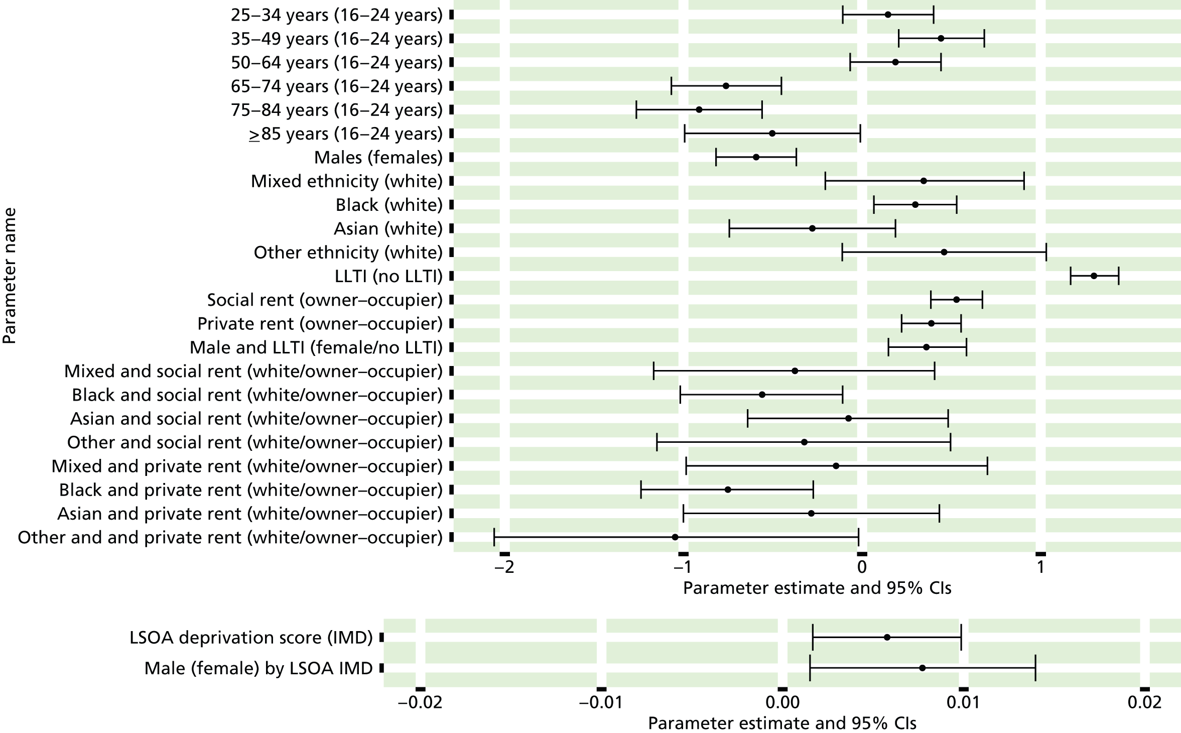
FIGURE 140.
‘Possible’ psychiatric morbidity (UKHLS wave 1, GHQ12 score of ≥ 8): individual estimates and their 95% CIs. (a) MSOAs; (b) LAs; (c) CCGs; and (d) regions (GORs).

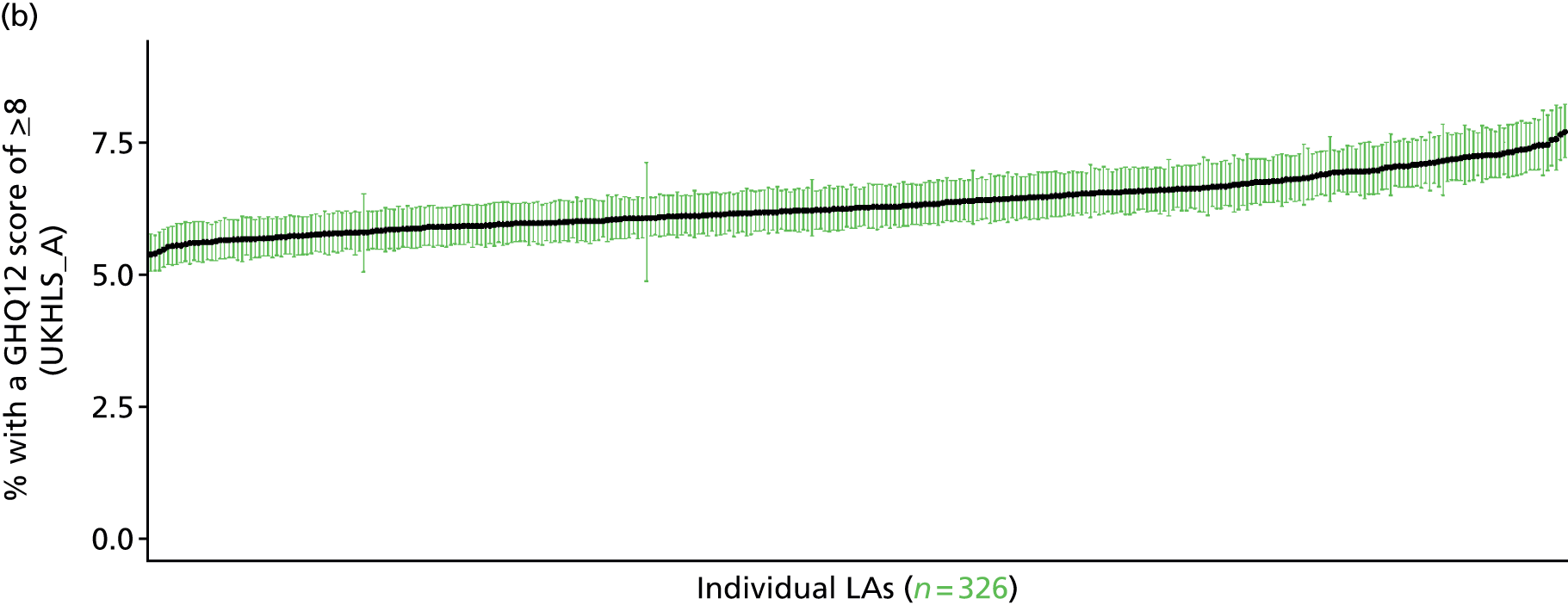

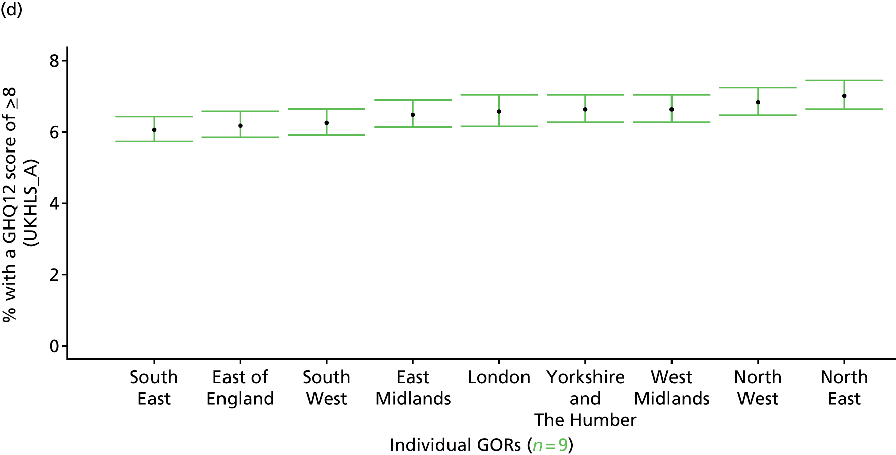
‘Possible’ psychiatric morbidity (12-item General Health Questionnaire score ≥ 4) or currently prescribed depression/anxiety drugs (UK Household Longitudinal Survey, wave 1, 2009–11)
FIGURE 141.
‘Possible’ psychiatric morbidity (UKHLS wave 1, GHQ12 score of ≥ 4) or depression/anxiety drugs: LSOA-level map. Contains Ordnance Survey data © Crown copyright and database right 2012.
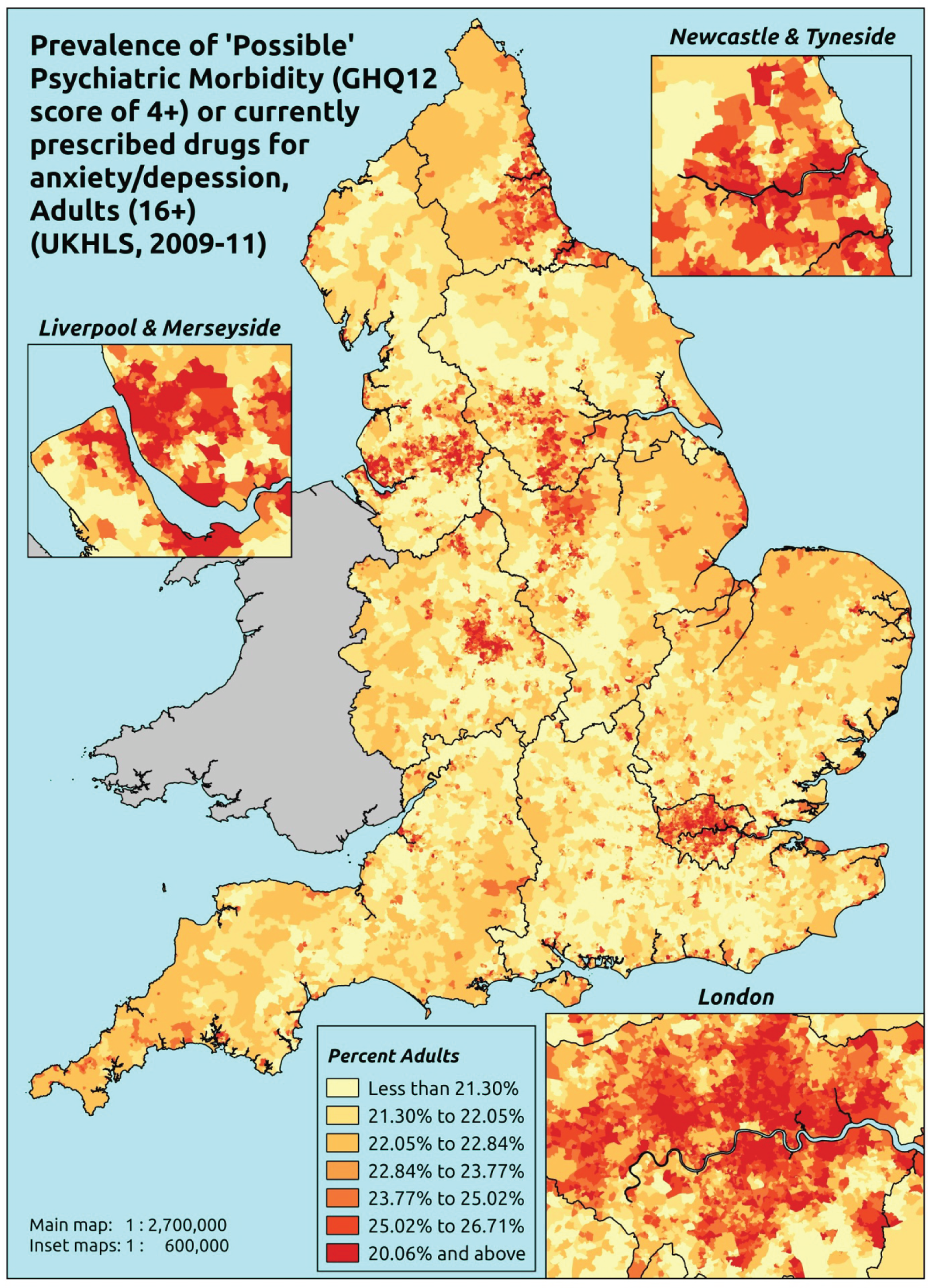
Response variable definition, provenance and prediction
This marker of mental health needs is derived from the 2009–11 first wave of the UKHLS GHQ12 questionnaire score and questions about what medicines the respondent is currently being prescribed, this marker captures respondents with a GHQ12 score of ≥ 4 using the standard 0–12 ‘caseness’ scoring approach and/or who are currently being prescribed drugs for depression and/or anxiety (BNF 4.1.1–4.1.3 or 4.3.1–4.3.4487). In the literature, a score of ≥ 4 is usually taken as being indicative of ‘possible psychiatric morbidity’. We have no information regarding other forms of treatment for mental health issues. This recognises the fact that individuals may return a GHQ12 score of < 4 because they are being receiving medication for anxiety/depression and thus aims to capture underlying levels of ‘possible psychiatric morbidity’. This marker is affected by the fact that (a) other types of medication, and other forms of treatment, are not captured, and (b) any sociodemographic and/or geographic variations in access to, or uptake of, prescribing will affect rates of prescribing and thus this statistic.
The first wave of the UKHLS data set (n = 50,994) runs from January 2009 to January 2011 and includes multiple household respondents aged ≥ 16 years from across the UK. Here the analytical data set is drawn from the subset of respondents living in England and for whom data are available across all model response and predictor variables, namely that they completed the GHQ12 questionnaire and we know what medication they were currently being prescribed, along with information on age band, sex, ethnicity, LLTI, tenure and the IMD score of the LSOA of residence (n = 12,113). A single randomly selected adult is then drawn from each household, resulting in an analytical data set of 8340 adults aged ≥ 16 years.
| Age band (years) | Females | Age band (years) | Males | ||||
|---|---|---|---|---|---|---|---|
| Does not have condition | Has condition | % | Does not have condition | Has condition | % | ||
| 16–24 | 149 | 52 | 25.9 | 16–24 | 86 | 20 | 18.9 |
| 25–34 | 460 | 196 | 29.9 | 25–34 | 315 | 79 | 20.1 |
| 35–49 | 1075 | 503 | 31.9 | 35–49 | 689 | 226 | 24.7 |
| 50–64 | 941 | 480 | 33.8 | 50–64 | 845 | 226 | 21.1 |
| 65–74 | 488 | 138 | 22.0 | 65–74 | 512 | 85 | 14.2 |
| 75–84 | 263 | 79 | 23.1 | 75–84 | 241 | 62 | 20.5 |
| ≥ 85 | 45 | 23 | 33.8 | ≥ 85 | 49 | 13 | 21.0 |
| Females | 3421 | 1471 | 30.1 | Males | 2737 | 711 | 20.6 |
| Total (males and females) | 6158 | 2182 | 26.2 | ||||
Model parameters are applied to microsimulated LSOA-level census data to produce estimates of the number (and proportion) of people with treated or untreated ‘possible psychiatric morbidity (i.e. who would score ≥ 4 on the GHQ12 or be currently prescribed drugs for depression and/or anxiety) in each age–sex cohort (and overall) in each of the 32,844 English LSOAs. As discussed in the report, bootstrapping is used to derive 95% CIs for the estimates. These LSOA-level prevalence rate estimates (and 95% CIs) are aggregated into a number of higher geographies; namely MSOAs, LAs, CCGs and regions (GORs). Proportionate attribution is used to restructure the prevalence rate estimates to align with 2001 MSOAs, as well as GP practice populations as defined by the 2011 NHS ADS.
Table 164 summarises how expected prevalence rates vary by age, sex and local deprivation (as measured by the 2010 IMD). There are 6569 LSOAs (with 9,226,227 adults) classified as being in the least deprived quintile; 6568 LSOAs (9,525,344 adults) in the second least deprived quintile; 6568 LSOAs (9,658,444 adults) in the third least deprived quintile; 6568 LSOAs (9,650,576 adults) in the fourth least deprived quintile; and 6568 LSOAs (9,535,167 adults) in the most deprived quintile. Note that, as a general rule, variations in prevalence rates reflect variations in the socioeconomic composition of populations in the different types of LSOA rather than variations in deprivation per se.
| Cohort | Least deprived quintile LSOAs | Second least deprived quintile LSOAs | Third least deprived quintile LSOAs | Fourth least deprived quintile LSOAs | Most deprived quintile LSOAs | All England |
|---|---|---|---|---|---|---|
| Female 16–24 | 20.5 (16.3 to 24.4) | 21.0 (16.8 to 25.1) | 21.6 (17.5 to 25.8) | 22.5 (18.4 to 26.9) | 23.8 (19.6 to 28.6) | 22.1 (18.0 to 26.4) |
| Female 25–34 | 26.2 (23.5 to 28.5) | 26.7 (24.3 to 29.3) | 27.6 (25.1 to 30.4) | 28.9 (26.3 to 31.8) | 30.9 (28.3 to 34.0) | 28.4 (25.9 to 31.2) |
| Female 35–49 | 28.7 (27.0 to 30.5) | 29.8 (28.1 to 31.6) | 31.1 (29.5 to 33.0) | 33.1 (31.6 to 35.3) | 36.4 (34.7 to 38.9) | 31.8 (30.2 to 33.8) |
| Female 50–64 | 27.5 (25.5 to 29.3) | 28.8 (26.8 to 30.8) | 30.4 (28.5 to 32.7) | 33.1 (31.2 to 35.5) | 37.3 (35.2 to 40.1) | 31.1 (29.1 to 33.3) |
| Female 65–74 | 20.4 (18.4 to 21.9) | 21.5 (19.5 to 23.1) | 22.7 (20.6 to 24.6) | 24.8 (22.6 to 27.0) | 27.9 (25.6 to 30.4) | 23.1 (21.0 to 25.0) |
| Female ≥ 75 | 28.8 (26.1 to 31.9) | 29.8 (26.9 to 33.0) | 30.9 (27.8 to 34.1) | 32.3 (29.1 to 35.9) | 34.4 (31.1 to 38.2) | 31.1 (28.0 to 34.5) |
| Females | 26.2 (23.9 to 28.4) | 27.1 (24.8 to 29.5) | 28.2 (25.8 to 30.8) | 29.9 (27.5 to 32.7) | 32.5 (29.9 to 35.7) | 28.8 (26.4 to 31.4) |
| Male 16–24 | 12.6 (9.9 to 14.9) | 13.0 (10.2 to 15.4) | 13.5 (10.7 to 16.0) | 14.3 (11.3 to 17.0) | 15.4 (12.3 to 18.5) | 13.9 (11.0 to 16.5) |
| Male 25–34 | 16.5 (14.5 to 18.1) | 17.1 (15.0 to 18.7) | 17.7 (15.7 to 19.4) | 18.7 (16.6 to 20.6) | 20.5 (18.4 to 22.6) | 18.4 (16.3 to 20.2) |
| Male 35–49 | 18.2 (16.4 to 19.9) | 19.1 (17.3 to 20.9) | 20.2 (18.3 to 22.0) | 21.8 (20.1 to 23.9) | 24.6 (22.8 to 26.9) | 20.8 (19.0 to 22.8) |
| Male 50–64 | 17.3 (15.8 to 18.8) | 18.5 (16.9 to 19.9) | 19.8 (18.1 to 21.4) | 21.8 (20.0 to 23.8) | 25.0 (23.2 to 27.2) | 20.3 (18.6 to 22.0) |
| Male 65–74 | 12.5 (11.0 to 13.6) | 13.3 (11.8 to 14.5) | 14.3 (12.6 to 15.6) | 15.7 (14.0 to 17.3) | 17.9 (16.1 to 19.8) | 14.5 (12.8 to 15.9) |
| Male ≥ 75 | 17.9 (15.8 to 20.0) | 18.6 (16.4 to 20.8) | 19.3 (17.0 to 21.7) | 20.5 (18.2 to 22.9) | 22.2 (19.8 to 24.9) | 19.5 (17.2 to 21.8) |
| Males | 16.3 (14.5 to 18.0) | 17.1 (15.2 to 18.8) | 18.0 (16.0 to 19.9) | 19.4 (17.3 to 21.4) | 21.6 (19.4 to 23.9) | 18.5 (16.5 to 20.4) |
| All | 21.4 (20.5 to 22.5) | 22.3 (21.3 to 23.4) | 23.3 (22.3 to 24.6) | 24.8 (23.7 to 26.3) | 27.2 (26.0 to 28.9) | 23.8 (22.8 to 25.1) |
| Factor (reference group) | Model coefficients | 95% CI | ||
|---|---|---|---|---|
| Estimate | SE | 2.5% CI | 97.50% | |
| (Intercept) | –1.55497 | 0.16150 | –1.87151 | –1.23843 |
| Age (16–24 years) | ||||
| 25–34 years | 0.31206 | 0.15903 | 0.00036 | 0.62376 |
| 35–49 years | 0.41321 | 0.15136 | 0.11656 | 0.70987 |
| 50–64 years | 0.22112 | 0.15387 | –0.08046 | 0.52270 |
| 65–74 years | –0.40205 | 0.16701 | –0.72938 | –0.07471 |
| 75–84 years | –0.31810 | 0.17905 | –0.66905 | 0.03284 |
| ≥ 85 years | –0.08190 | 0.25491 | –0.58153 | 0.41772 |
| Sex (females) | ||||
| Males | –0.63823 | 0.09519 | –0.82481 | –0.45165 |
| Ethnicity (white) | ||||
| Mixed | 0.20646 | 0.28344 | –0.34909 | 0.76201 |
| Black | 0.10348 | 0.15929 | –0.20873 | 0.41568 |
| Asian | –0.13101 | 0.20819 | –0.53905 | 0.27704 |
| Other | 0.63174 | 0.26366 | 0.11497 | 1.14852 |
| LLTI (no LTTI) | ||||
| LLTI | 1.00052 | 0.09634 | 0.81169 | 1.18935 |
| Tenure (owner–occupier) | ||||
| Social rent | 0.53847 | 0.07476 | 0.39194 | 0.68499 |
| Private rent or other tenure | 0.27058 | 0.08578 | 0.10245 | 0.43871 |
| LSOA IMD deprivation score | ||||
| IMD score | –0.00167 | 0.00269 | –0.00695 | 0.00361 |
| Interaction effects | ||||
| LLTI (no LLTI) by LSOA IMD score | 0.01094 | 0.00349 | 0.00409 | 0.01778 |
| Male (female) by LSOA IMD | 0.00817 | 0.00357 | 0.00118 | 0.01517 |
FIGURE 142.
Parameter plots: ‘possible’ psychiatric morbidity (UKHLS wave 1, GHQ12 score of ≥ 4) or depression/anxiety drugs.
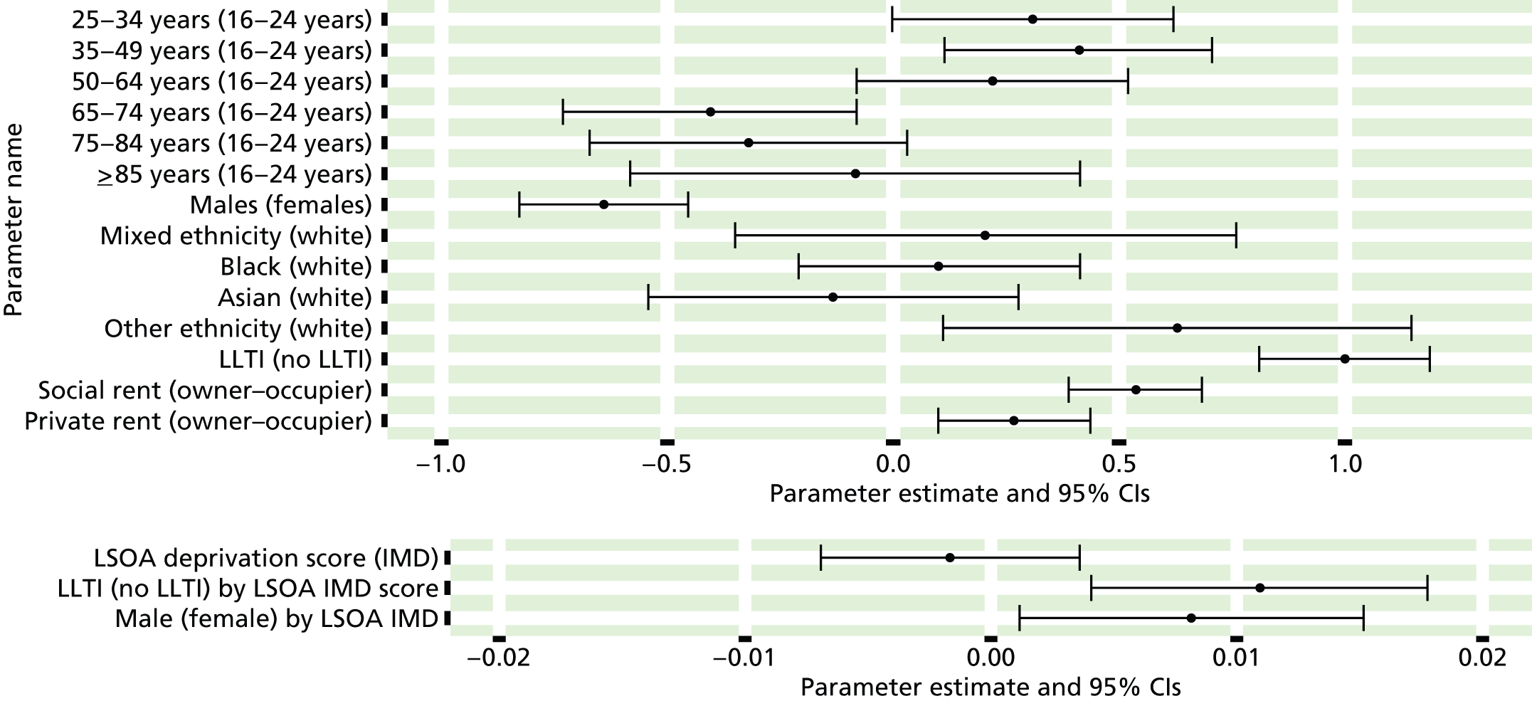
FIGURE 143.
‘Possible’ psychiatric morbidity (UKHLS wave 1, GHQ12 score of ≥ 4) or depression/anxiety drugs: individual estimates and their 95% CIs. (a) MSOAs; (b) LAs; (c) CCGs; and (d) regions (GORs).

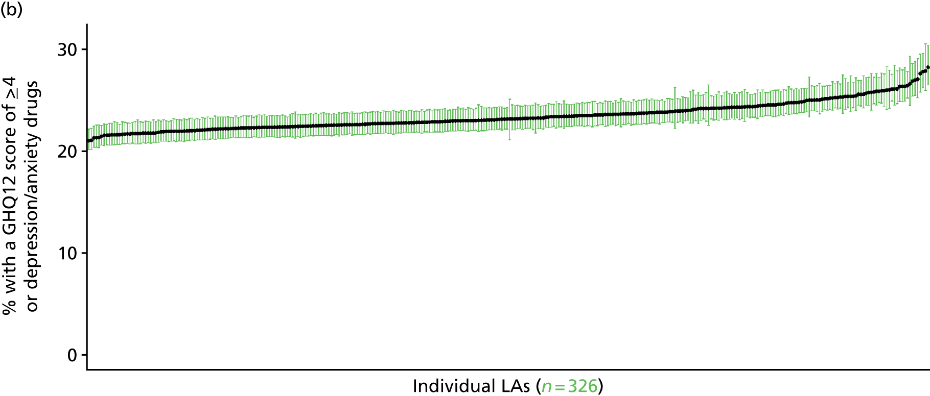

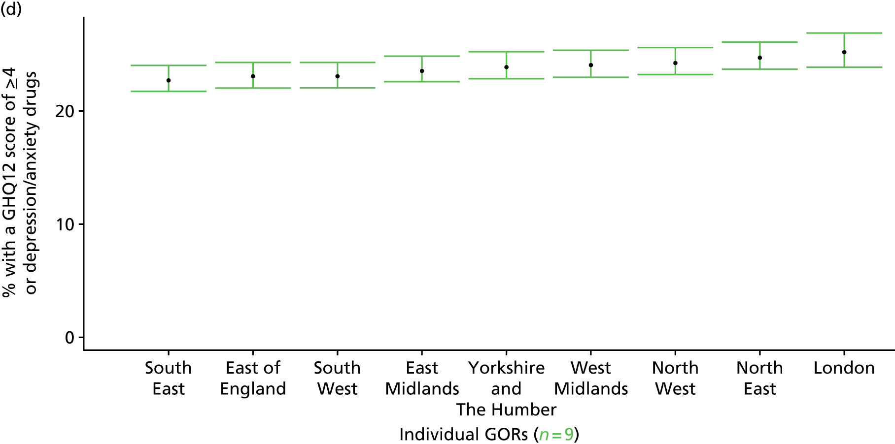
‘Probable’ psychiatric morbidity (12-item General Health Questionnaire score ≥ 6) or currently prescribed depression/anxiety drugs (UK Household Longitudinal Survey, wave 1, 2009–11)
FIGURE 144.
‘Possible’ psychiatric morbidity (UKHLS wave 1, GHQ12 ≥ 6) or depression/anxiety drugs: LSOA-level map. Contains Ordnance Survey data © Crown copyright and database right 2012.
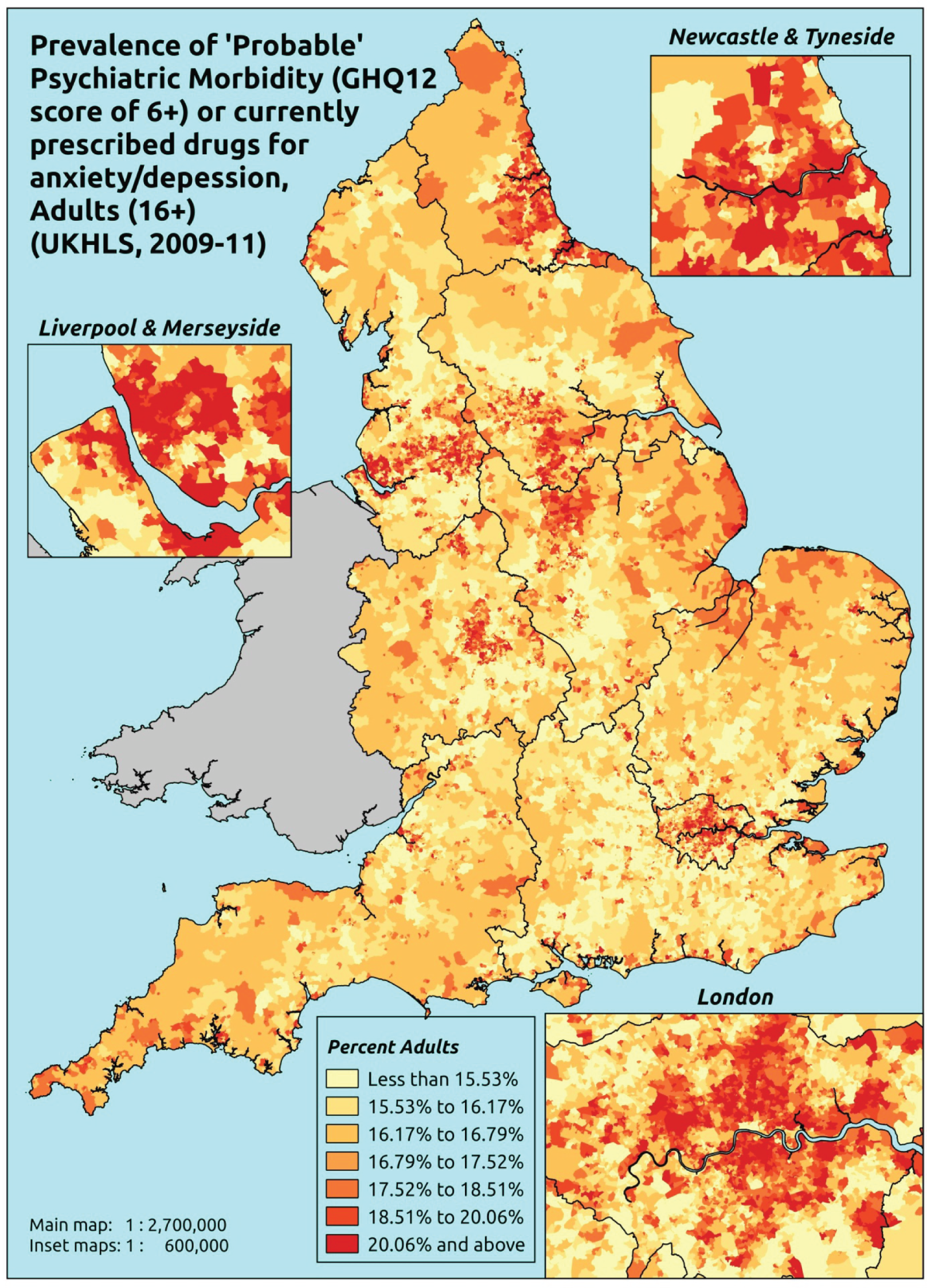
Response variable definition, provenance and prediction
This marker of mental health needs is derived from the 2009–11 first wave of the UKHLS GHQ12 questionnaire score and questions therein about what medicines the respondent is currently being prescribed. This marker captures respondents with a GHQ12 score of ≥ 6 using the standard 0–12 ‘caseness’ scoring approach or who are currently being prescribed drugs for depression and/or anxiety (BNF 4.1.1–4.1.3 or 4.3.1–4.3.4487). In the literature, a score of ≥ 4 is usually taken as being indicative of ‘possible psychiatric morbidity’, but occasionally a ≥ 6 threshold is used. For convenience (and without clinical justification) we describe this as a marker of ‘probable psychiatric morbidity’ – to distinguish this marker from those using the standard ≥ 4 threshold (‘possible psychiatric morbidity’) and the higher ≥ 8 threshold (‘psychiatric morbidity’). We have no information regarding other forms of treatment for mental health issues. This marker recognises the fact that individuals may return a GHQ12 score of < 6 because they are being receiving medication for anxiety/depression and thus aims to capture underlying levels of ‘probable psychiatric morbidity’. This marker is affected by the fact that (a) other types of medication, and other forms of treatment, are not captured, and (b) any sociodemographic and/or geographic variations in access to, or uptake of, prescribing.
The first wave of the UKHLS data set (n = 50,994) runs from January 2009 to January 2011 and includes multiple household respondents aged ≥ 16 years from across the UK. Here the analytical data set is drawn from the subset of respondents living in England and for whom data are available across all model response and predictor variables, namely that they completed the GHQ12 questionnaire and we know what medication they were currently being prescribed, along with information on age band, sex, ethnicity, LLTI, tenure and the IMD score of the LSOA of residence (n = 12,113). A single randomly selected adult is then drawn from each household, resulting in an analytical data set of 8340 adults aged ≥ 16 years.
| Age band (years) | Females | Age band (years) | Males | ||||
|---|---|---|---|---|---|---|---|
| Does not have condition | Has condition | % | Does not have condition | Has condition | % | ||
| 16–24 | 161 | 40 | 19.9 | 16–24 | 94 | 12 | 11.3 |
| 25–34 | 515 | 141 | 21.5 | 25–34 | 346 | 48 | 12.2 |
| 35–49 | 1169 | 409 | 25.9 | 35–49 | 736 | 179 | 19.6 |
| 50–64 | 1035 | 386 | 27.2 | 50–64 | 889 | 182 | 17.0 |
| 65–74 | 517 | 109 | 17.4 | 65–74 | 527 | 70 | 11.7 |
| 75–84 | 284 | 58 | 17.0 | 75–84 | 260 | 43 | 14.2 |
| ≥ 85 | 47 | 21 | 30.9 | ≥ 85 | 53 | 9 | 14.5 |
| Females | 3728 | 1164 | 23.8 | Males | 2905 | 543 | 15.7 |
| Total (males and females) | 6633 | 1707 | 20.5 | ||||
Model parameters are applied to microsimulated LSOA-level census data to produce estimates of the number (and proportion) of people with treated or untreated ‘probable psychiatric morbidity (i.e. who would score ≥ 6 on the GHQ12 or be currently prescribed drugs for depression and/or anxiety) in each age–sex cohort (and overall) in each of the 32,844 English LSOAs. As discussed in the report, bootstrapping is used to derive 95% CIs for the estimates. These LSOA-level prevalence rate estimates (and 95% CIs) are aggregated into a number of higher geographies; namely MSOAs, LAs, CCGs and regions (GORs). Proportionate attribution is used to restructure the prevalence rate estimates to align with 2001 MSOAs, as well as GP practice populations as defined by the 2011 NHS ADS.
Table 167 summarises how expected prevalence rates vary by age, sex and local deprivation (as measured by the 2010 IMD). There are 6569 LSOAs (with 9,226,227 adults) classified as being in the least deprived quintile; 6568 LSOAs (9,525,344 adults) in the second least deprived quintile; 6568 LSOAs (9,658,444 adults) in the third least deprived quintile; 6568 LSOAs (9,650,576 adults) in the fourth least deprived quintile; and 6568 LSOAs (9,535,167 adults) in the most deprived quintile. Note that, as a general rule, variations in prevalence rates reflect variations in the socioeconomic composition of populations in the different types of LSOA rather than variations in deprivation per se.
| Cohort | Least deprived quintile LSOAs | Second least deprived quintile LSOAs | Third least deprived quintile LSOAs | Fourth least deprived quintile LSOAs | Most deprived quintile LSOAs | All England |
|---|---|---|---|---|---|---|
| Female 16–24 | 13.7 (10.5 to 17.1) | 14.0 (10.8 to 17.4) | 14.4 (11.2 to 17.8) | 14.7 (11.6 to 18.3) | 15.7 (12.4 to 19.4) | 14.6 (11.4 to 18.1) |
| Female 25–34 | 17.0 (14.7 to 18.9) | 17.5 (15.2 to 19.4) | 18.0 (15.5 to 20.0) | 18.6 (16.1 to 20.9) | 20.0 (17.2 to 22.6) | 18.4 (16.0 to 20.6) |
| Female 35–49 | 22.5 (21.0 to 24.2) | 23.5 (22.2 to 25.2) | 24.6 (23.2 to 26.5) | 26.3 (24.7 to 28.6) | 29.0 (27.3 to 32.1) | 25.2 (23.6 to 27.2) |
| Female 50–64 | 21.2 (19.7 to 22.9) | 22.6 (21.2 to 24.5) | 24.1 (22.8 to 26.1) | 26.5 (25.2 to 28.9) | 30.6 (29.0 to 33.5) | 24.7 (23.4 to 26.8) |
| Female 65–74 | 16.6 (14.6 to 18.7) | 17.5 (15.3 to 19.7) | 18.4 (16.2 to 20.7) | 19.9 (17.5 to 22.7) | 22.2 (19.5 to 25.5) | 18.7 (16.4 to 21.2) |
| Female ≥ 75 | 21.1 (19.0 to 24.4) | 21.8 (19.6 to 25.3) | 22.6 (20.2 to 26.1) | 23.6 (21.1 to 27.6) | 25.2 (22.5 to 29.6) | 22.7 (20.4 to 26.4) |
| Females | 19.7 (17.8 to 21.8) | 20.5 (18.6 to 22.7) | 21.2 (19.3 to 23.6) | 22.3 (20.2 to 25.1) | 24.4 (22.1 to 27.6) | 21.6 (19.6 to 24.1) |
| Male 16–24 | 7.9 (5.9 to 9.8) | 8.3 (6.2 to 10.1) | 8.7 (6.7 to 10.8) | 9.5 (7.1 to 11.7) | 10.5 (7.8 to 12.9) | 9.1 (6.9 to 11.2) |
| Male 25–34 | 10.0 (8.3 to 11.5) | 10.6 (8.8 to 12.1) | 11.2 (9.3 to 12.8) | 12.1 (10.1 to 14.0) | 13.6 (11.5 to 15.7) | 11.8 (9.9 to 13.6) |
| Male 35–49 | 13.1 (11.7 to 14.4) | 14.0 (12.5 to 15.2) | 15.1 (13.6 to 16.5) | 16.9 (15.3 to 18.4) | 19.8 (17.9 to 21.8) | 15.8 (14.3 to 17.2) |
| Male 50–64 | 12.1 (10.8 to 13.2) | 13.2 (11.9 to 14.4) | 14.5 (13.1 to 15.9) | 16.6 (15.0 to 18.2) | 20.0 (18.0 to 22.1) | 15.1 (13.6 to 16.6) |
| Male 65–74 | 9.3 (7.7 to 10.4) | 9.8 (8.2 to 11.2) | 10.5 (8.8 to 12.0) | 11.7 (9.9 to 13.4) | 13.4 (11.3 to 15.6) | 10.7 (9.0 to 12.3) |
| Male ≥ 75 | 11.5 (9.9 to 13.5) | 12.0 (10.2 to 14.1) | 12.6 (10.8 to 14.7) | 13.5 (11.6 to 15.9) | 14.9 (12.8 to 17.6) | 12.7 (10.9 to 15.0) |
| Males | 11.2 (9.7 to 12.6) | 11.9 (10.3 to 13.3) | 12.7 (11.0 to 14.3) | 14.0 (12.2 to 15.8) | 16.1 (14.0 to 18.3) | 13.2 (11.5 to 14.9) |
| All | 15.6 (14.8 to 16.5) | 16.3 (15.5 to 17.2) | 17.1 (16.2 to 18.1) | 18.3 (17.2 to 19.5) | 20.4 (19.1 to 21.9) | 17.6 (16.5 to 18.6) |
| Factor (reference group) | Model coefficients | 95% CI | ||
|---|---|---|---|---|
| Estimate | SE | 2.5% CI | 97.50% | |
| (Intercept) | –2.02646 | 0.20426 | –2.4268 | –1.62611 |
| Age (16–24 years) | ||||
| 25–34 years | 0.25684 | 0.20563 | –0.14620 | 0.65988 |
| 35–49 years | 0.52770 | 0.19570 | 0.14412 | 0.91128 |
| 50–64 years | 0.24382 | 0.20263 | –0.15335 | 0.64098 |
| 65–74 years | –0.09869 | 0.22677 | –0.54316 | 0.34578 |
| 75–84 years | –0.19998 | 0.27321 | –0.73547 | 0.33551 |
| ≥ 85 years | 0.78613 | 0.38871 | 0.02426 | 1.54800 |
| Sex (females) | ||||
| Males | –0.77559 | 0.10669 | –0.98470 | –0.56648 |
| Ethnicity (white) | ||||
| Mixed | –0.21495 | 0.37821 | –0.95624 | 0.52634 |
| Black | –0.54234 | 0.27662 | –1.08452 | –0.00016 |
| Asian | –0.43700 | 0.29533 | –1.01585 | 0.14185 |
| Other | 0.14660 | 0.38027 | –0.59872 | 0.89192 |
| LLTI (no LTTI) | ||||
| LLTI | 1.00689 | 0.38748 | 0.24743 | 1.76634 |
| Tenure (owner–occupier) | ||||
| Social rent | 0.62302 | 0.07932 | 0.46756 | 0.77848 |
| Private rent or other tenure | 0.34836 | 0.09362 | 0.16486 | 0.53185 |
| LSOA IMD deprivation score | ||||
| IMD score | –0.00134 | 0.00298 | –0.00719 | 0.00450 |
| Interaction effects | ||||
| Male by LSOA IMD | 0.01177 | 0.00387 | 0.00419 | 0.01935 |
| LLTI by LSOA IMD score | 0.00835 | 0.00373 | 0.00104 | 0.01566 |
| Male and mixed | 1.34394 | 0.63493 | 0.09947 | 2.58840 |
| Male and black | 0.63417 | 0.38021 | –0.11103 | 1.37938 |
| Male and Asian | 0.36210 | 0.48889 | –0.59612 | 1.32032 |
| Male and other | 0.88742 | 0.58044 | –0.25024 | 2.02508 |
| 25–34 years and LLTI | 0.04767 | 0.42217 | –0.77979 | 0.87512 |
| 35–49 years and LLTI | 0.18798 | 0.38534 | –0.56728 | 0.94324 |
| 50–64 years and LLTI | 0.27516 | 0.38463 | –0.47872 | 1.02904 |
| 65–74 years and LLTI | –0.15978 | 0.40707 | –0.95764 | 0.63809 |
| 75–84 years and LLTI | –0.08834 | 0.44188 | –0.95443 | 0.77776 |
| ≥ 85 years and LLTI | –0.95379 | 0.57293 | –2.07674 | 0.16915 |
FIGURE 145.
Parameter plots: ‘possible’ psychiatric morbidity (UKHLS wave 1, GHQ12 score of ≥ 6) or depression/anxiety drugs.
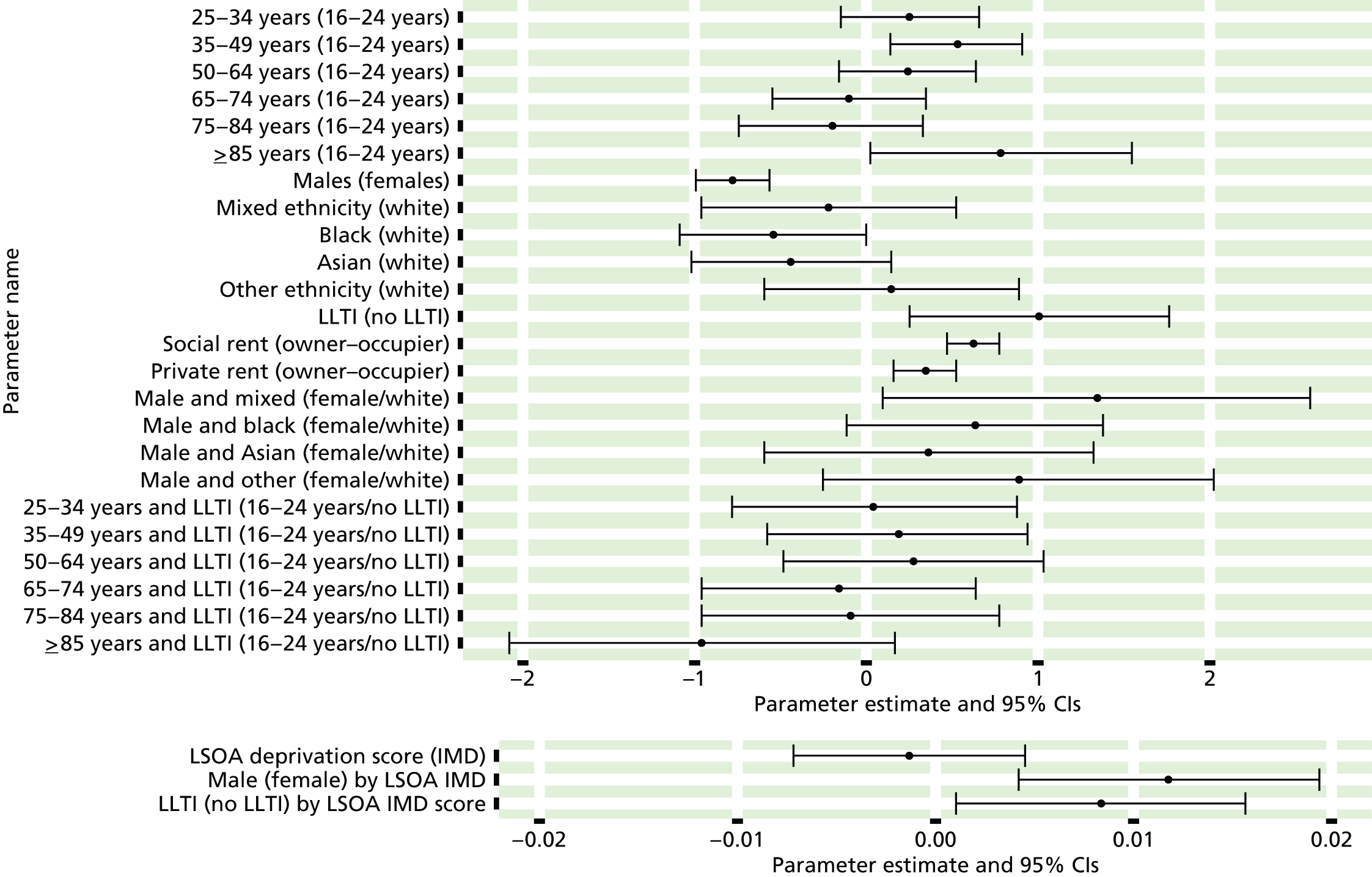
FIGURE 146.
Parameter estimates: ‘possible’ psychiatric morbidity (UKHLS wave 1, GHQ12 score of ≥ 6) or depression/anxiety drugs: individual estimates and their 95% CIs. (a) MSOAs; (b) LAs; (c) CCGs; and (d) regions (GORs).
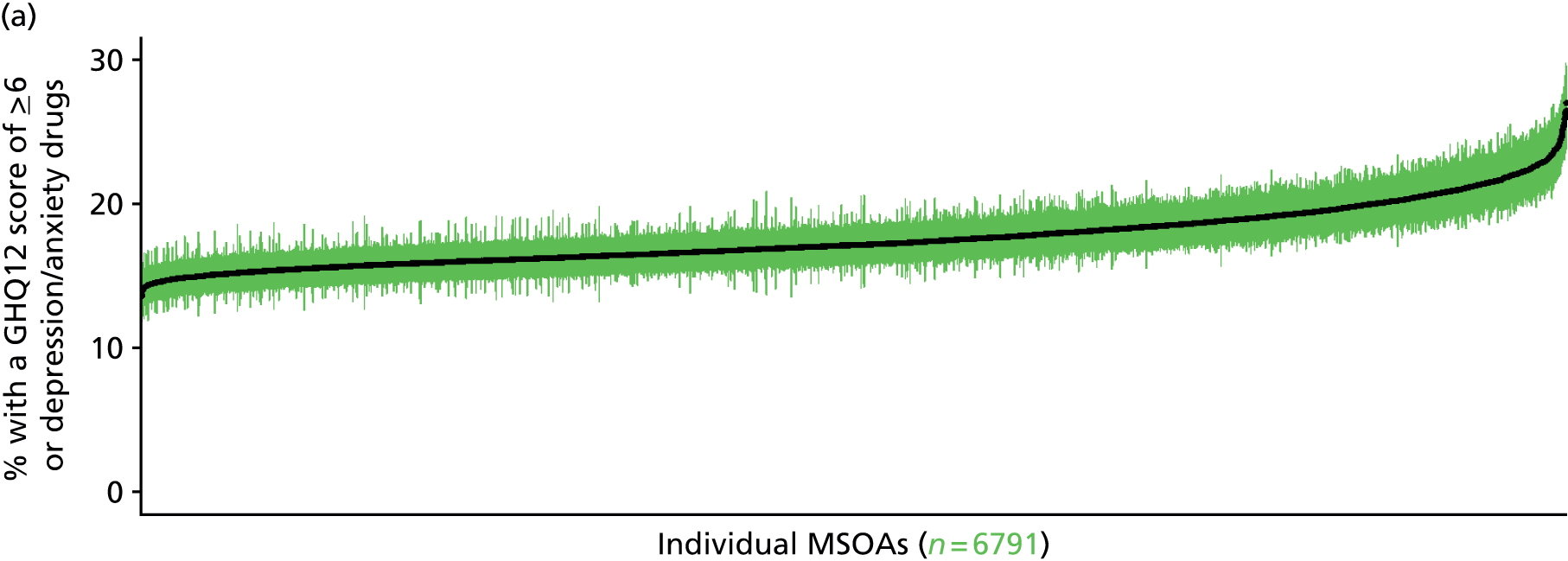
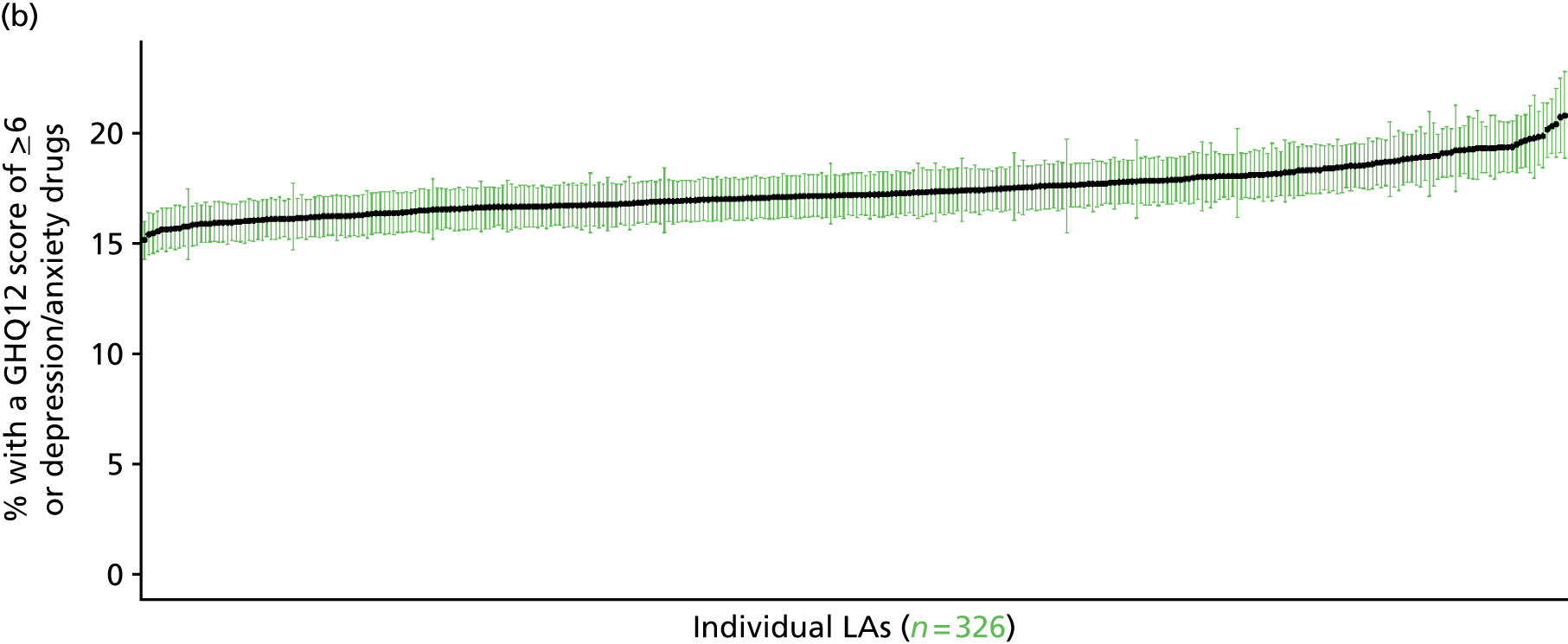

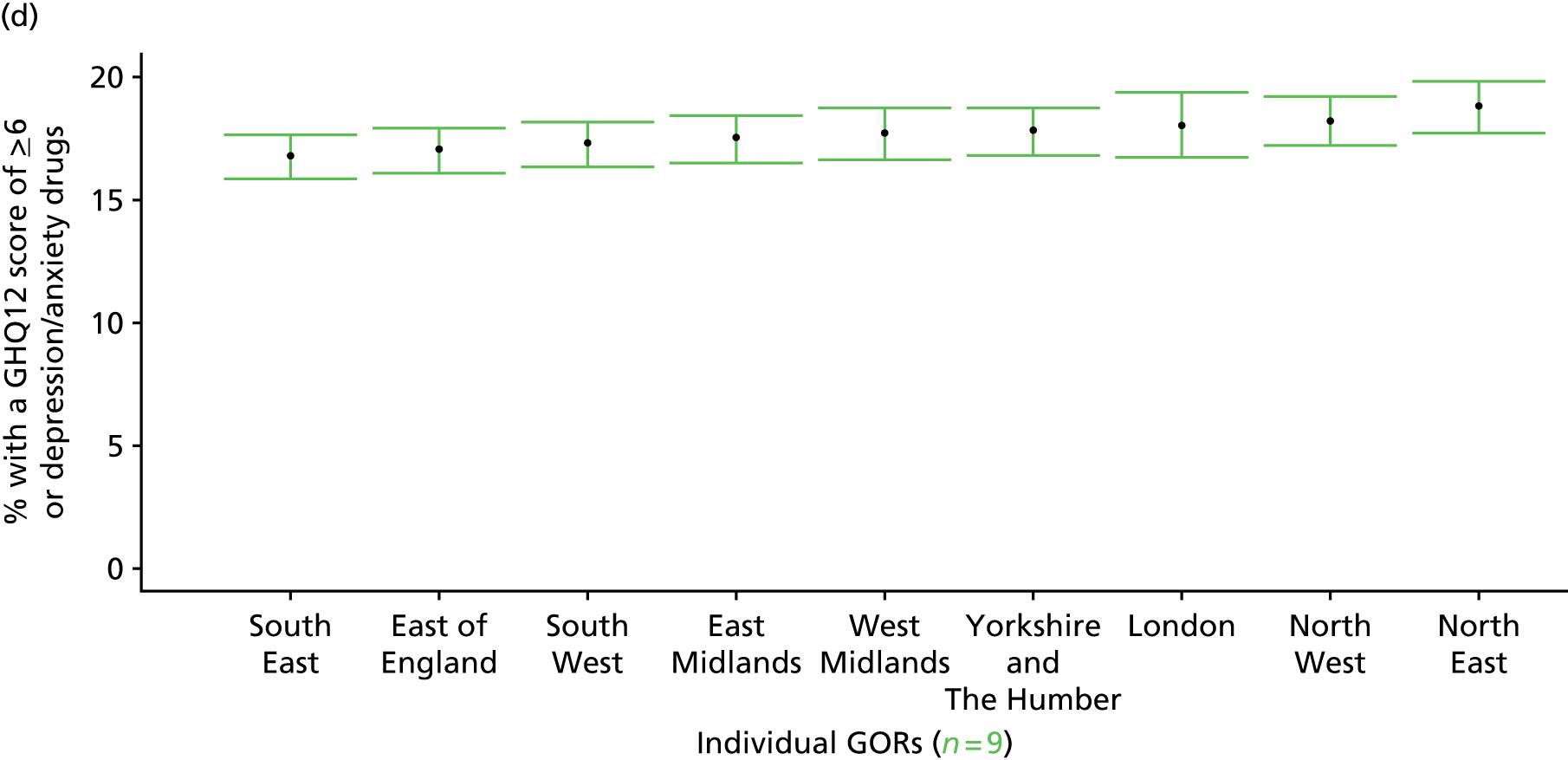
Psychiatric morbidity (12-item General Health Questionnaire score ≥ 8) or currently prescribed depression/anxiety drugs (UK Household Longitudinal Survey, wave 1, 2009–11)
FIGURE 147.
Parameter estimates: ‘possible’ psychiatric morbidity (UKHLS wave 1, GHQ12 score of ≥ 8) or depression/anxiety drugs: LSOA-level map. Contains Ordnance Survey data © Crown copyright and database right 2012.
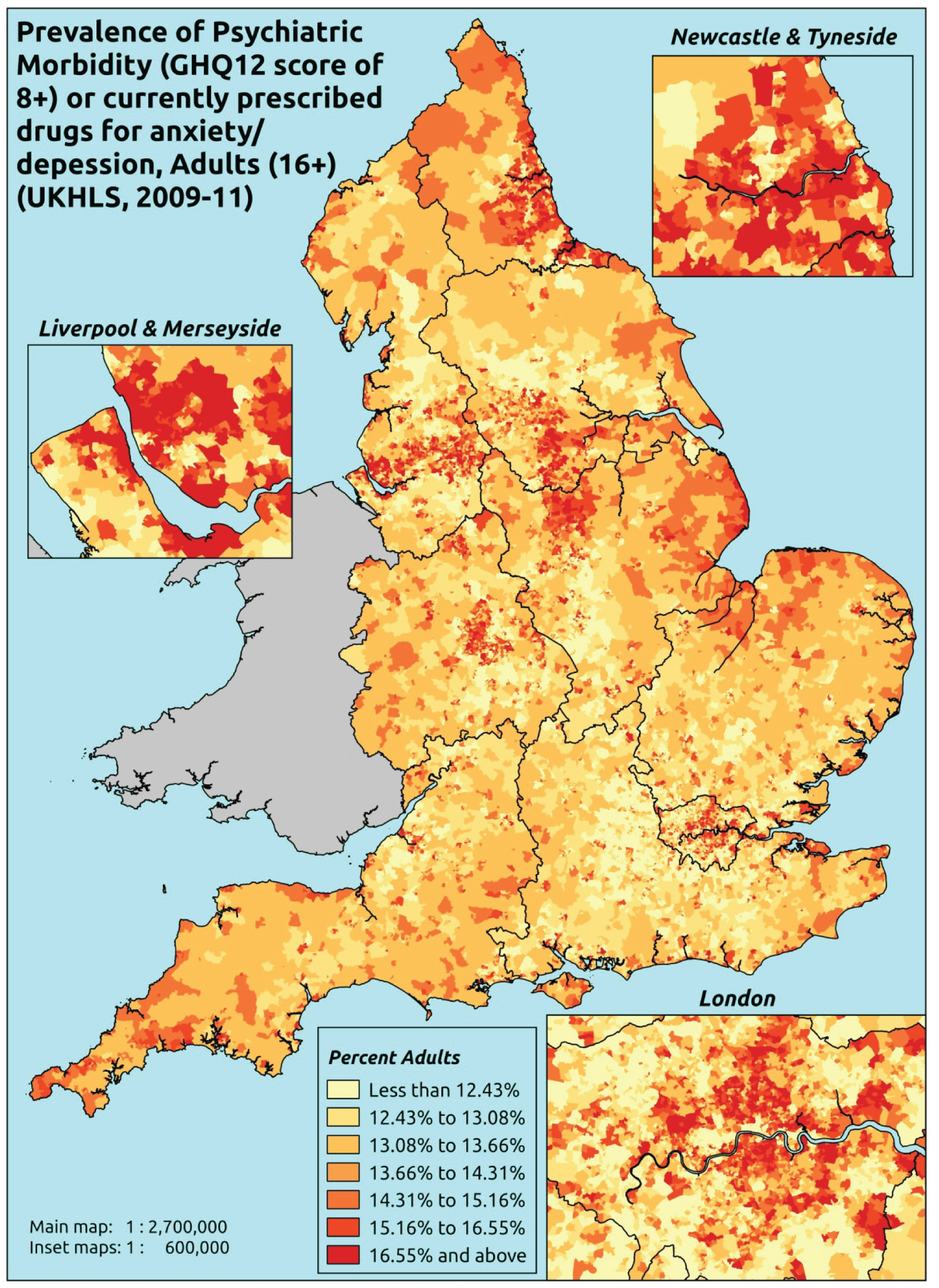
Response variable definition, provenance and prediction
This marker of mental health needs is derived from the 2009–11 first wave of the UKHLS GHQ12 questionnaire score and questions therein about what medicines the respondent is currently being prescribed. This marker captures respondents with a GHQ12 score of ≥ 8 using the standard 0–12 ‘caseness’ scoring approach or who are currently being prescribed drugs for depression and/or anxiety (BNF 4.1.1–4.1.3 or 4.3.1–4.3.4487). In the literature, a score of ≥ 4 is usually taken as being indicative of ‘possible psychiatric morbidity’, but occasionally ≥ 6 or ≥ 8 thresholds are used. For convenience (and without clinical justification) we describe this as a marker of ‘psychiatric morbidity’ – to distinguish it from the standard ≥ 4 threshold (‘possible psychiatric morbidity’) and the ≥ 6 threshold (‘probable psychiatric morbidity’). We have no information regarding other forms of treatment for mental health issues. This marker recognises the fact that individuals may return a GHQ12 score of < 8 because they are being receiving medication for anxiety/depression and thus aims to capture underlying levels of ‘probable psychiatric morbidity’. This marker is affected by the fact that (a) other types of medication, and other forms of treatment, are not captured, and (b) any sociodemographic and/or geographic variations in access to, or uptake of, prescribing.
The first wave of the UKHLS data set (n = 50,994) runs from January 2009 to January 2011 and includes multiple household respondents aged ≥ 16 years from across the UK. Here the analytical data set is drawn from the subset of respondents living in England and for whom data are available across all model response and predictor variables, namely that they completed the GHQ12 questionnaire and we know what medication they were currently being prescribed, along with information on age band, sex, ethnicity, LLTI, tenure and the IMD score of the LSOA of residence (n = 12,113). A single randomly selected adult is then drawn from each household, resulting in an analytical data set of 8340 adults aged ≥ 16 years.
| Age band (years) | Females | Age band (years) | Males | ||||
|---|---|---|---|---|---|---|---|
| Does not have condition | Has condition | % | Does not have condition | Has condition | % | ||
| 16–24 | 172 | 29 | 14.4 | 16–24 | 99 | 7 | 6.6 |
| 25–34 | 537 | 119 | 18.1 | 25–34 | 362 | 32 | 8.1 |
| 35–49 | 1249 | 329 | 20.8 | 35–49 | 761 | 154 | 16.8 |
| 50–64 | 1088 | 333 | 23.4 | 50–64 | 913 | 158 | 14.8 |
| 65–74 | 535 | 91 | 14.5 | 65–74 | 540 | 57 | 9.5 |
| 75–84 | 297 | 45 | 13.2 | 75–84 | 270 | 33 | 10.9 |
| ≥ 85 | 50 | 18 | 26.5 | ≥ 85 | 56 | 6 | 9.7 |
| Females | 3928 | 964 | 19.7 | Males | 3001 | 447 | 13.0 |
| Total (males and females) | 6929 | 1411 | 16.9 | ||||
Model parameters are applied to microsimulated LSOA-level census data to produce estimates of the number (and proportion) of people with treated or untreated ‘psychiatric morbidity (i.e. who would score ≥ 8 on the GHQ12 or be currently prescribed drugs for depression and/or anxiety) in each age–sex cohort (and overall) in each of the 32,844 English LSOAs. As discussed in the report, bootstrapping is used to derive 95% CIs for the estimates. These LSOA-level prevalence rate estimates (and 95% CIs) are aggregated into a number of higher geographies, namely MSOAs, LAs, CCGs and regions (GORs). Proportionate attribution is used to restructure the prevalence rate estimates to align with 2001 MSOAs, as well as GP practice populations as defined by the 2011 NHS ADS.
Table 170 summarises how expected prevalence rates vary by age, sex and local deprivation (as measured by the 2010 IMD). There are 6569 LSOAs (with 9,226,227 adults) classified as being in the least deprived quintile; 6568 LSOAs (9,525,344 adults) in the second least deprived quintile; 6568 LSOAs (9,658,444 adults) in the third least deprived quintile; 6568 LSOAs (9,650,576 adults) in the fourth least deprived quintile; and 6568 LSOAs (9,535,167 adults) in the most deprived quintile. Note that, as a general rule, variations in prevalence rates reflect variations in the socioeconomic composition of populations in the different types of LSOA rather than variations in deprivation per se.
| Cohort | Least deprived quintile LSOAs | Second least deprived quintile LSOAs | Third least deprived quintile LSOAs | Fourth least deprived quintile LSOAs | Most deprived quintile LSOAs | All England |
|---|---|---|---|---|---|---|
| Female 16–24 | 10.6 (7.4 to 13.7) | 10.8 (7.6 to 13.9) | 10.9 (7.8 to 14.1) | 11.2 (8.1 to 14.4) | 12.0 (8.7 to 15.5) | 11.2 (8.0 to 14.3) |
| Female 25–34 | 15.3 (12.8 to 17.1) | 15.5 (13.2 to 17.5) | 15.8 (13.4 to 17.8) | 16.3 (13.9 to 18.6) | 17.6 (15.0 to 20.2) | 16.3 (13.8 to 18.4) |
| Female 35–49 | 17.4 (16.1 to 19.2) | 18.3 (16.9 to 20.3) | 19.3 (18.0 to 21.4) | 20.8 (19.2 to 23.2) | 23.5 (21.6 to 26.0) | 19.8 (18.4 to 22.1) |
| Female 50–64 | 18.6 (17.0 to 20.3) | 19.9 (18.2 to 21.7) | 21.3 (19.6 to 23.3) | 23.7 (21.7 to 25.8) | 27.6 (25.1 to 30.3) | 21.9 (20.2 to 24.0) |
| Female 65–74 | 4.0 (11.7 to 16.6) | 15.1 (12.6 to 17.7) | 16.3 (13.5 to 19.1) | 18.0 (15.2 to 21.2) | 20.8 (17.4 to 24.4) | 16.6 (13.9 to 19.4) |
| Female ≥ 75 | 18.4 (15.0 to 23.3) | 19.3 (15.7 to 24.4) | 20.1 (16.5 to 25.5) | 21.5 (17.6 to 26.9) | 23.0 (19.2 to 28.8) | 20.3 (16.6 to 25.6) |
| Females | 16.5 (14.4 to 18.9) | 17.3 (15.0 to 19.8) | 18.0 (15.7 to 20.7) | 19.0 (16.6 to 21.9) | 21.0 (18.3 to 24.2) | 18.4 (16.1 to 21.1) |
| Male 16–24 | 3.2 (1.3 to 4.9) | 3.3 (1.4 to 5.1) | 3.5 (1.5 to 5.3) | 3.8 (1.6 to 5.8) | 4.3 (1.9 to 6.5) | 3.7 (1.6 to 5.5) |
| Male 25–34 | 5.4 (3.5 to 6.6) | 5.6 (3.7 to 6.9) | 5.9 (3.9 to 7.1) | 6.4 (4.3 to 7.7) | 7.4 (5.1 to 9.0) | 6.3 (4.2 to 7.5) |
| Male 35–49 | 11.4 (9.7 to 12.8) | 12.1 (10.4 to 13.6) | 13.0 (11.3 to 14.6) | 14.6 (12.7 to 16.4) | 17.3 (15.2 to 19.4) | 13.7 (11.9 to 15.4) |
| Male 50–64 | 9.8 (8.3 to 10.9) | 10.7 (9.2 to 11.9) | 11.9 (10.2 to 13.2) | 13.6 (11.9 to 15.3) | 16.6 (14.5 to 18.6) | 12.4 (10.6 to 13.8) |
| Male 65–74 | 7.4 (5.9 to 8.5) | 8.1 (6.5 to 9.3) | 9.0 (7.1 to 10.2) | 10.2 (8.2 to 11.8) | 12.2 (9.7 to 14.2) | 9.2 (7.3 to 10.5) |
| Male ≥ 75 | 10.1 (7.5 to 12.1) | 10.7 (7.9 to 12.8) | 11.4 (8.4 to 13.7) | 12.4 (9.2 to 15.1) | 14.0 (10.3 to 17.1) | 11.5 (8.5 to 13.9) |
| Males | 8.7 (6.9 to 10.1) | 9.2 (7.4 to 10.6) | 9.7 (7.8 to 11.2) | 10.6 (8.5 to 12.4) | 12.3 (9.9 to 14.4) | 10.1 (8.1 to 11.7) |
| All | 12.7 (11.9 to 13.3) | 13.4 (12.5 to 14.1) | 14.0 (13.2 to 14.8) | 15.0 (14.1 to 15.9) | 16.8 (15.7 to 18.0) | 14.4 (13.5 to 15.2) |
| Factor (reference group) | Model coefficients | 95% CI | ||
|---|---|---|---|---|
| Estimate | SE | 2.5% CI | 97.50% | |
| (Intercept) | –2.32349 | 0.23244 | –2.77906 | –1.86791 |
| Age (16–24 years) | ||||
| 25–34 years | 0.43262 | 0.23621 | –0.03036 | 0.89560 |
| 35–49 years | 0.52730 | 0.22360 | 0.08904 | 0.96556 |
| 50–64 years | 0.41619 | 0.22567 | –0.02611 | 0.85850 |
| 65–74 years | –0.20511 | 0.24663 | –0.68851 | 0.27829 |
| 75–84 years | –0.53640 | 0.27287 | –1.07121 | –0.00158 |
| ≥ 85 years | 0.21607 | 0.36138 | –0.49224 | 0.92438 |
| Sex (females) | ||||
| Males | –1.48270 | 0.48362 | –2.43060 | –0.53480 |
| Ethnicity (white) | ||||
| Mixed | –0.38407 | 0.52925 | –1.42140 | 0.65326 |
| Black | –1.31403 | 0.43383 | –2.16434 | –0.46372 |
| Asian | –0.53058 | 0.38739 | –1.28985 | 0.22870 |
| Other | –0.19511 | 0.51859 | –1.21155 | 0.82133 |
| LLTI (no LTTI) | ||||
| LLTI | 1.17185 | 0.11274 | 0.95088 | 1.39282 |
| Tenure (owner–occupier) | ||||
| Social rent | 0.70507 | 0.12428 | 0.46148 | 0.94865 |
| Private rent or other tenure | 0.18902 | 0.13545 | –0.07647 | 0.45450 |
| LSOA IMD deprivation score | ||||
| IMD score | –0.00276 | 0.00343 | –0.00949 | 0.00396 |
| Interaction effects | ||||
| Male by LSOA IMD | 0.01498 | 0.00414 | 0.00686 | 0.02309 |
| LLTI by LSOA IMD score | 0.00788 | 0.00434 | –0.00061 | 0.01638 |
| Male and mixed | 1.47169 | 0.70144 | 0.09687 | 2.84650 |
| Male and black | 0.77491 | 0.48206 | –0.16992 | 1.71975 |
| Male and Asian | 0.07344 | 0.57112 | –1.04596 | 1.19283 |
| Male and other | 1.24587 | 0.68845 | –0.10350 | 2.59523 |
| Mixed and LLTI | –0.09544 | 0.67417 | –1.41682 | 1.22593 |
| Black and LLTI | 1.21832 | 0.47806 | 0.28132 | 2.15532 |
| Asian and LLTI | 0.20579 | 0.54851 | –0.86929 | 1.28088 |
| Other and LLTI | –0.99885 | 0.82038 | –2.60680 | 0.60910 |
| 25–34 years and male | 0.12979 | 0.51222 | –0.87416 | 1.13373 |
| 35–49 years and male | 0.85024 | 0.47842 | –0.08745 | 1.78794 |
| 50–64 years and male | 0.61114 | 0.47886 | –0.32743 | 1.54970 |
| 65–74 years and male | 0.64353 | 0.50164 | –0.33968 | 1.62674 |
| 75–84 years and male | 1.03951 | 0.52902 | 0.00263 | 2.07638 |
| ≥ 85 years and male | 0.10222 | 0.70582 | –1.28119 | 1.48562 |
| LLTI and social rent | –0.06301 | 0.16695 | –0.39023 | 0.26421 |
| LLTI and private rent or other tenure | 0.40662 | 0.20320 | 0.00835 | 0.80488 |
FIGURE 148.
Parameter plots: ‘possible’ psychiatric morbidity (UKHLS wave 1, GHQ12 score of ≥ 8) or depression/anxiety drugs.
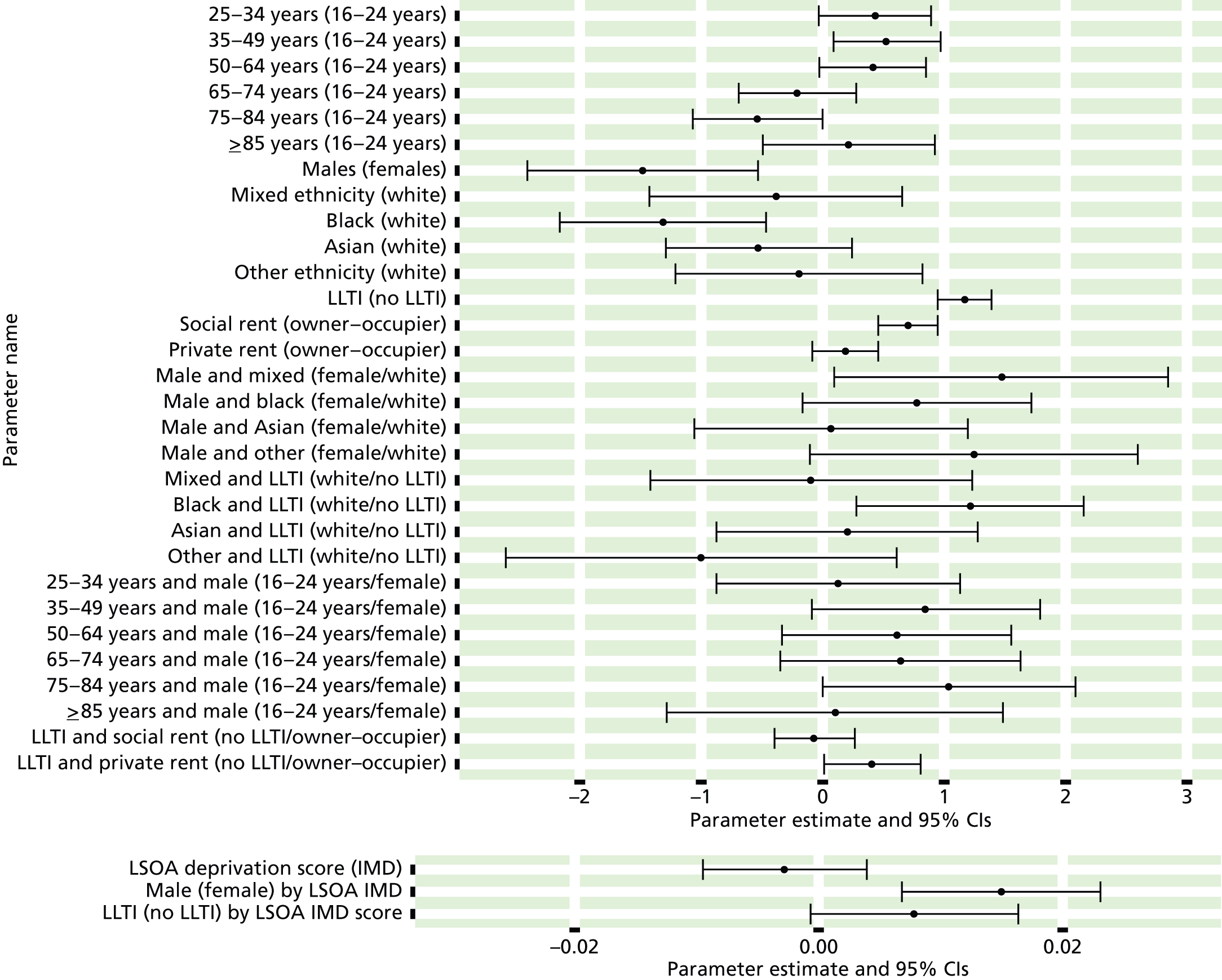
FIGURE 149.
Parameter estimates: ‘possible’ psychiatric morbidity (UKHLS wave 1, GHQ12 score of ≥ 8) or depression/anxiety drugs: individual estimates and their 95% CIs. (a) MSOAs; (b) LAs; (c) CCGs; and (d) regions (GORs).
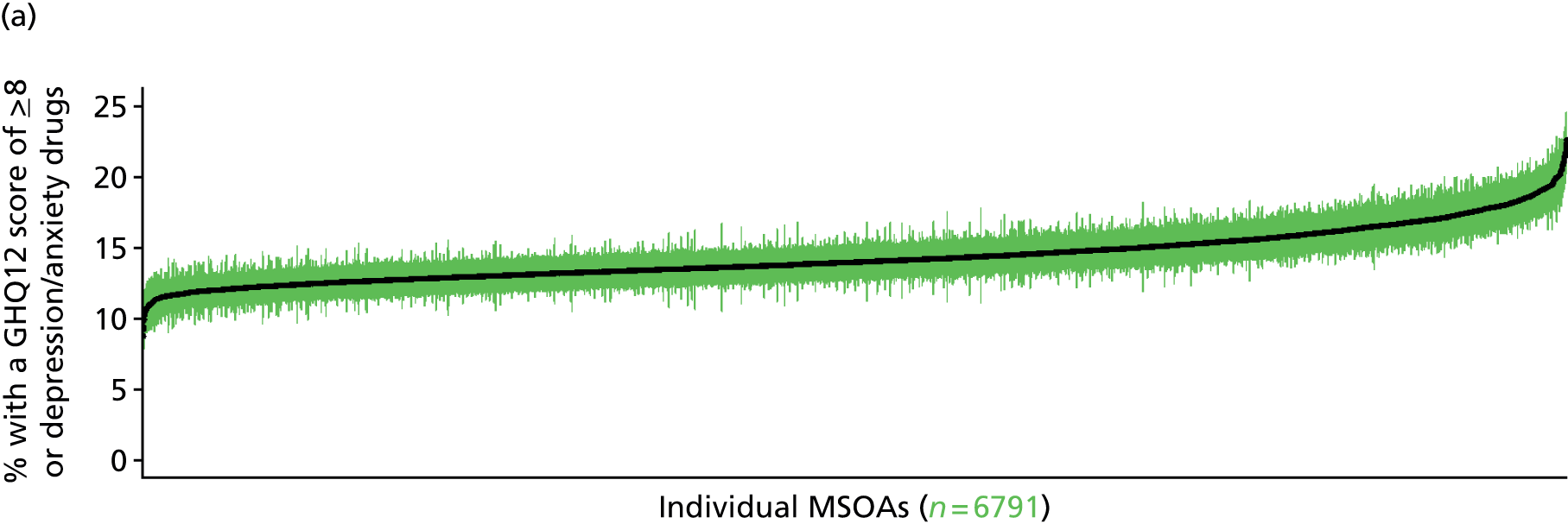
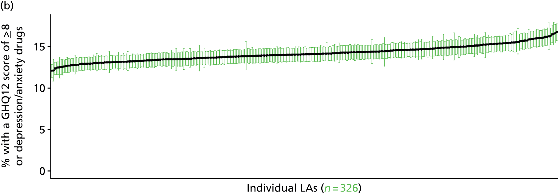


‘Possible’ psychiatric morbidity (12-item General Health Questionnaire score of ≥ 4) (UK Household Longitudinal Survey wave 2, 2010–12)
FIGURE 150.
‘Possible’ psychiatric morbidity (UKHLS wave 2, GHQ12 score of ≥ 4): LSOA-level map. Contains Ordnance Survey data © Crown copyright and database right 2012.
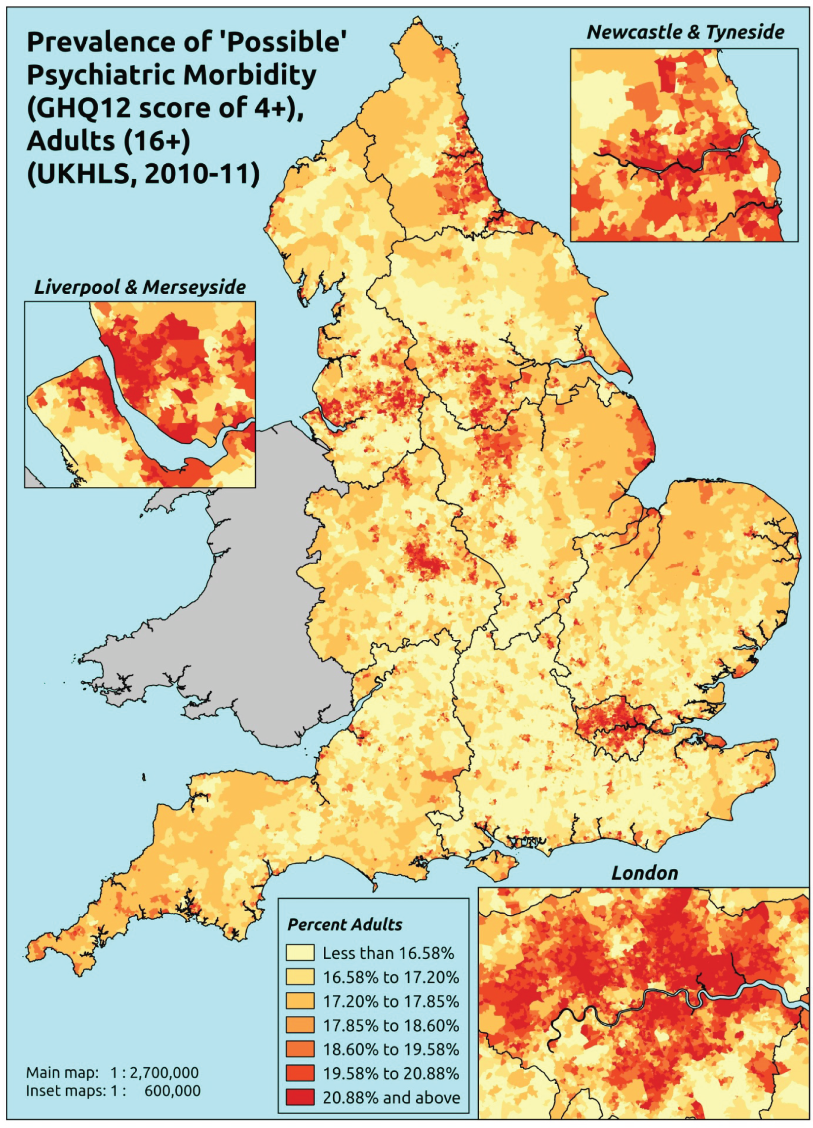
Response variable definition, provenance and prediction
Based on the GHQ12 incorporated within the 2010–12 second wave of the UKHLS, here we capture whether respondents score ≥ 4 more using the standard 0–12 ‘caseness’ scoring approach. The GHQ12 is a screening device for identifying minor psychiatric disorders in the general population. It assesses the respondent’s current state and asks if that differs from their usual state. It is sensitive to short-term psychiatric disorders but not long-standing attributes of the respondent. In the literature, a score of ≥ 4 is usually taken as being indicative of ‘possible psychiatric morbidity’. This is not independent of sociodemographic or geographic variations in access to, or uptake of, care, as individuals may score ≤ 4 because they are currently being treated for a mental health issue. [See ‘Possible’ psychiatric morbidity (12-item General Health Questionnaire score of ≥ 4) or currently prescribed depression/anxiety drugs (UK Household Longitudinal Survey, 2010–12) for an alternative marker which includes people currently being treated with medication for anxiety/depression.]
The second wave of the UKHLS data set (n = 31,242) runs from January 2010 to January 2012 and includes multiple household respondents aged ≥ 16 years from across the UK. Here the analytical data set is drawn from the subset of respondents living in England for whom data are available across all model response and predictor variables, namely that they completed the GHQ12, along with information on age band, sex, ethnicity, LLTI, tenure and the IMD score of the LSOA of residence (n = 16,121). A single randomly selected adult is then drawn from each household, resulting in an analytical data set of 10,028 adults aged ≥ 16 years
| Age band (years) | Females | Age band (years) | Males | ||||
|---|---|---|---|---|---|---|---|
| Does not have condition | Has condition | % | Does not have condition | Has condition | % | ||
| 16–24 | 339 | 99 | 22.6 | 16–24 | 291 | 49 | 14.4 |
| 25–34 | 694 | 221 | 24.2 | 25–34 | 476 | 95 | 16.6 |
| 35–49 | 1280 | 372 | 22.5 | 35–49 | 934 | 208 | 18.2 |
| 50–64 | 1156 | 337 | 22.6 | 50–64 | 871 | 171 | 16.4 |
| 65–74 | 624 | 120 | 16.1 | 65–74 | 510 | 90 | 15.0 |
| 75–84 | 411 | 101 | 19.7 | 75–84 | 284 | 48 | 14.5 |
| ≥ 85 | 135 | 25 | 15.6 | ≥ 85 | 62 | 25 | 28.7 |
| Females | 4639 | 1275 | 21.6 | Males | 3428 | 686 | 16.7 |
| Total (males and females) | 8067 | 1961 | 19.6 | ||||
Model parameters are applied to microsimulated LSOA-level census data to produce estimates of the number (and proportion) of people with ‘possible’ psychiatric morbidity (i.e. who would score ≥ 4 on the GHQ12) in each age–sex cohort (and overall) in each of the 32,844 English LSOAs. As discussed in the report, bootstrapping is used to derive 95% CIs for the estimates. These LSOA-level prevalence rate estimates (and 95% CIs) are aggregated into a number of higher geographies, namely MSOAs, LAs, CCGs and regions (GORs). Proportionate attribution is used to restructure the prevalence rate estimates to align with 2001 MSOAs, as well as GP practice populations as defined by the 2011 NHS ADS.
Table 173 summarises how expected prevalence rates vary by age, sex and local deprivation (as measured by the 2010 IMD). There are 6569 LSOAs (with 9,226,227 adults) classified as being in the least deprived quintile; 6568 LSOAs (9,525,344 adults) in the second least deprived quintile; 6568 LSOAs (9,658,444 adults) in the third least deprived quintile; 6568 LSOAs (9,650,576 adults) in the fourth least deprived quintile; and 6568 LSOAs (9,535,167 adults) in the most deprived quintile. Note that, as a general rule, variations in prevalence rates reflect variations in the socioeconomic composition of populations in the different types of LSOA rather than variations in deprivation per se.
| Cohort | Least deprived quintile LSOAs | Second least deprived quintile LSOAs | Third least deprived quintile LSOAs | Fourth least deprived quintile LSOAs | Most deprived quintile LSOAs | All England |
|---|---|---|---|---|---|---|
| Female 16–24 | 18.6 (15.4 to 21.5) | 18.8 (15.7 to 21.9) | 19.4 (16.1 to 22.4) | 20.0 (16.6 to 23.1) | 20.7 (17.2 to 23.9) | 19.6 (16.3 to 22.7) |
| Female 25–34 | 20.4 (17.9 to 22.3) | 20.6 (18.2 to 22.8) | 21.4 (18.7 to 23.6) | 22.3 (19.4 to 24.6) | 23.6 (20.4 to 25.9) | 21.9 (19.1 to 24.1) |
| Female 35–49 | 19.3 (17.8 to 20.8) | 20.1 (18.6 to 21.6) | 21.2 (19.6 to 22.8) | 22.8 (21.0 to 24.6) | 25.1 (23.1 to 27.5) | 21.7 (20.1 to 23.4) |
| Female 50–64 | 19.4 (17.8 to 21.2) | 20.5 (19.0 to 22.4) | 21.9 (20.2 to 23.9) | 24.0 (22.2 to 26.3) | 27.2 (25.1 to 29.9) | 22.4 (20.7 to 24.5) |
| Female 65–74 | 15.1 (13.5 to 17.2) | 16.1 (14.4 to 18.3) | 17.2 (15.4 to 19.6) | 18.9 (16.7 to 21.6) | 21.4 (18.7 to 24.5) | 17.5 (15.6 to 19.9) |
| Female ≥ 75 | 18.5 (15.6 to 21.0) | 19.1 (16.1 to 21.7) | 19.5 (16.5 to 22.4) | 20.4 (17.3 to 23.3) | 21.8 (18.4 to 24.8) | 19.8 (16.7 to 22.6) |
| Females | 18.7 (16.7 to 20.7) | 19.4 (17.4 to 21.5) | 20.5 (18.3 to 22.7) | 21.9 (19.5 to 24.3) | 23.8 (21.1 to 26.5) | 20.9 (18.6 to 23.1) |
| Male 16–24 | 12.1 (9.4 to 14.8) | 12.4 (9.6 to 15.2) | 12.7 (9.9 to 15.7) | 13.2 (10.2 to 16.4) | 13.9 (10.6 to 17.4) | 13.0 (10.0 to 16.0) |
| Male 25–34 | 13.8 (11.3 to 16.2) | 14.3 (11.6 to 16.6) | 14.7 (12.0 to 17.2) | 15.4 (12.8 to 18.1) | 16.7 (13.9 to 19.6) | 15.2 (12.6 to 17.8) |
| Male 35–49 | 14.7 (12.9 to 16.3) | 15.4 (13.6 to 17.1) | 16.5 (14.7 to 18.2) | 18.2 (16.0 to 19.8) | 20.6 (18.3 to 22.7) | 17.1 (15.2 to 18.7) |
| Male 50–64 | 13.5 (11.6 to 15.4) | 14.6 (12.7 to 16.4) | 15.9 (13.8 to 17.9) | 17.8 (15.6 to 20.1) | 20.8 (18.4 to 23.5) | 16.3 (14.2 to 18.4) |
| Male 65–74 | 14.2 (11.9 to 16.5) | 15.3 (12.9 to 18.0) | 16.6 (13.8 to 19.5) | 18.4 (15.3 to 21.8) | 21.0 (17.7 to 24.9) | 16.8 (14.0 to 19.8) |
| Male ≥ 75 | 18.9 (15.9 to 22.6) | 19.5 (16.5 to 23.4) | 20.1 (17.1 to 24.2) | 21.2 (18.1 to 25.5) | 22.4 (19.0 to 26.9) | 20.2 (17.2 to 24.3) |
| Males | 14.4 (12.2 to 16.6) | 15.1 (12.9 to 17.4) | 16.0 (13.6 to 18.4) | 17.1 (14.6 to 19.7) | 18.9 (16.2 to 21.9) | 16.3 (13.9 to 18.8) |
| All | 16.6 (15.8 to 17.3) | 17.4 (16.5 to 18.1) | 18.3 (17.3 to 19.1) | 19.6 (18.4 to 20.5) | 21.4 (20.0 to 22.6) | 18.7 (17.6 to 19.5) |
| Factor (reference group) | Model coefficients | 95% CI | ||
|---|---|---|---|---|
| Estimate | SE | 2.5% CI | 97.50% | |
| (Intercept) | –1.62204 | 0.12941 | –1.87568 | –1.36840 |
| Age (16–24 years) | ||||
| 25–34 years | 0.04183 | 0.14487 | –0.24211 | 0.32578 |
| 35–49 years | –0.09785 | 0.13809 | –0.36850 | 0.17281 |
| 50–64 years | –0.25096 | 0.14557 | –0.53627 | 0.03435 |
| 65–74 years | –0.87799 | 0.18807 | –1.24660 | –0.50938 |
| 75–84 years | –0.58172 | 0.21879 | –1.01054 | –0.15290 |
| ≥ 85 years | –1.60654 | 0.47877 | –2.54493 | –0.66815 |
| Sex (females) | ||||
| Males | –0.53000 | 0.19379 | –0.90983 | –0.15017 |
| Ethnicity (white) | ||||
| Mixed | –0.39650 | 0.29250 | –0.96981 | 0.17681 |
| Black | 0.20093 | 0.14697 | –0.08712 | 0.48899 |
| Asian | 0.20478 | 0.20089 | –0.18896 | 0.59852 |
| Other | 0.31721 | 0.26167 | –0.19566 | 0.83009 |
| LLTI (no LTTI) | ||||
| LLTI | 0.35408 | 0.31407 | –0.26149 | 0.96966 |
| Tenure (owner–occupier) | ||||
| Social rent | 0.29678 | 0.07313 | 0.15344 | 0.44013 |
| Private rent or other tenure | 0.23901 | 0.07976 | 0.08268 | 0.39534 |
| LSOA IMD deprivation score | ||||
| IMD score | 0.00755 | 0.00181 | 0.00399 | 0.01111 |
| Interaction effects | ||||
| Male and LLTI | 0.24955 | 0.12302 | 0.00842 | 0.49068 |
| 25–34 years and male | 0.03373 | 0.23808 | –0.43291 | 0.50037 |
| 35–49 years and male | 0.17236 | 0.21907 | –0.25701 | 0.60173 |
| 50–64 years and male | 0.02002 | 0.22618 | –0.42329 | 0.46334 |
| 65–74 years and male | 0.31722 | 0.25754 | –0.18757 | 0.82201 |
| 75–84 years and male | 0.00523 | 0.28521 | –0.55378 | 0.56425 |
| ≥ 85 years and male | 1.24325 | 0.40095 | 0.45740 | 2.02911 |
| 25–34 years and LLTI | 0.52461 | 0.35818 | –0.17742 | 1.22665 |
| 35–49 years and LLTI | 0.75304 | 0.32928 | 0.10765 | 1.39843 |
| 50–64 years and LLTI | 0.80665 | 0.32771 | 0.16434 | 1.44896 |
| 65–74 years and LLTI | 0.93682 | 0.34947 | 0.25186 | 1.62177 |
| 75–84 years and LLTI | 0.56214 | 0.37066 | –0.16435 | 1.28863 |
| ≥ 85 years and LLTI | 1.31875 | 0.55827 | 0.22453 | 2.41297 |
FIGURE 151.
Parameter plots: ‘possible’ psychiatric morbidity (UKHLS wave 2, GHQ12 score of ≥ 4).
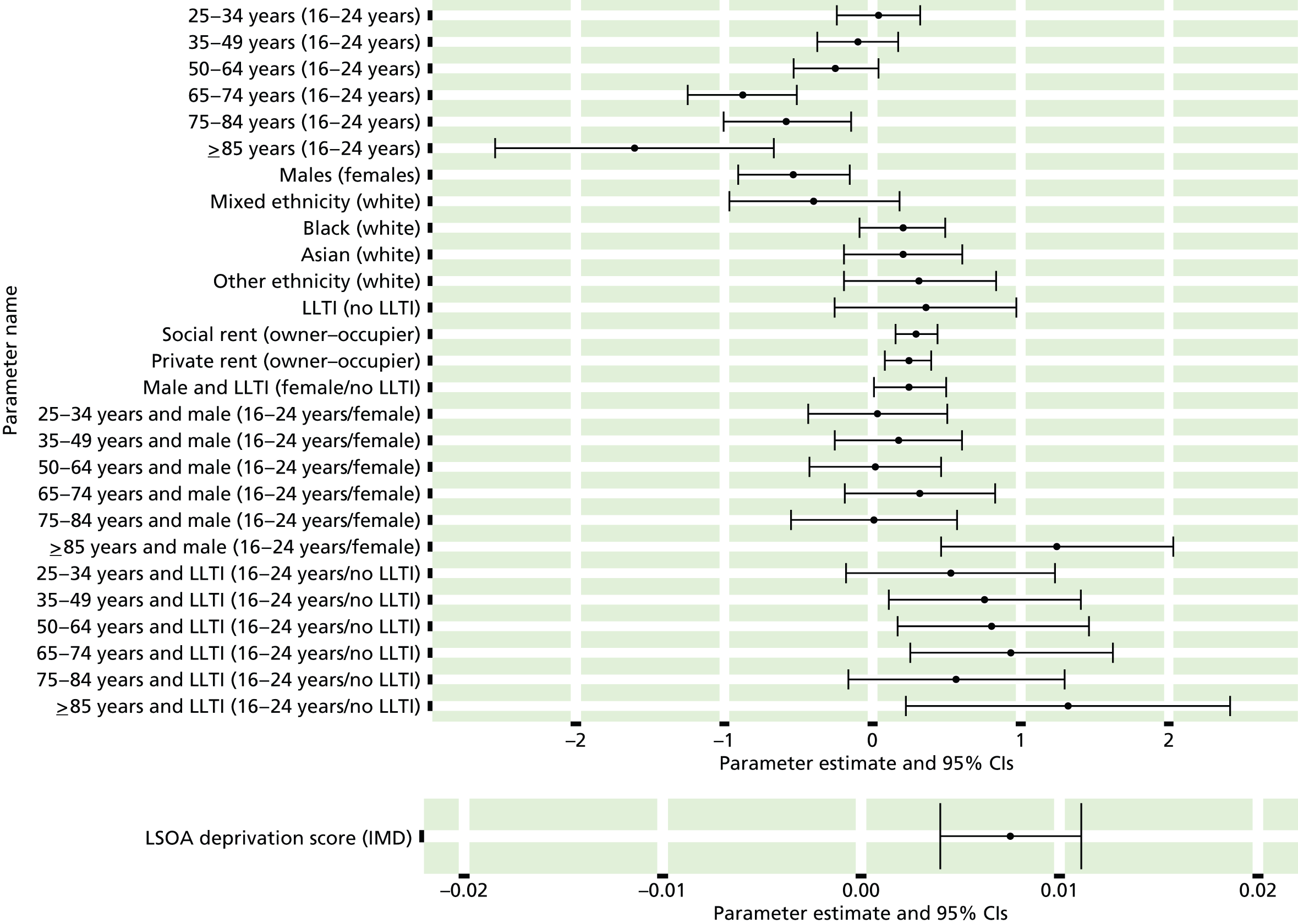
FIGURE 152.
‘Possible’ psychiatric morbidity (UKHLS wave 2, GHQ12 score of ≥ 4): individual estimates and their 95% CIs. (a) MSOAs; (b) LAs; (c) CCGs; and (d) regions (GORs).
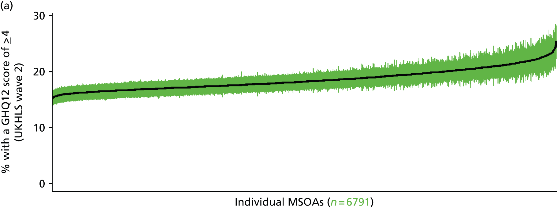
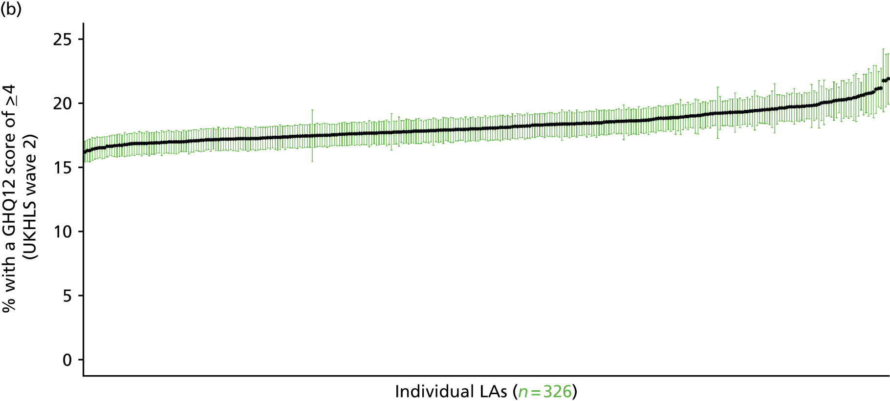
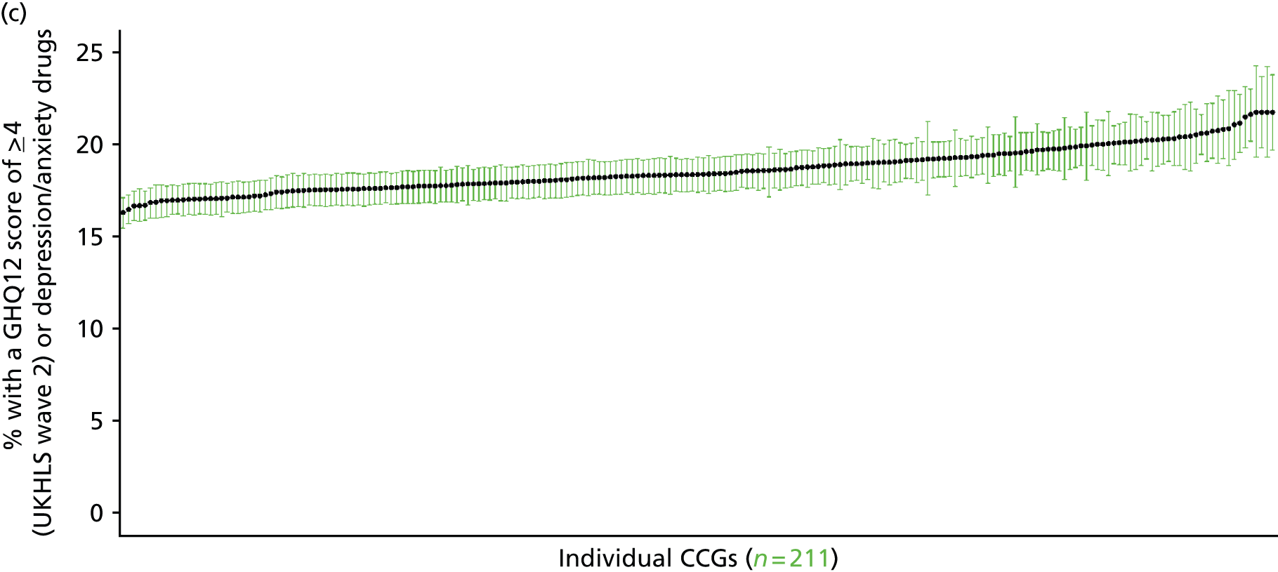
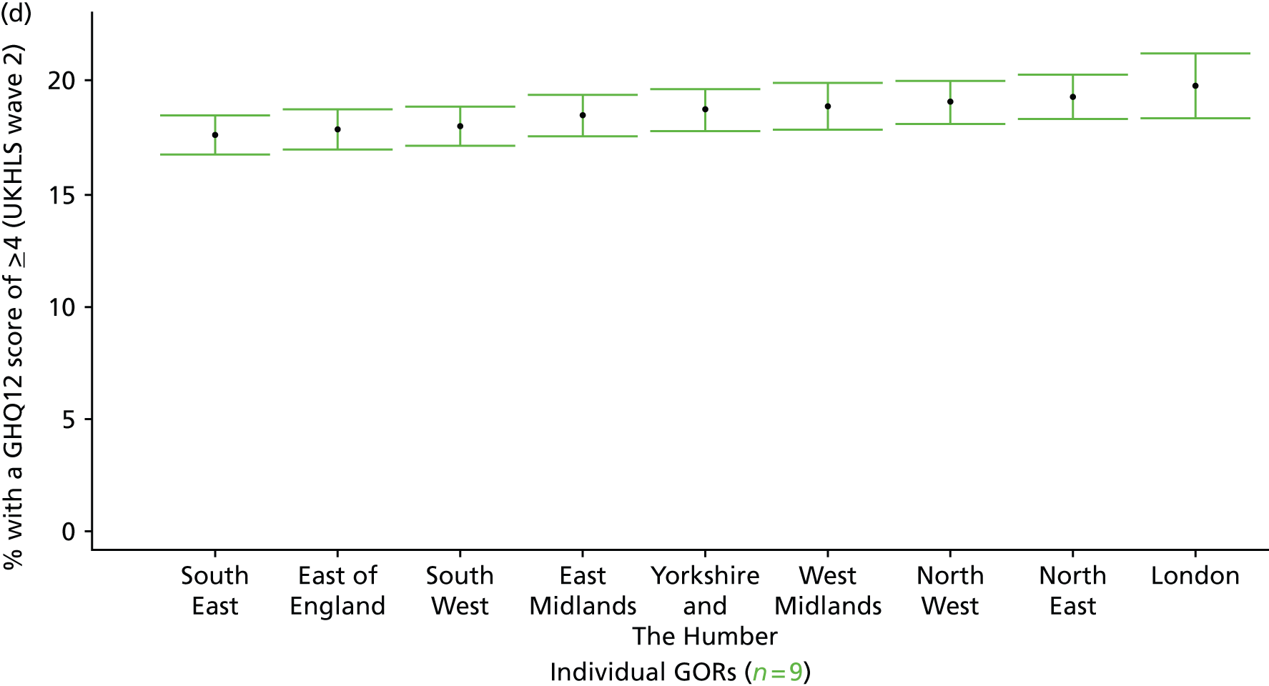
‘Probable’ psychiatric morbidity (12-item General Health Questionnaire score of ≥ 6) (UK Household Longitudinal Survey wave 2, 2010–12)
FIGURE 153.
‘Probable’ psychiatric morbidity (UKHLS wave 2, GHQ12 score of ≥ 6): LSOA-level map. Contains Ordnance Survey data © Crown copyright and database right 2012.

Response variable definition, provenance and prediction
Based on the GHQ12 incorporated within the 2010–12 second wave of the UKHLS, here we capture whether or not respondents score ≥ 6 using the standard 0–12 ‘caseness’ scoring approach. The GHQ12 is a screening device for identifying minor psychiatric disorders in the general population. It assesses the respondent’s current state and asks if that differs from his or her usual state. It is sensitive to short-term psychiatric disorders but not to long-standing attributes of the respondent. In the literature, a score of ≥ 4 is usually taken as being indicative of ‘possible psychiatric morbidity’, but occasionally a ≥ 6 threshold is used. For convenience (and without clinical justification) we describe this as a marker of ‘probable psychiatric morbidity’ to distinguish this marker from those using the standard ≥ 4 threshold (‘possible psychiatric morbidity’) and the higher ≥ 8 threshold (‘psychiatric morbidity’). This is not independent of sociodemographic or geographic variations in access to, or uptake of, care as individuals may score < 6 because they are currently being treated for a mental health issue. (See below for an alternative marker which includes people currently being treated with medication for anxiety/depression.)
The second wave of the UKHLS data set (n = 31,242) runs from January 2010 to January 2012 and includes multiple household respondents aged ≥ 16 years from across the UK. Here the analytical data set is drawn from the subset of respondents living in England for whom data are available across all model response and predictor variables, namely that they completed the GHQ12 questionnaire, along with information on age band, sex, ethnicity, LLTI, tenure and the IMD score of the LSOA of residence (n = 16,121). A single randomly selected adult is then drawn from each household, resulting in an analytical data set of 10,028 adults aged ≥ 16 years.
| Age band (years) | Females | Age band (years) | Males | ||||
|---|---|---|---|---|---|---|---|
| Does not have condition | Has condition | % | Does not have condition | Has condition | % | ||
| 16–24 | 376 | 62 | 14.2 | 16–24 | 310 | 30 | 8.8 |
| 25–34 | 764 | 151 | 16.5 | 25–34 | 505 | 66 | 11.6 |
| 35–49 | 1392 | 260 | 15.7 | 35–49 | 1005 | 137 | 12.0 |
| 50–64 | 1264 | 229 | 15.3 | 50–64 | 928 | 114 | 10.9 |
| 65–74 | 664 | 80 | 10.8 | 65–74 | 536 | 64 | 10.7 |
| 75–84 | 449 | 63 | 12.3 | 75–84 | 292 | 40 | 12.0 |
| ≥ 85 | 150 | 10 | 6.3 | ≥ 85 | 67 | 20 | 23.0 |
| Females | 5059 | 855 | 14.5 | Males | 3643 | 471 | 11.4 |
| Total (males and females) | 8702 | 1326 | 13.2 | ||||
Model parameters are applied to microsimulated LSOA-level census data to produce estimates of the number (and proportion) of people with ‘probable psychiatric morbidity (i.e. who would score ≥ 6 on the GHQ12) in each age–sex cohort (and overall) in each of the 32,844 English LSOAs. As discussed in the report, bootstrapping is used to derive 95% CIs for the estimates. These LSOA-level prevalence rate estimates (and 95% CIs) are aggregated into a number of higher geographies; namely MSOAs, LAs, CCGs and regions (GORs). Proportionate attribution is used to restructure the prevalence rate estimates to align with 2001 MSOAs, as well as GP practice populations as defined by the 2011 NHS ADS.
Table 176 summarises how expected prevalence rates vary by age, sex and local deprivation (as measured by the 2010 IMD). There are 6569 LSOAs (with 9,226,227 adults) classified as being in the least deprived quintile; 6568 LSOAs (9,525,344 adults) in the second least deprived quintile; 6568 LSOAs (9,658,444 adults) in the third least deprived quintile; 6568 LSOAs (9,650,576 adults) in the fourth least deprived quintile; and 6568 LSOAs (9,535,167 adults) in the most deprived quintile. Note that, as a general rule, variations in prevalence rates reflect variations in the socioeconomic composition of populations in the different types of LSOA rather than variations in deprivation per se.
| Cohort | Least deprived quintile LSOAs | Second least deprived quintile LSOAs | Third least deprived quintile LSOAs | Fourth least deprived quintile LSOAs | Most deprived quintile LSOAs | All England |
|---|---|---|---|---|---|---|
| Female 16–24 | 10.9 (8.8 to 13.6) | 11.4 (9.1 to 14.0) | 11.8 (9.5 to 14.4) | 12.4 (9.9 to 15.1) | 13.1 (10.6 to 15.9) | 12.0 (9.7 to 14.8) |
| Female 25–34 | 13.2 (11.3 to 14.9) | 13.6 (11.8 to 15.4) | 14.2 (12.4 to 16.1) | 15.0 (13.0 to 17.0) | 16.1 (13.9 to 18.2) | 14.6 (12.7 to 16.5) |
| Female 35–49 | 13.1 (11.7 to 14.5) | 13.7 (12.2 to 15.1) | 14.6 (13.0 to 16.0) | 15.7 (14.2 to 17.4) | 17.3 (15.5 to 19.4) | 14.9 (13.3 to 16.4) |
| Female 50–64 | 12.7 (11.5 to 14.2) | 13.4 (12.1 to 15.0) | 14.4 (12.9 to 16.1) | 15.8 (14.1 to 17.8) | 17.7 (15.8 to 20.1) | 14.6 (13.2 to 16.4) |
| Female 65–74 | 9.5 (8.0 to 11.7) | 10.0 (8.5 to 12.3) | 10.7 (9.0 to 13.3) | 11.6 (9.9 to 14.5) | 12.9 (10.9 to 16.0) | 10.8 (9.2 to 13.4) |
| Female ≥ 75 | 9.8 (7.7 to 11.5) | 10.0 (7.9 to 11.8) | 10.4 (8.2 to 12.2) | 10.9 (8.6 to 12.9) | 11.6 (9.2 to 13.9) | 10.5 (8.3 to 12.4) |
| Females | 11.9 (10.3 to 13.6) | 12.4 (10.7 to 14.2) | 13.1 (11.3 to 15.0) | 14.1 (12.2 to 16.2) | 15.5 (13.4 to 17.9) | 13.4 (11.6 to 15.4) |
| Male 16–24 | 7.2 (4.9 to 9.2) | 7.4 (5.1 to 9.5) | 7.7 (5.4 to 10.1) | 8.3 (5.8 to 10.6) | 9.0 (6.4 to 11.4) | 8.0 (5.6 to 10.3) |
| Male 25–34 | 9.2 (7.1 to 10.8) | 9.5 (7.3 to 11.3) | 10.0 (7.8 to 11.8) | 10.7 (8.3 to 12.6) | 11.9 (9.2 to 14.1) | 10.5 (8.1 to 12.3) |
| Male 35–49 | 8.9 (7.5 to 10.3) | 9.5 (8.0 to 10.9) | 10.4 (8.7 to 11.9) | 11.6 (9.9 to 13.4) | 13.5 (11.5 to 15.6) | 10.8 (9.1 to 12.4) |
| Male 50–64 | 8.3 (7.1 to 9.7) | 9.2 (7.8 to 10.6) | 10.1 (8.6 to 11.8) | 11.5 (9.8 to 13.5) | 13.5 (11.4 to 16.1) | 10.4 (8.8 to 12.2) |
| Male 65–74 | 9.5 (7.8 to 11.9) | 10.4 (8.6 to 12.9) | 11.3 (9.3 to 14.0) | 12.6 (10.4 to 15.7) | 14.4 (11.7 to 17.9) | 11.4 (9.4 to 14.2) |
| Male ≥ 75 | 14.7 (12.1 to 18.2) | 15.1 (12.6 to 19.0) | 15.9 (13.1 to 19.8) | 16.8 (13.8 to 21.0) | 17.9 (14.6 to 22.3) | 15.9 (13.1 to 19.8) |
| Males | 9.3 (7.6 to 11.2) | 9.9 (8.1 to 11.9) | 10.6 (8.6 to 12.7) | 11.5 (9.3 to 13.7) | 12.8 (10.4 to 15.4) | 10.8 (8.8 to 13.0) |
| All | 10.6 (10.0 to 11.3) | 11.2 (10.5 to 11.9) | 11.9 (11.1 to 12.7) | 12.8 (11.9 to 13.8) | 14.2 (13.1 to 15.3) | 12.2 (11.3 to 13.0) |
| Factor (reference group) | Model coefficients | 95% CI | ||
|---|---|---|---|---|
| Estimate | SE | 2.5% CI | 97.50% | |
| (Intercept) | –2.31048 | 0.15843 | –2.62100 | –1.99996 |
| Age (16–24 years) | ||||
| 25–34 years | 0.18348 | 0.16632 | –0.14250 | 0.50946 |
| 35–49 years | 0.14153 | 0.15829 | –0.16872 | 0.45179 |
| 50–64 years | –0.00373 | 0.16322 | –0.32364 | 0.31618 |
| 65–74 years | –0.50903 | 0.19071 | –0.88281 | –0.13524 |
| 75–84 years | –0.51824 | 0.20409 | –0.91826 | –0.11823 |
| ≥ 85 years | –1.39947 | 0.36317 | –2.11130 | –0.68765 |
| Sex (females) | ||||
| Males | –0.56078 | 0.24119 | –1.03351 | –0.08805 |
| Ethnicity (white) | ||||
| Mixed | –0.97899 | 0.43148 | –1.82469 | –0.13329 |
| Black | 0.32123 | 0.16478 | –0.00174 | 0.64420 |
| Asian | 0.22809 | 0.22469 | –0.21230 | 0.66848 |
| Other | 0.09465 | 0.31553 | –0.52380 | 0.71310 |
| LLTI (no LTTI) | ||||
| LLTI | 0.82270 | 0.12606 | 0.57562 | 1.06979 |
| Tenure (owner–occupier) | ||||
| Social rent | 0.46206 | 0.11680 | 0.23314 | 0.69098 |
| Private rent or other tenure | 0.28671 | 0.11230 | 0.06661 | 0.50681 |
| LSOA IMD deprivation score | ||||
| IMD score | 0.00650 | 0.00278 | 0.00106 | 0.01195 |
| Interaction effects | ||||
| Male and LLTI | 0.50131 | 0.13906 | 0.22875 | 0.77387 |
| 25–34 years and male | 0.07146 | 0.29006 | –0.49705 | 0.63998 |
| 35–49 years and male | 0.04286 | 0.26867 | –0.48374 | 0.56946 |
| 50–64 years and male | –0.08238 | 0.27601 | –0.62336 | 0.45860 |
| 65–74 years and male | 0.27769 | 0.30824 | –0.32645 | 0.88184 |
| 75–84 years and male | 0.20775 | 0.33678 | –0.45233 | 0.86783 |
| ≥ 85 years and male | 1.78644 | 0.49427 | 0.81768 | 2.75520 |
| LLTI and social rent | –0.28543 | 0.16449 | –0.60784 | 0.03698 |
| LLTI and private rent or other tenure | 0.28191 | 0.18802 | –0.08661 | 0.65042 |
| LLTI by LSOA IMD score | 0.00873 | 0.00416 | 0.00058 | 0.01688 |
FIGURE 154.
Parameter plots: ‘probable’ psychiatric morbidity (UKHLS wave 2, GHQ12 score of ≥ 6).

FIGURE 155.
‘Probable’ psychiatric morbidity (UKHLS wave 2, GHQ12 score of ≥ 6): individual estimates and their 95% CIs. (a) MSOAs; (b) LAs; (c) CCGs; and (d) regions (GORs).

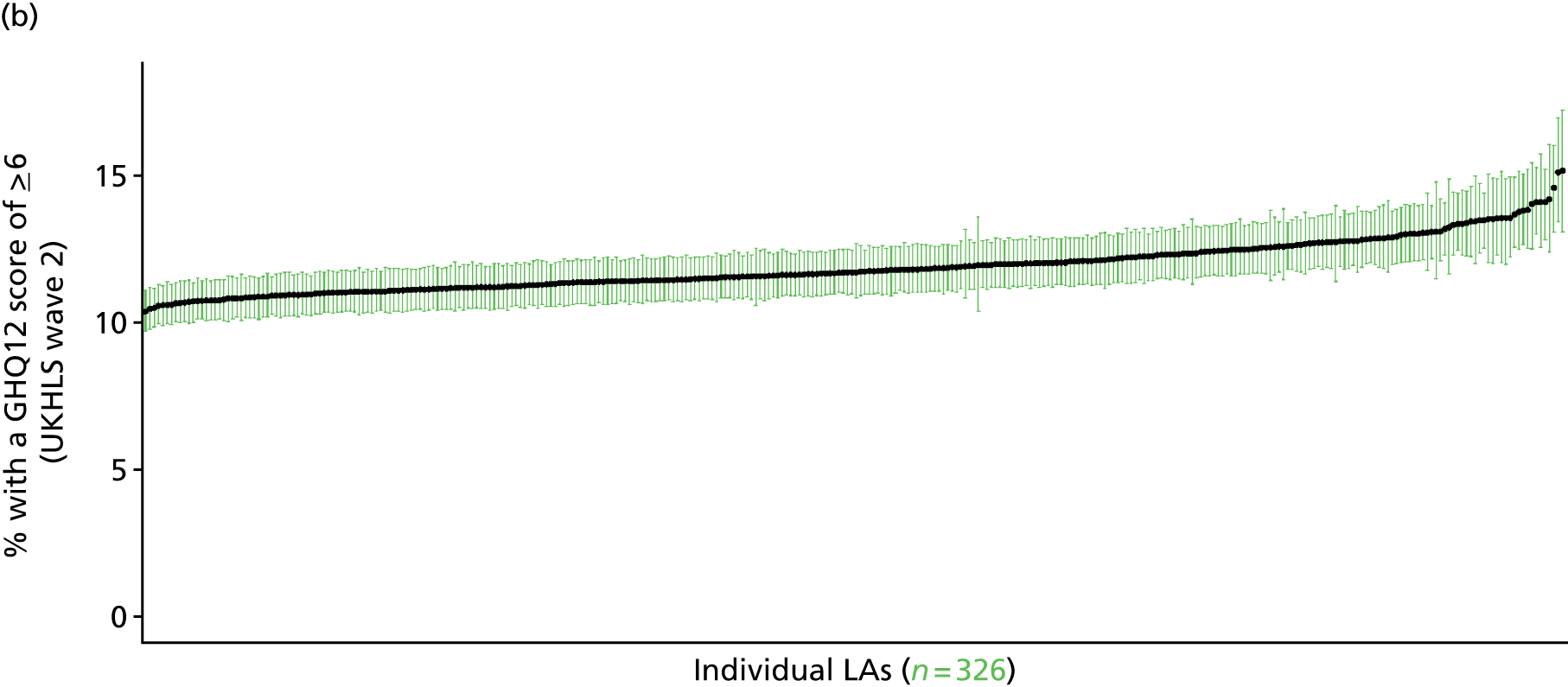

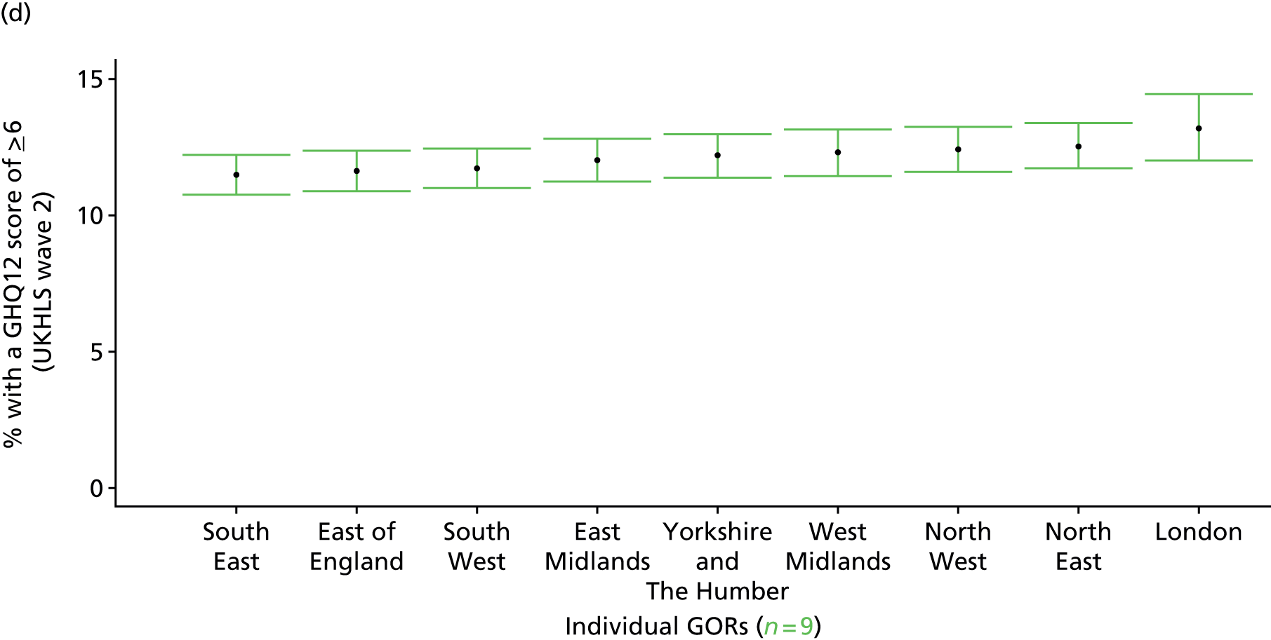
Psychiatric morbidity (12-item General Health Questionnaire score of ≥ 8) (UK Household Longitudinal Survey, wave 2, 2010–12)
FIGURE 156.
Psychiatric morbidity (UKHLS wave 2, GHQ12 score of ≥ 8): LSOA-level map. Contains Ordnance Survey data © Crown copyright and database right 2012.
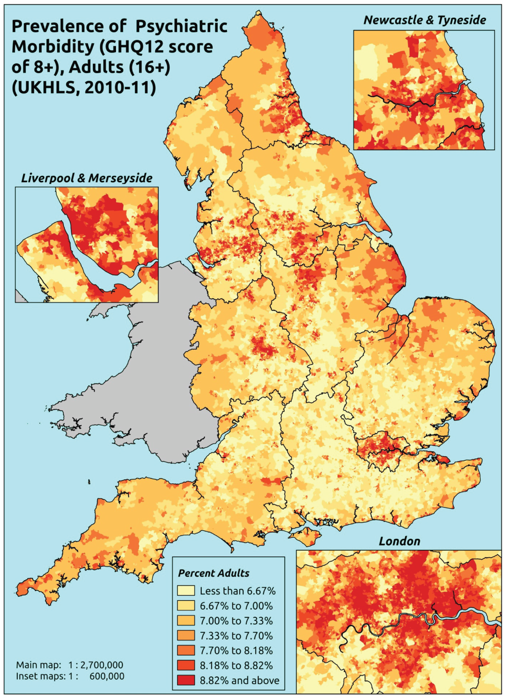
Response variable definition, provenance and prediction
Based on the GHQ12 incorporated within the 2010–12 second wave of the UKHLS, here we capture whether or not respondents score ≥ 8 using the standard 0–12 ‘caseness’ scoring approach. The GHQ12 is a screening device for identifying minor psychiatric disorders in the general population. It assesses the respondent’s current state and asks if that differs from his or her usual state. It is sensitive to short-term psychiatric disorders but not to long-standing attributes of the respondent. In the literature, a score of ≥ 4 is usually taken as being indicative of ‘possible psychiatric morbidity’, but occasionally ≥ 6 or ≥ 8 thresholds are used. For convenience (and without clinical justification) we describe this as a marker of ‘psychiatric morbidity’ – to distinguish it from the standard ≥ 4 threshold (‘possible psychiatric morbidity’) and the ≥ 6 threshold (‘probable psychiatric morbidity’). This is not independent of sociodemographic or geographic variations in access to, or uptake of, care, as individuals may score < 8 because they are currently being treated for a mental health issue. (See below for an alternative marker which includes people currently being treated with medication for anxiety/depression.)
The second wave of the UKHLS data set (n = 31,242) runs from January 2010 to January 2012 and includes multiple household respondents aged ≥ 16 years from across the UK. Here the analytical data set is drawn from the subset of respondents living in England for whom data are available across all model response and predictor variables, namely that they completed the GHQ12, along with information on age band, sex, ethnicity, LLTI, tenure and the IMD score of the LSOA of residence (n = 16,121). A single randomly selected adult is then drawn from each household, resulting in an analytical data set of 10,028 adults aged ≥ 16 years.
| Age band (years) | Females | Age band (years) | Males | ||||
|---|---|---|---|---|---|---|---|
| Does not have condition | Has condition | % | Does not have condition | Has condition | % | ||
| 16–24 | 405 | 33 | 7.5 | 16–24 | 323 | 17 | 5.0 |
| 25–34 | 814 | 101 | 11.0 | 25–34 | 529 | 42 | 7.4 |
| 35–49 | 1491 | 161 | 9.7 | 35–49 | 1054 | 88 | 7.7 |
| 50–64 | 1346 | 147 | 9.8 | 50–64 | 961 | 81 | 7.8 |
| 65–74 | 694 | 50 | 6.7 | 65–74 | 554 | 46 | 7.7 |
| 75–84 | 472 | 40 | 7.8 | 75–84 | 304 | 28 | 8.4 |
| ≥ 85 | 156 | 4 | 2.5 | ≥ 85 | 76 | 11 | 12.6 |
| Females | 5378 | 536 | 9.1 | Males | 3801 | 313 | 7.6 |
| Total (males and females) | 9179 | 849 | 8.5 | ||||
Model parameters are applied to microsimulated LSOA-level census data to produce estimates of the number (and proportion) of people with ‘psychiatric morbidity (i.e. who would score ≥ 8 on the GHQ12) in each age–sex cohort (and overall) in each of the 32,844 English LSOAs. As discussed in the report, bootstrapping is used to derive 95% CIs for the estimates. These LSOA-level prevalence rate estimates (and 95% CIs) are aggregated into a number of higher geographies; namely MSOAs, LAs, CCGs and regions (GORs). Proportionate attribution is used to restructure the prevalence rate estimates to align with 2001 MSOAs, as well as GP practice populations as defined by the 2011 NHS ADS.
Table 179 summarises how expected prevalence rates vary by age, sex and local deprivation (as measured by the 2010 IMD). There are 6569 LSOAs (with 9,226,227 adults) classified as being in the least deprived quintile; 6568 LSOAs (9,525,344 adults) in the second least deprived quintile; 6568 LSOAs (9,658,444 adults) in the third least deprived quintile; 6568 LSOAs (9,650,576 adults) in the fourth least deprived quintile; and 6568 LSOAs (9,535,167 adults) in the most deprived quintile. Note that, as a general rule, variations in prevalence rates reflect variations in the socioeconomic composition of populations in the different types of LSOA rather than variations in deprivation per se.
| Cohort | Least deprived quintile LSOAs | Second least deprived quintile LSOAs | Third least deprived quintile LSOAs | Fourth least deprived quintile LSOAs | Most deprived quintile LSOAs | All England |
|---|---|---|---|---|---|---|
| Female 16–24 | 5.5 (3.8 to 7.4) | 5.7 (4.0 to 7.6) | 5.9 (4.1 to 7.9) | 6.1 (4.3 to 8.2) | 6.5 (4.5 to 8.7) | 6.0 (4.2 to 8.0) |
| Female 25–34 | 8.2 (6.7 to 9.8) | 8.6 (7.0 to 10.1) | 8.8 (7.3 to 10.6) | 9.3 (7.7 to 11.2) | 10.1 (8.3 to 12.1) | 9.1 (7.6 to 11.0) |
| Female 35–49 | 7.7 (6.6 to 8.8) | 8.1 (7.0 to 9.4) | 8.6 (7.6 to 10.1) | 9.5 (8.3 to 11.3) | 10.6 (9.1 to 12.9) | 8.9 (7.8 to 10.5) |
| Female 50–64 | 7.9 (6.8 to 9.0) | 8.5 (7.3 to 9.6) | 9.2 (7.9 to 10.5) | 10.2 (8.8 to 11.6) | 11.7 (10.1 to 13.4) | 9.4 (8.1 to 10.7) |
| Female 65–74 | 6.1 (4.9 to 7.6) | 6.5 (5.2 to 8.1) | 6.9 (5.6 to 8.8) | 7.6 (6.2 to 9.7) | 8.5 (6.8 to 11.1) | 7.0 (5.6 to 8.9) |
| Female ≥ 75 | 6.1 (4.6 to 8.0) | 6.3 (4.7 to 8.2) | 6.5 (4.9 to 8.4) | 6.9 (5.1 to 8.9) | 7.3 (5.4 to 9.5) | 6.6 (4.9 to 8.6) |
| Females | 7.2 (5.9 to 8.6) | 7.6 (6.2 to 9.0) | 8.0 (6.6 to 9.6) | 8.6 (7.1 to 10.5) | 9.5 (7.8 to 11.6) | 8.2 (6.8 to 9.9) |
| Male 16–24 | 3.9 (2.1 to 5.1) | 4.1 (2.2 to 5.2) | 4.3 (2.3 to 5.5) | 4.4 (2.5 to 5.9) | 4.9 (2.7 to 6.4) | 4.4 (2.4 to 5.7) |
| Male 25–34 | 5.5 (4.0 to 6.9) | 5.7 (4.1 to 7.1) | 6.0 (4.3 to 7.4) | 6.4 (4.7 to 7.9) | 7.2 (5.4 to 9.0) | 6.3 (4.6 to 7.7) |
| Male 35–49 | 5.4 (4.5 to 6.5) | 5.9 (4.9 to 7.0) | 6.5 (5.4 to 7.8) | 7.4 (6.1 to 8.8) | 8.7 (7.3 to 10.5) | 6.8 (5.7 to 8.2) |
| Male 50–64 | 5.9 (4.8 to 7.1) | 6.5 (5.4 to 7.9) | 7.3 (6.0 to 8.8) | 8.4 (7.0 to 10.1) | 10.0 (8.3 to 12.2) | 7.5 (6.2 to 9.1) |
| Male 65–74 | 7.1 (5.4 to 8.8) | 7.8 (5.9 to 9.6) | 8.5 (6.5 to 10.4) | 9.5 (7.2 to 11.7) | 10.8 (8.2 to 13.5) | 8.6 (6.5 to 10.5) |
| Male ≥ 75 | 9.9 (7.1 to 12.8) | 10.3 (7.5 to 13.3) | 10.8 (7.9 to 14.0) | 11.4 (8.4 to 14.8) | 12.0 (8.9 to 15.5) | 10.8 (7.8 to 14.0) |
| Males | 6.1 (4.6 to 7.5) | 6.6 (5.0 to 8.1) | 7.0 (5.4 to 8.6) | 7.5 (5.8 to 9.3) | 8.5 (6.5 to 10.5) | 7.1 (5.5 to 8.8) |
| All | 6.7 (6.1 to 7.2) | 7.1 (6.5 to 7.7) | 7.5 (6.9 to 8.2) | 8.1 (7.4 to 8.9) | 9.0 (8.1 to 10.1) | 7.7 (7.0 to 8.4) |
| Factor (reference group) | Model coefficients | 95% CI | ||
|---|---|---|---|---|
| Estimate | SE | 2.5% CI | 97.50% | |
| (Intercept) | –3.10305 | 0.20093 | –3.49687 | –2.70923 |
| Age (16–24 years) | ||||
| 25–34 years | 0.41261 | 0.21262 | –0.00413 | 0.82935 |
| 35–49 years | 0.27287 | 0.20508 | –0.12908 | 0.67483 |
| 50–64 years | 0.15056 | 0.21018 | –0.26140 | 0.56251 |
| 65–74 years | –0.37018 | 0.24336 | –0.84716 | 0.10680 |
| 75–84 years | –0.37897 | 0.25786 | –0.88438 | 0.12644 |
| ≥ 85 years | –1.70579 | 0.54538 | –2.77473 | –0.63685 |
| Sex (females) | ||||
| Males | –0.48237 | 0.31434 | –1.09848 | 0.13374 |
| Ethnicity (white) | ||||
| Mixed | –1.18182 | 0.59449 | –2.34701 | –0.01663 |
| Black | 0.05377 | 0.21289 | –0.36350 | 0.47103 |
| Asian | 0.27567 | 0.26058 | –0.23508 | 0.78641 |
| Other | 0.31980 | 0.35113 | –0.36842 | 1.00802 |
| LLTI (no LTTI) | ||||
| LLTI | 1.10403 | 0.11711 | 0.87449 | 1.33357 |
| Tenure (owner–occupier) | ||||
| Social rent | 0.40696 | 0.13988 | 0.13280 | 0.68113 |
| Private rent or other tenure | 0.20870 | 0.14306 | –0.07170 | 0.48910 |
| LSOA IMD deprivation score | ||||
| IMD score | 0.01097 | 0.00245 | 0.00617 | 0.01577 |
| Interaction effects | ||||
| Male and LLTI | 0.51237 | 0.16464 | 0.18967 | 0.83507 |
| 25–34 years and male | –0.05868 | 0.36932 | –0.78255 | 0.66518 |
| 35–49 years and male | 0.00597 | 0.34526 | –0.67073 | 0.68268 |
| 50–64 years and male | –0.04618 | 0.35139 | –0.73492 | 0.64255 |
| 65–74 years and male | 0.32744 | 0.38781 | –0.43266 | 1.08754 |
| 75–84 years and male | 0.20997 | 0.41914 | –0.61153 | 1.03148 |
| ≥ 85 years and male | 1.84880 | 0.69031 | 0.49578 | 3.20181 |
| LLTI and social rent | –0.33009 | 0.18223 | –0.68725 | 0.02708 |
| LLTI and private rent or other tenure | 0.41548 | 0.21592 | –0.00772 | 0.83867 |
FIGURE 157.
Parameter plots: psychiatric morbidity (UKHLS wave 2, GHQ12 score of ≥ 8).
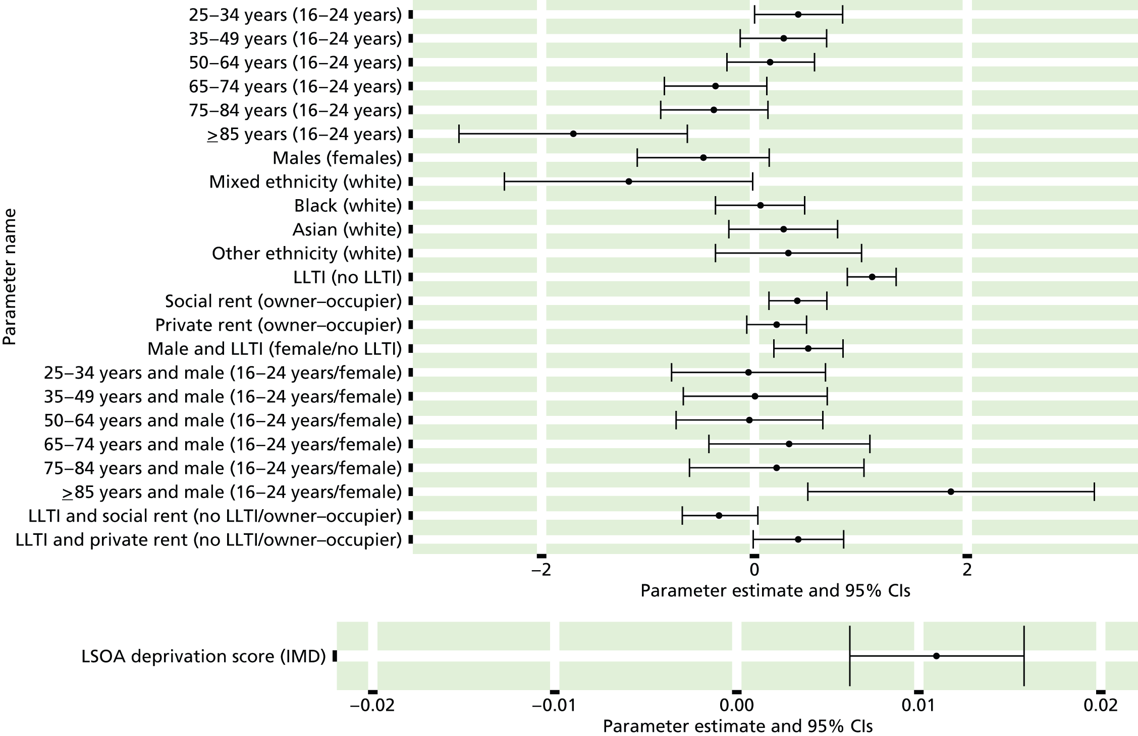
FIGURE 158.
Psychiatric morbidity (UKHLS wave 2, GHQ12 score of ≥ 8): individual estimates and their 95% CIs. (a) MSOAs; (b) LAs; (c) CCGs; and (d) regions (GORs).

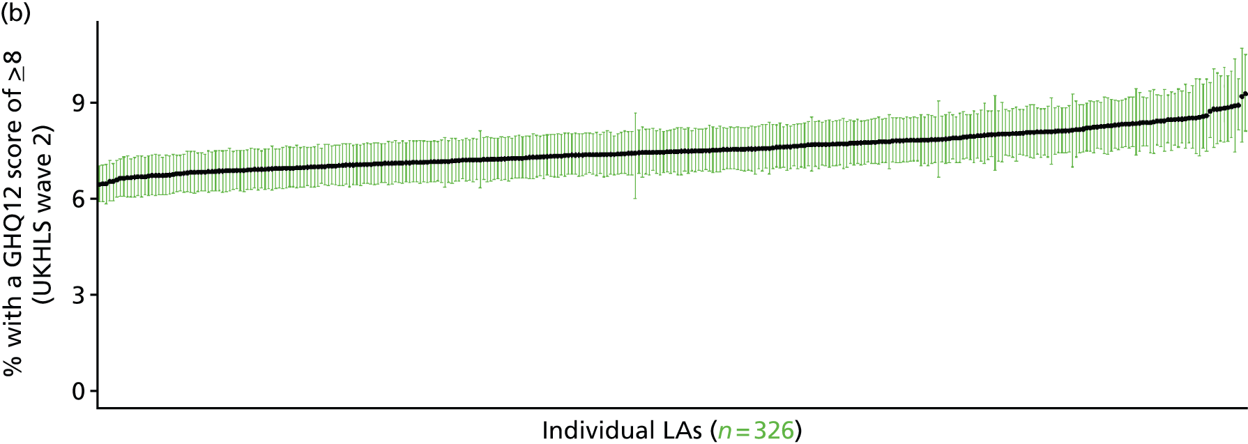
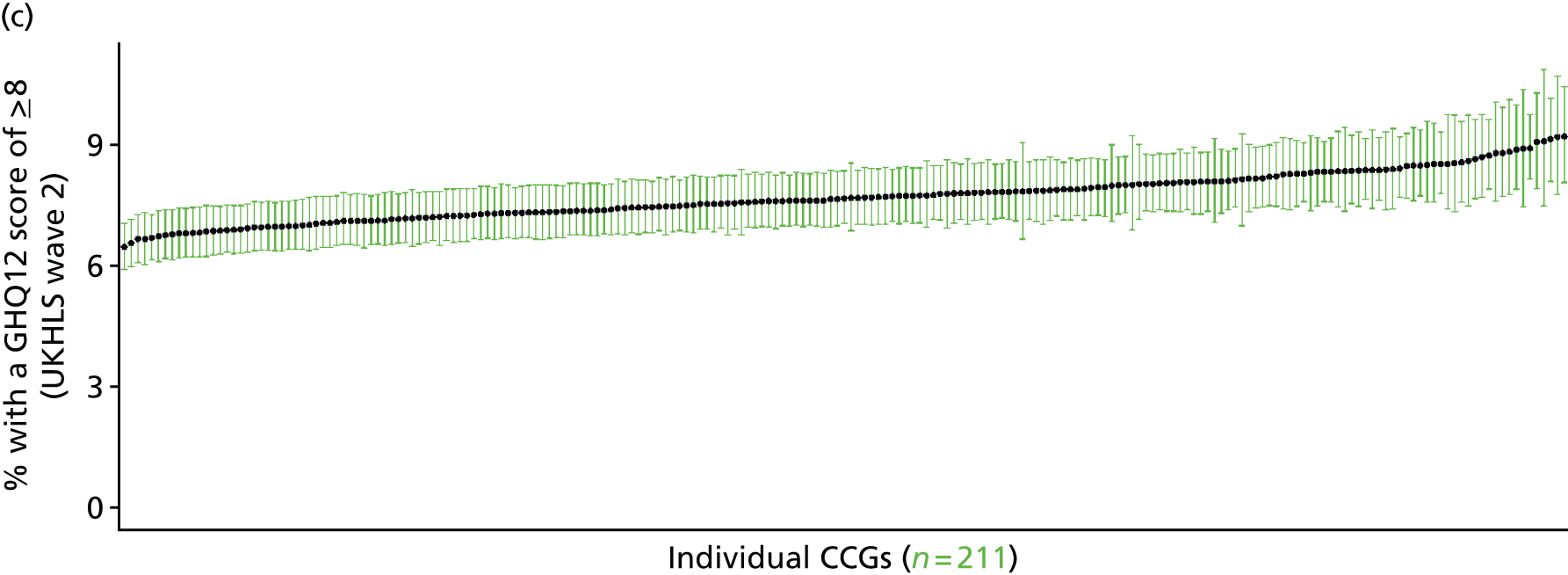
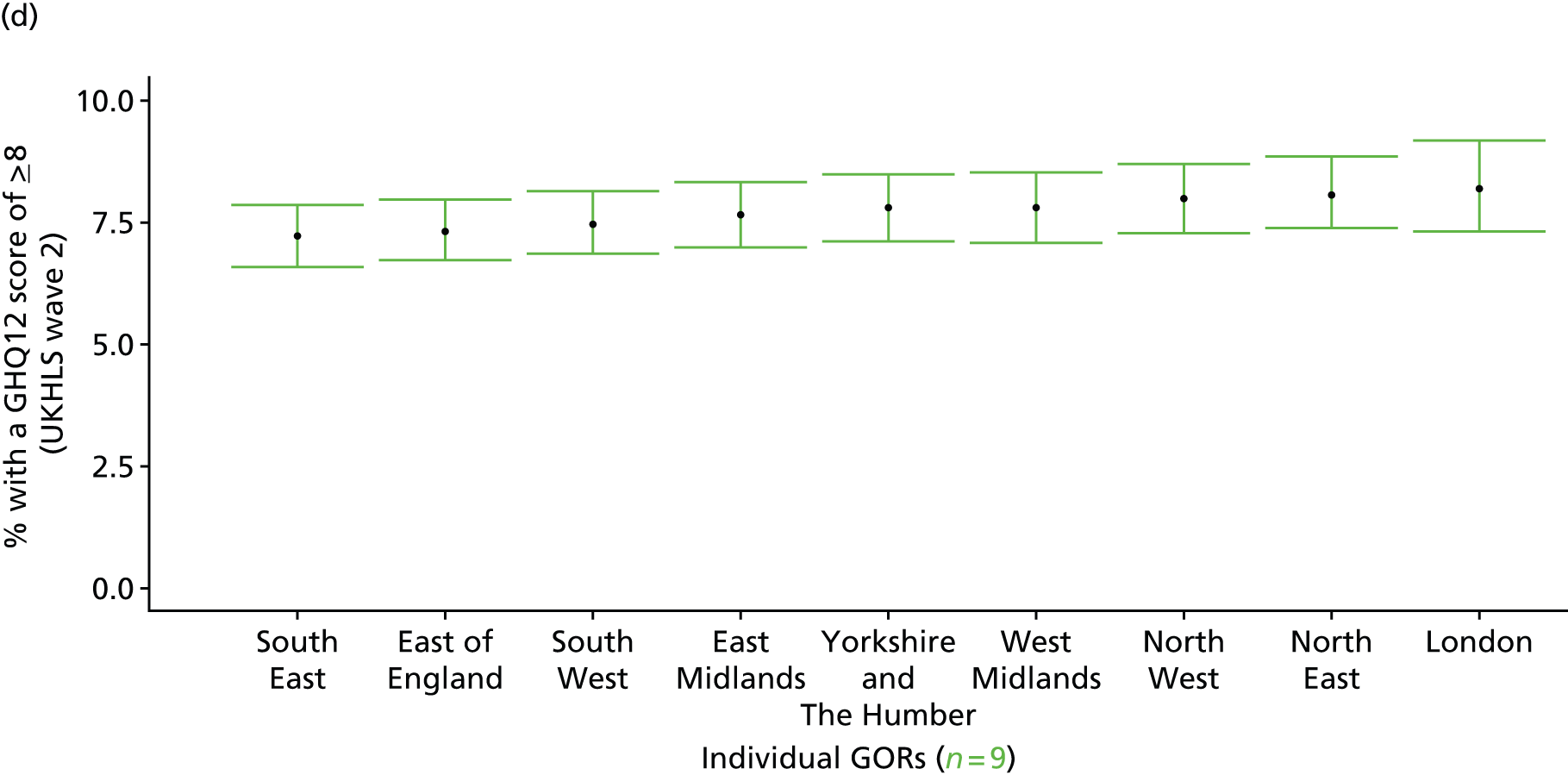
‘Possible’ psychiatric morbidity (12-item General Health Questionnaire score of ≥ 4) or currently prescribed depression/anxiety drugs (UK Household Longitudinal Survey, 2010–12)
FIGURE 159.
Psychiatric morbidity (UKHLS wave 2, GHQ12 score of ≥ 4) or depression/anxiety drugs: LSOA-level map. Contains Ordnance Survey data © Crown copyright and database right 2012.
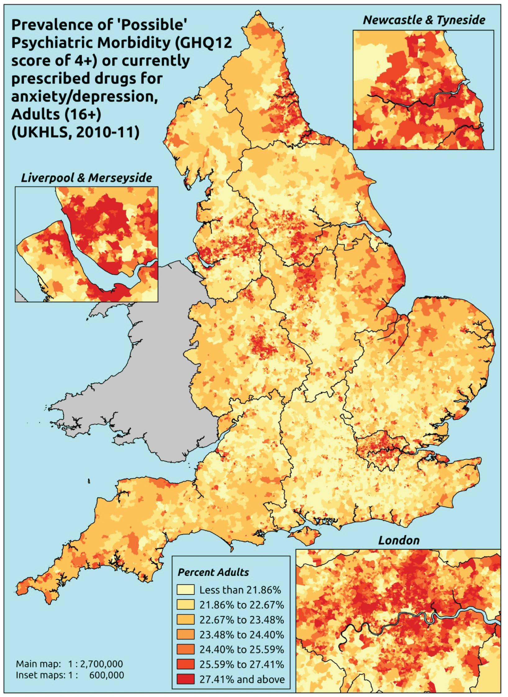
Response variable definition, provenance and prediction
This marker of mental health needs is derived from the 2010–12 second wave of the UKHLS GHQ12 score and questions therein about what medicines the respondent is currently being prescribed. This marker captures respondents with a GHQ12 score of ≥ 4 using the standard 0–12 ‘caseness’ scoring approach or who are currently being prescribed drugs for depression and/or anxiety (BNF 4.1.1–4.1.3 or 4.3.1–4.3.4487). In the literature, a score of ≥ 4 is usually taken as being indicative of ‘possible psychiatric morbidity’. We have no information regarding other forms of treatment for mental health issues. This marker recognises the fact that individuals may return a GHQ12 score of < 4 because they are being receiving medication for anxiety/depression and thus aims to capture underlying levels of ‘possible psychiatric morbidity’. This marker is affected by the fact that (a) other types of medication, and other forms of treatment, are not captured, and (b) any sociodemographic and/or geographic variations in access to, or uptake of, prescribing.
The second wave of the UKHLS data set (n = 31,242) runs from January 2010 to January 2012 and includes multiple household respondents aged ≥ 16 years from across the UK. Here the analytical data set is drawn from the subset of respondents living in England for whom data is available across all model response and predictor variables, namely that they completed the GHQ12, data is available on currently prescribed medication, along with information on age band, sex, ethnicity, LLTI, tenure and the IMD score of the LSOA of residence (n = 7,172). A single randomly selected adult is then drawn from each household, resulting in an analytical data set of 4682 adults aged ≥ 16 years.
| Age band (years) | Females | Age band (years) | Males | ||||
|---|---|---|---|---|---|---|---|
| Does not have condition | Has condition | % | Does not have condition | Has condition | % | ||
| 16–24 | 94 | 41 | 30.4 | 16–24 | 81 | 15 | 15.6 |
| 25–34 | 282 | 123 | 30.4 | 25–34 | 213 | 48 | 18.4 |
| 35–49 | 537 | 245 | 31.3 | 35–49 | 396 | 104 | 20.8 |
| 50–64 | 525 | 243 | 31.6 | 50–64 | 418 | 119 | 22.2 |
| 65–74 | 303 | 95 | 23.9 | 65–74 | 251 | 54 | 17.7 |
| 75–84 | 166 | 54 | 24.5 | 75–84 | 140 | 45 | 24.3 |
| ≥ 85 | 37 | 14 | 27.5 | ≥ 85 | 25 | 14 | 35.9 |
| Females | 1944 | 815 | 29.5 | Males | 1524 | 399 | 20.7 |
| Total (males and females) | 3468 | 1214 | 25.9 | ||||
Model parameters are applied to microsimulated LSOA-level census data to produce estimates of the number (and proportion) of people with treated or untreated ‘possible psychiatric morbidity (i.e. who would score ≥ 4 on the GHQ12 or be currently prescribed drugs for depression and/or anxiety) in each age–sex cohort (and overall) in each of the 32,844 English LSOAs. As discussed in the report, bootstrapping is used to derive 95% CIs for the estimates. These LSOA-level prevalence rate estimates (and 95%CIs) are aggregated into a number of higher geographies; namely MSOAs, LAs, CCGs and regions (GORs). Proportionate attribution is used to restructure the prevalence rate estimates to align with 2001 MSOAs, as well as GP practice populations as defined by the 2011 NHS ADS.
Table 182 summarises how expected prevalence rates vary by age, sex and local deprivation (as measured by the 2010 IMD). There are 6569 LSOAs (with 9,226,227 adults) classified as being in the least deprived quintile; 6568 LSOAs (9,525,344 adults) in the second least deprived quintile; 6568 LSOAs (9,658,444 adults) in the third least deprived quintile; 6568 LSOAs (9,650,576 adults) in the fourth least deprived quintile; and 6568 LSOAs (9,535,167 adults) in the most deprived quintile. Note that, as a general rule, variations in prevalence rates reflect variations in the socioeconomic composition of populations in the different types of LSOA rather than variations in deprivation per se.
| Cohort | Least deprived quintile LSOAs | Second least deprived quintile LSOAs | Third least deprived quintile LSOAs | Fourth least deprived quintile LSOAs | Most deprived quintile LSOAs | All England |
|---|---|---|---|---|---|---|
| Female 16–24 | 25.3 (21.8 to 30.7) | 25.7 (22.3 to 31.1) | 26.3 (22.7 to 31.7) | 27.1 (23.4 to 32.5) | 28.5 (24.4 to 34.0) | 26.8 (23.1 to 32.2) |
| Female 25–34 | 25.3 (23.3 to 27.7) | 25.7 (23.8 to 28.2) | 26.5 (24.3 to 29.0) | 27.5 (25.3 to 30.1) | 29.4 (27.1 to 32.3) | 27.2 (25.0 to 29.7) |
| Female 35–49 | 26.1 (24.8 to 28.0) | 27.0 (25.7 to 29.0) | 28.3 (27.0 to 30.5) | 30.3 (28.9 to 32.7) | 33.5 (31.8 to 36.2) | 29.0 (27.7 to 31.3) |
| Female 50–64 | 26.8 (25.1 to 28.1) | 28.1 (26.6 to 29.6) | 29.8 (28.3 to 31.4) | 32.6 (30.9 to 34.5) | 36.8 (35.2 to 39.3) | 30.5 (28.9 to 32.2) |
| Female 65–74 | 22.9 (21.1 to 25.1) | 24.2 (22.2 to 26.5) | 25.7 (23.7 to 28.2) | 28.2 (25.9 to 31.1) | 31.6 (29.2 to 35.1) | 26.1 (24.1 to 28.7) |
| Female ≥ 75 | 26.5 (24.4 to 30.9) | 27.3 (25.3 to 32.2) | 28.4 (26.2 to 33.5) | 30.0 (27.7 to 35.4) | 32.1 (29.8 to 38.1) | 28.6 (26.6 to 33.7) |
| Females | 25.7 (23.9 to 28.3) | 26.6 (24.8 to 29.4) | 27.8 (25.9 to 30.7) | 29.6 (27.5 to 32.7) | 32.2 (29.9 to 35.8) | 28.4 (26.4 to 31.4) |
| Male 16–24 | 11.9 (8.9 to 15.3) | 12.2 (9.2 to 15.7) | 12.6 (9.6 to 16.2) | 13.2 (10.1 to 17.0) | 14.3 (11.0 to 18.4) | 13.0 (9.8 to 16.7) |
| Male 25–34 | 15.2 (13.3 to 16.9) | 15.7 (13.7 to 17.5) | 16.2 (14.2 to 17.9) | 17.0 (14.9 to 19.0) | 18.9 (16.6 to 21.2) | 16.9 (14.7 to 18.8) |
| Male 35–49 | 16.4 (15.1 to 18.1) | 17.4 (16.0 to 19.1) | 18.6 (17.2 to 20.6) | 20.5 (19.0 to 22.8) | 23.8 (22.0 to 26.4) | 19.4 (17.9 to 21.4) |
| Male 50–64 | 17.8 (16.1 to 19.0) | 19.3 (17.4 to 20.6) | 20.9 (19.0 to 22.4) | 23.6 (21.4 to 25.3) | 27.8 (25.3 to 29.8) | 21.6 (19.6 to 23.1) |
| Male 65–74 | 16.3 (14.5 to 18.0) | 17.7 (15.7 to 19.5) | 19.2 (17.0 to 21.0) | 21.4 (19.0 to 23.7) | 24.7 (22.1 to 27.5) | 19.5 (17.3 to 21.5) |
| Male ≥ 75 | 28.9 (25.5 to 34.3) | 30.1 (26.6 to 35.4) | 31.3 (27.7 to 36.7) | 33.1 (29.4 to 38.8) | 35.5 (31.8 to 41.4) | 31.5 (27.9 to 36.8) |
| Males | 17.5 (15.5 to 19.7) | 18.5 (16.3 to 20.7) | 19.3 (17.2 to 21.7) | 20.6 (18.3 to 23.2) | 23.0 (20.5 to 25.9) | 19.8 (17.6 to 22.2) |
| All | 21.8 (21.2 to 22.5) | 22.7 (22.2 to 23.6) | 23.7 (23.1 to 24.7) | 25.2 (24.5 to 26.4) | 27.7 (26.7 to 29.4) | 24.2 (23.5 to 25.3) |
| Factor (reference group) | Model coefficients | 95% CI | ||
|---|---|---|---|---|
| Estimate | SE | 2.5% CI | 97.50% | |
| (Intercept) | –1.39974 | 0.17872 | –1.75004 | –1.04944 |
| Age (16–24 years) | ||||
| 25–34 years | 0.08149 | 0.18466 | –0.28045 | 0.44343 |
| 35–49 years | 0.09218 | 0.17534 | –0.25149 | 0.43584 |
| 50–64 years | –0.01860 | 0.17741 | –0.36632 | 0.32912 |
| 65–74 years | –0.47408 | 0.19280 | –0.85197 | –0.09619 |
| 75–84 years | –0.48659 | 0.20849 | –0.89522 | –0.07795 |
| ≥ 85 years | –0.20392 | 0.29267 | –0.77756 | 0.36971 |
| Sex (females) | ||||
| Males | –0.62948 | 0.09453 | –0.81476 | –0.44421 |
| Ethnicity (white) | ||||
| Mixed | 0.01401 | 0.39694 | –0.76399 | 0.79201 |
| Black | –0.06709 | 0.21538 | –0.48924 | 0.35506 |
| Asian | 0.01289 | 0.27464 | –0.52540 | 0.55119 |
| Other | 0.84902 | 0.36409 | 0.13540 | 1.56264 |
| LLTI (no LTTI) | ||||
| LLTI | 1.08426 | 0.11066 | 0.86737 | 1.30116 |
| Tenure (owner–occupier) | ||||
| Social rent | 0.42582 | 0.12874 | 0.17348 | 0.67816 |
| Private rent or other tenure | 0.03353 | 0.13528 | –0.23162 | 0.29868 |
| LSOA IMD deprivation score | ||||
| IMD score | 0.00788 | 0.00253 | 0.00292 | 0.01284 |
| Interaction effects | ||||
| Male and LLTI | 0.40873 | 0.15318 | 0.10850 | 0.70897 |
| LLTI and social rent | 0.07156 | 0.18255 | –0.28625 | 0.42936 |
| LLTI and private rent or other tenure | 0.52148 | 0.24559 | 0.04012 | 1.00283 |
FIGURE 160.
Parameter plots: psychiatric morbidity (UKHLS wave 2, GHQ12 score of ≥ 4) or depression/anxiety drugs.

FIGURE 161.
Psychiatric morbidity (UKHLS wave 2, GHQ12 score of ≥ 4) or depression/anxiety drugs: individual estimates and their 95% CIs. (a) MSOAs; (b) LAs; (c) CCGs; and (d) regions (GORs).
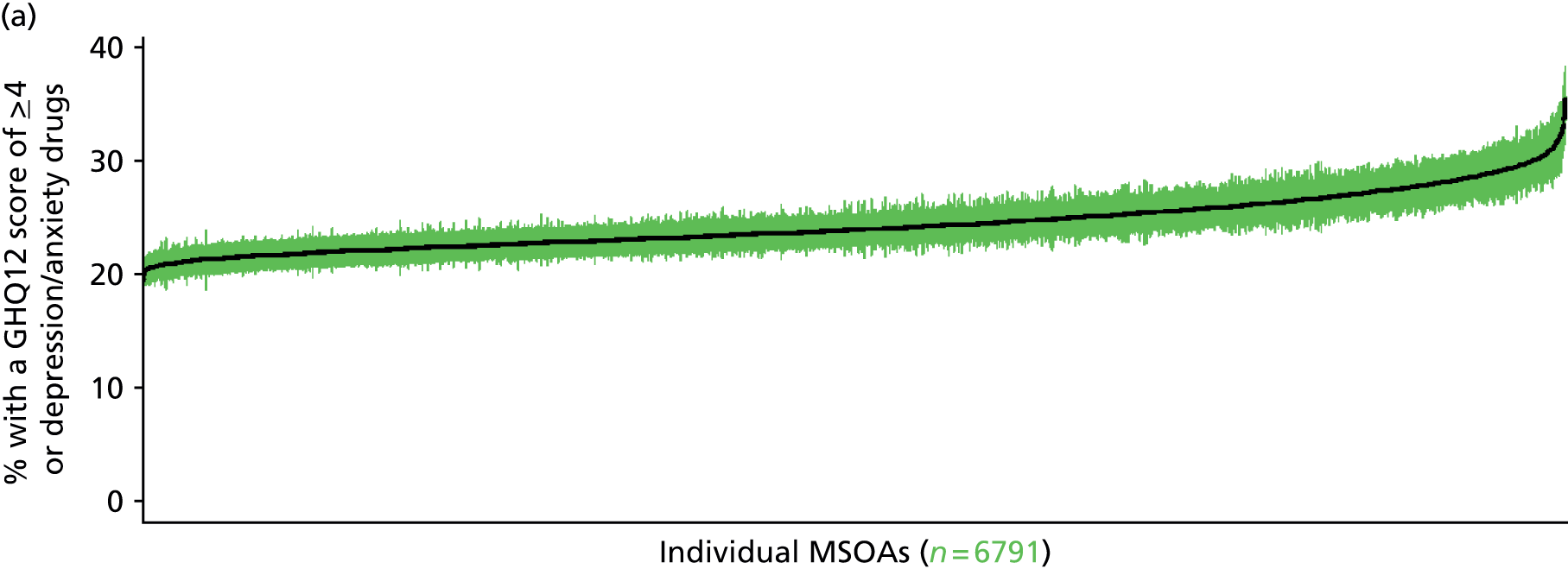
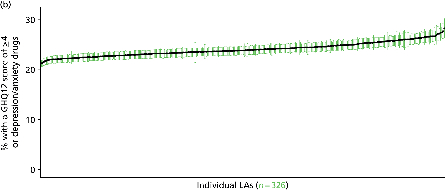
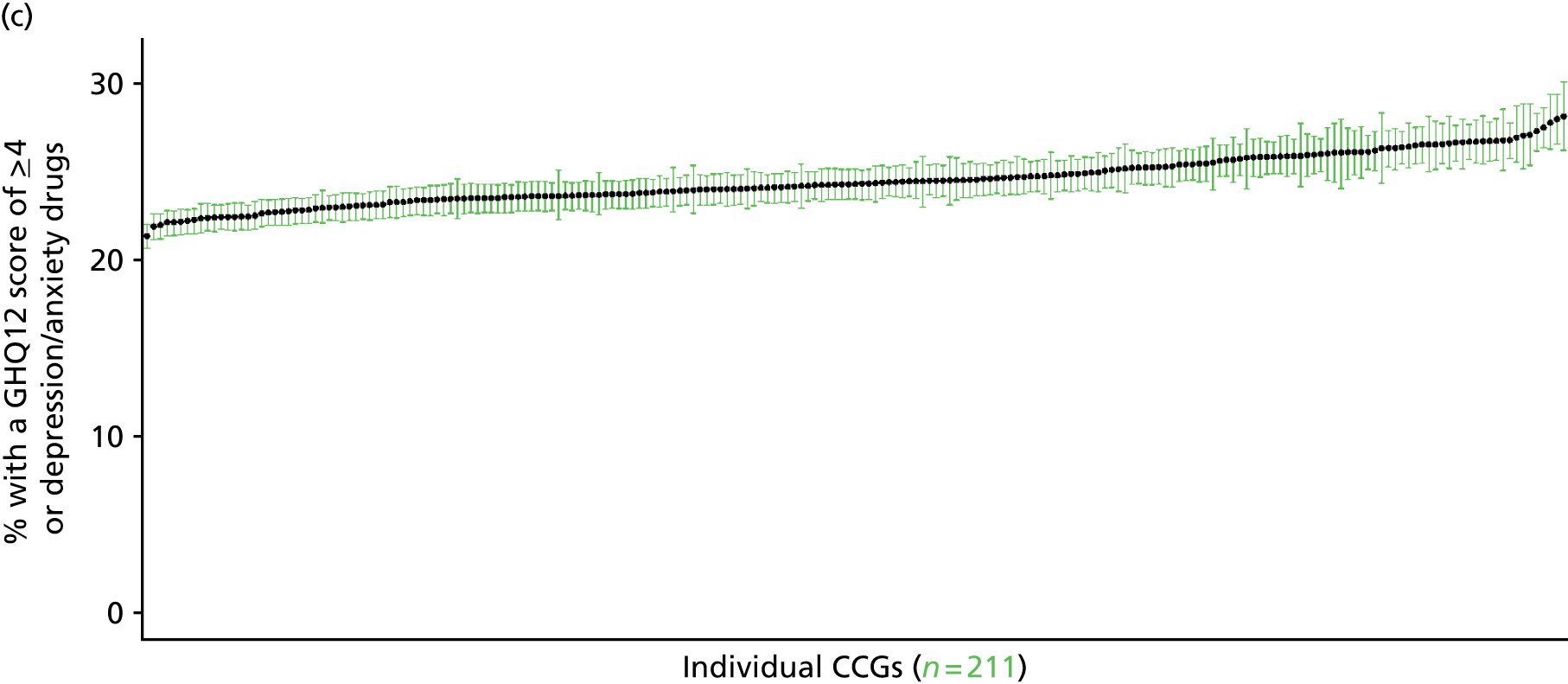
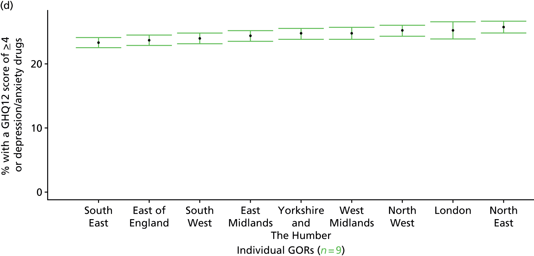
‘Probable’ psychiatric morbidity (12-item General Health Questionnaire score ≥ 6) or currently prescribed depression/anxiety drugs (UK Household Longitudinal Survey, wave 2, 2010–12)
FIGURE 162.
Psychiatric morbidity (UKHLS wave 2, GHQ12 ≥ 6) or depression/anxiety drugs: LSOA-level map. Contains Ordnance Survey data © Crown copyright and database right 2012.

Response variable definition, provenance and prediction
This marker of mental health needs is derived from the 2010–12 second wave of the UKHLS GHQ12 questionnaire score and questions therein about what medicines the respondent is currently being prescribed. This marker captures respondents with a GHQ12 score of ≥ 6 using the standard 0–12 ‘caseness’ scoring approach or who are currently being prescribed drugs for depression and/or anxiety (BNF 4.1.1–4.1.3 or 4.3.1–4.3.4487). In the literature, a score of ≥ 4 is usually taken as being indicative of ‘possible psychiatric morbidity’, but occasionally a ≥ 6 threshold is used. For convenience (and without clinical justification) we describe this as a marker of ‘probable psychiatric morbidity’ – to distinguish this marker from those using the standard ≥ 4 threshold (‘possible psychiatric morbidity’) and the higher ≥ 8 threshold (‘psychiatric morbidity’). We have no information regarding other forms of treatment for mental health issues. This marker recognises the fact that individuals may return a GHQ12 score of < 6 because they are being receiving medication for anxiety/depression and thus aims to capture underlying levels of ‘probable psychiatric morbidity’. This marker is affected by the fact that (a) other types of medication, and other forms of treatment, are not captured, and (b) any sociodemographic and/or geographic variations in access to, or uptake of, prescribing.
The second wave of the UKHLS data set (n = 31,242) runs from January 2010 to January 2012 and includes multiple household respondents aged ≥ 16 years from across the UK. Here the analytical data set is drawn from the subset of respondents living in England for whom data are available across all model response and predictor variables, namely that they completed the GHQ12 questionnaire, data are available on currently prescribed medication, along with information on age band, sex, ethnicity, LLTI, tenure and the IMD score of the LSOA of residence (n = 7172). A single randomly selected adult is then drawn from each household, resulting in an analytical data set of 4682 adults aged ≥ 16 years.
| Age band (years) | Females | Age band (years) | Males | ||||
|---|---|---|---|---|---|---|---|
| Does not have condition | Has condition | % | Does not have condition | Has condition | % | ||
| 16–24 | 102 | 33 | 24.4 | 16–24 | 88 | 8 | 8.3 |
| 25–34 | 314 | 91 | 22.5 | 25–34 | 221 | 40 | 15.3 |
| 35–49 | 591 | 191 | 24.4 | 35–49 | 414 | 86 | 17.2 |
| 50–64 | 572 | 196 | 25.5 | 50–64 | 440 | 97 | 18.1 |
| 65–74 | 321 | 77 | 19.3 | 65–74 | 255 | 50 | 16.4 |
| 75–84 | 180 | 40 | 18.2 | 75–84 | 148 | 37 | 20.0 |
| ≥ 85 | 40 | 11 | 21.6 | ≥ 85 | 25 | 14 | 35.9 |
| Females | 2120 | 639 | 23.2 | Males | 1591 | 332 | 17.3 |
| Total (males and females) | 3711 | 971 | 20.7 | ||||
Model parameters are applied to microsimulated LSOA-level census data to produce estimates of the number (and proportion) of people with treated or untreated ‘probable psychiatric morbidity (i.e. who would score ≥ 6 on the GHQ12 or be currently prescribed drugs for depression and/or anxiety) in each age–sex cohort (and overall) in each of the 32,844 English LSOAs. As discussed in the report, bootstrapping is used to derive 95% CIs for the estimates. These LSOA-level prevalence rate estimates (and 95% CIs) are aggregated into a number of higher geographies; namely MSOAs, LAs, CCGs and regions (GORs). Proportionate attribution is used to restructure the prevalence rate estimates to align with 2001 MSOAs, as well as GP practice populations as defined by the 2011 NHS ADS.
Table 185 summarises how expected prevalence rates vary by age, sex and local deprivation (as measured by the 2010 IMD). There are 6569 LSOAs (with 9,226,227 adults) classified as being in the least deprived quintile; 6568 LSOAs (9,525,344 adults) in the second least deprived quintile; 6568 LSOAs (9,658,444 adults) in the third least deprived quintile; 6568 LSOAs (9,650,576 adults) in the fourth least deprived quintile; and 6568 LSOAs (9,535,167 adults) in the most deprived quintile. Note that, as a general rule, variations in prevalence rates reflect variations in the socioeconomic composition of populations in the different types of LSOA rather than variations in deprivation per se.
| Cohort | Least deprived quintile LSOAs | Second least deprived quintile LSOAs | Third least deprived quintile LSOAs | Fourth least deprived quintile LSOAs | Most deprived quintile LSOAs | All England |
|---|---|---|---|---|---|---|
| Female 16–24 | 18.9 (16.1 to 22.1) | 19.4 (16.5 to 22.6) | 19.7 (16.9 to 23.2) | 20.3 (17.4 to 23.8) | 21.3 (18.2 to 25.0) | 20.1 (17.2 to 23.5) |
| Female 25–34 | 17.4 (16.2 to 19.3) | 17.9 (16.6 to 19.8) | 18.4 (17.0 to 20.3) | 19.2 (17.8 to 21.3) | 20.7 (19.0 to 22.9) | 18.9 (17.5 to 21.0) |
| Female 35–49 | 19.6 (18.3 to 20.9) | 20.5 (19.2 to 21.9) | 21.5 (20.3 to 23.0) | 23.2 (21.8 to 24.9) | 25.8 (24.2 to 27.9) | 22.1 (20.8 to 23.7) |
| Female 50–64 | 20.7 (19.6 to 22.4) | 22.1 (20.9 to 23.8) | 23.5 (22.3 to 25.4) | 25.8 (24.4 to 27.8) | 29.6 (27.8 to 32.0) | 24.1 (22.8 to 26.0) |
| Female 65–74 | 18.2 (16.5 to 20.1) | 19.2 (17.4 to 21.3) | 20.2 (18.4 to 22.6) | 21.9 (19.9 to 24.7) | 24.6 (22.3 to 27.7) | 20.5 (18.7 to 23.0) |
| Female ≥ 75 | 16.6 (15.2 to 19.4) | 17.0 (15.5 to 19.9) | 17.6 (15.9 to 20.4) | 18.2 (16.5 to 21.3) | 19.4 (17.5 to 22.5) | 17.7 (16.1 to 20.6) |
| Females | 19.0 (17.5 to 20.9) | 19.8 (18.3 to 21.8) | 20.6 (19.0 to 22.8) | 21.9 (20.2 to 24.3) | 24.0 (22.1 to 26.7) | 21.1 (19.4 to 23.3) |
| Male 16–24 | 5.9 (4.2 to 7.9) | 6.0 (4.4 to 8.1) | 6.2 (4.6 to 8.3) | 6.6 (4.8 to 8.7) | 7.1 (5.1 to 9.6) | 6.4 (4.7 to 8.5) |
| Male 25–34 | 12.1 (10.5 to 13.6) | 12.5 (10.9 to 14.0) | 12.9 (11.2 to 14.5) | 13.7 (11.8 to 15.3) | 15.2 (13.2 to 17.1) | 13.5 (11.7 to 15.1) |
| Male 35–49 | 13.1 (12.1 to 14.4) | 14.0 (12.9 to 15.5) | 15.2 (13.9 to 16.8) | 16.9 (15.5 to 18.8) | 19.9 (18.2 to 22.1) | 15.9 (14.5 to 17.5) |
| Male 50–64 | 13.8 (12.2 to 14.8) | 15.2 (13.5 to 16.4) | 16.8 (14.9 to 18.1) | 19.1 (17.1 to 20.9) | 23.0 (20.5 to 25.2) | 17.3 (15.4 to 18.8) |
| Male 65–74 | 14.9 (13.4 to 16.7) | 16.2 (14.6 to 18.1) | 17.4 (15.8 to 19.5) | 19.4 (17.6 to 21.9) | 22.4 (20.4 to 25.3) | 17.7 (16.1 to 19.8) |
| Male ≥ 75 | 22.8 (20.2 to 26.4) | 23.6 (20.8 to 27.2) | 24.4 (21.4 to 28.1) | 25.4 (22.5 to 29.2) | 27.1 (24.0 to 30.7) | 24.5 (21.6 to 28.1) |
| Males | 13.7 (12.1 to 15.3) | 14.5 (12.9 to 16.3) | 15.2 (13.5 to 17.1) | 16.2 (14.4 to 18.3) | 18.2 (16.1 to 20.6) | 15.6 (13.8 to 17.5) |
| All | 16.4 (15.9 to 16.9) | 17.2 (16.7 to 17.8) | 18.0 (17.4 to 18.7) | 19.1 (18.4 to 20.0) | 21.2 (20.2 to 22.3) | 18.4 (17.7 to 19.1) |
| Factor (reference group) | Model coefficients | 95% CI | ||
|---|---|---|---|---|
| Estimate | SE | 2.5% CI | 97.50% | |
| (Intercept) | –1.68620 | 0.22691 | –2.13094 | –1.24145 |
| Age (16–24 years) | ||||
| 25–34 years | –0.15004 | 0.25038 | –0.64078 | 0.34070 |
| 35–49 years | –0.04669 | 0.23762 | –0.51242 | 0.41905 |
| 50–64 years | –0.15123 | 0.24327 | –0.62803 | 0.32558 |
| 65–74 years | –0.48139 | 0.27698 | –1.02426 | 0.06149 |
| 75–84 years | –0.44614 | 0.32867 | –1.09033 | 0.19804 |
| ≥ 85 years | 0.14258 | 0.47508 | –0.78857 | 1.07374 |
| Sex (females) | ||||
| Males | –1.44101 | 0.44045 | –2.30429 | –0.57773 |
| Ethnicity (white) | ||||
| Mixed | –0.17268 | 0.44911 | –1.05294 | 0.70757 |
| Black | –0.54372 | 0.26536 | –1.06383 | –0.02361 |
| Asian | –0.11097 | 0.29761 | –0.69429 | 0.47236 |
| Other | 0.54586 | 0.39108 | –0.22066 | 1.31238 |
| LLTI (no LTTI) | ||||
| LLTI | 1.04535 | 0.51441 | 0.03710 | 2.05359 |
| Tenure (owner–occupier) | ||||
| Social rent | 0.53099 | 0.10433 | 0.32651 | 0.73547 |
| Private rent or other tenure | 0.32404 | 0.12062 | 0.08761 | 0.56046 |
| LSOA IMD deprivation score | ||||
| IMD score | 0.00866 | 0.00269 | 0.00338 | 0.01394 |
| Interaction effects | ||||
| Male and LLTI | 0.49223 | 0.17211 | 0.15490 | 0.82957 |
| 25–34 years and male | 0.90736 | 0.49157 | –0.05611 | 1.87083 |
| 35–49 years and male | 0.86677 | 0.46568 | –0.04595 | 1.77950 |
| 50–64 years and male | 0.75529 | 0.46664 | –0.15932 | 1.66990 |
| 65–74 years and male | 0.91647 | 0.49107 | –0.04603 | 1.87897 |
| 75–84 years and male | 1.26521 | 0.51619 | 0.25348 | 2.27693 |
| ≥ 85 years and male | 2.00439 | 0.65491 | 0.72077 | 3.28801 |
| 25–34 years and LLTI | 0.29583 | 0.57918 | –0.83935 | 1.43102 |
| 35–49 years and LLTI | 0.18311 | 0.53490 | –0.86529 | 1.23151 |
| 50–64 years and LLTI | 0.22086 | 0.53075 | –0.81940 | 1.26113 |
| 65–74 years and LLTI | 0.03021 | 0.55133 | –1.05040 | 1.11082 |
| 75–84 years and LLTI | –0.46440 | 0.57935 | –1.59992 | 0.67112 |
| ≥ 85 years and LLTI | –1.34386 | 0.70379 | –2.72329 | 0.03557 |
FIGURE 163.
Parameter plots: psychiatric morbidity (UKHLS wave 2, GHQ12 score of ≥ 6) or depression/anxiety drugs.

FIGURE 164.
Psychiatric morbidity (UKHLS wave 2, GHQ12 score of ≥ 6) or depression/anxiety drugs: individual estimates and their 95% CIs. (a) MSOAs; (b) LAs; (c) CCGs; and (d) regions (GORs).

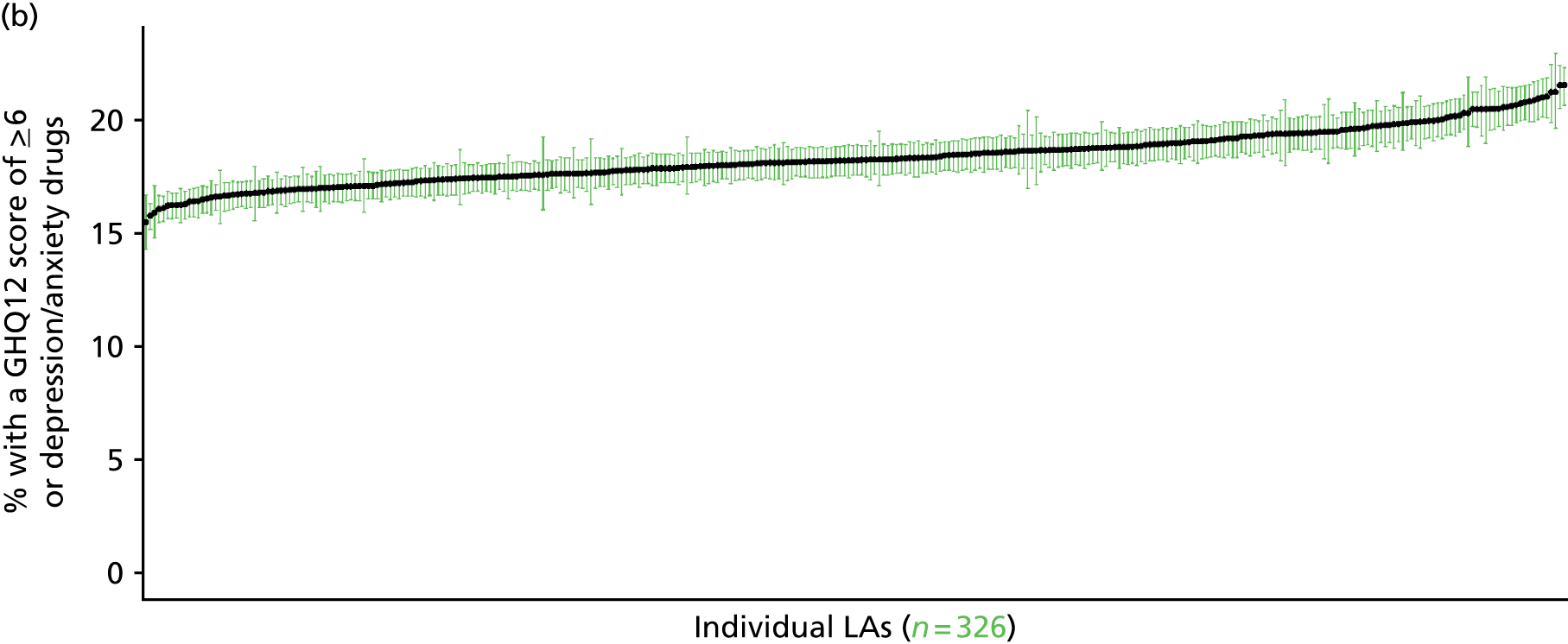
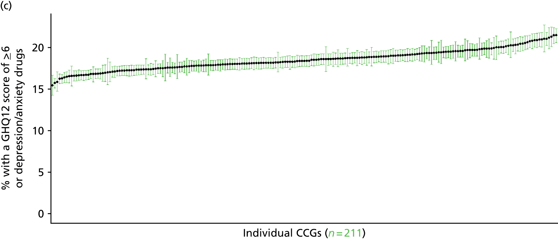

Psychiatric morbidity (12-item General Health Questionnaire score of ≥ 8) or currently prescribed depression/anxiety drugs (UK Household Longitudinal Survey, wave 2, 2010–12)
FIGURE 165.
Psychiatric morbidity (UKHLS GHQ12 score of ≥ 8) or depression/anxiety drugs: LSOA-level map. Contains Ordnance Survey data © Crown copyright and database right 2012.

Response variable definition, provenance and prediction
This marker of mental health needs is derived from the 2010–12 second wave of the UKHLS GHQ12 score and questions therein about what medicines the respondent is currently being prescribed. This marker captures respondents with a GHQ12 score of ≥ 8 using the standard 0–12 ‘caseness’ scoring approach or who are currently being prescribed drugs for depression and/or anxiety (BNF 4.1.1–4.1.3 or 4.3.1–4.3.4487). In the literature, a score of ≥ 4 is usually taken as being indicative of ‘possible psychiatric morbidity’, but occasionally ≥ 6 or ≥ 8 thresholds are used. For convenience (and without clinical justification) we describe this as a marker of ‘psychiatric morbidity’ – to distinguish it from the standard ≥ 4 threshold (‘possible psychiatric morbidity’) and the ≥ 6 threshold (‘probable psychiatric morbidity’). We have no information regarding other forms of treatment for mental health issues. This marker recognises the fact that individuals may return a GHQ12 score of < 8 because they are being receiving medication for anxiety/depression and thus aims to capture underlying levels of ‘probable psychiatric morbidity’. This marker is affected by the fact that (a) other types of medication, and other forms of treatment, are not captured, and (b) any sociodemographic and/or geographic variations in access to, or uptake of, prescribing.
The second wave of the UKHLS data set (n = 31,242) runs from January 2010 to January 2012 and includes multiple household respondents aged ≥ 16 years from across the UK. Here the analytical data set is drawn from the subset of respondents living in England for whom data are available across all model response and predictor variables, namely that they completed the GHQ12, data are available on currently prescribed medication, along with information on age band, sex, ethnicity, LLTI, tenure and the IMD score of the LSOA of residence (n = 7172). A single randomly selected adult is then drawn from each household, resulting in an analytical data set of 4682 adults aged ≥ 16 years.
| Age band (years) | Females | Age band (years) | Males | ||||
|---|---|---|---|---|---|---|---|
| Does not have condition | Has condition | % | Does not have condition | Has condition | % | ||
| 16–24 | 110 | 25 | 18.5 | 16–24 | 91 | 5 | 5.2 |
| 25–34 | 332 | 73 | 18.0 | 25–34 | 233 | 28 | 10.7 |
| 35–49 | 629 | 153 | 19.6 | 35–49 | 430 | 70 | 14.0 |
| 50–64 | 611 | 157 | 20.4 | 50–64 | 453 | 84 | 15.6 |
| 65–74 | 335 | 63 | 15.8 | 65–74 | 262 | 43 | 14.1 |
| 75–84 | 189 | 31 | 14.1 | 75–84 | 154 | 31 | 16.8 |
| ≥ 85 | 41 | 10 | 19.6 | ≥ 85 | 31 | 8 | 20.5 |
| Females | 2247 | 512 | 18.6 | Males | 1654 | 269 | 14.0 |
| Total (males and females) | 3901 | 781 | 16.7 | ||||
Model parameters are applied to microsimulated LSOA-level census data to produce estimates of the number (and proportion) of people with treated or untreated ‘psychiatric morbidity (i.e. who would score ≥ 8 on the GHQ12 or be currently prescribed drugs for depression and/or anxiety) in each age–sex cohort (and overall) in each of the 32,844 English LSOAs. As discussed in the report, bootstrapping is used to derive 95% CIs for the estimates. These LSOA-level prevalence rate estimates (and 95% CIs) are aggregated into a number of higher geographies; namely MSOAs, LAs, CCGs and regions (GORs). Proportionate attribution is used to restructure the prevalence rate estimates to align with 2001 MSOAs, as well as GP practice populations as defined by the 2011 NHS ADS.
Table 188 summarises how expected prevalence rates vary by age, sex and local deprivation (as measured by the 2010 IMD). There are 6569 LSOAs (with 9,226,227 adults) classified as being in the least deprived quintile; 6568 LSOAs (9,525,344 adults) in the second least deprived quintile; 6568 LSOAs (9,658,444 adults) in the third least deprived quintile; 6568 LSOAs (9,650,576 adults) in the fourth least deprived quintile; and 6568 LSOAs (9,535,167 adults) in the most deprived quintile. Note that, as a general rule, variations in prevalence rates reflect variations in the socioeconomic composition of populations in the different types of LSOA rather than variations in deprivation per se.
| Cohort | Least deprived quintile LSOAs | Second least deprived quintile LSOAs | Third least deprived quintile LSOAs | Fourth least deprived quintile LSOAs | Most deprived quintile LSOAs | All England |
|---|---|---|---|---|---|---|
| Female 16–24 | 12.3 (10.4 to 14.3) | 12.5 (10.5 to 14.5) | 12.6 (10.6 to 14.5) | 12.8 (10.9 to 14.8) | 13.4 (11.3 to 15.5) | 12.8 (10.8 to 14.7) |
| Female 25–34 | 14.1 (13.0 to 15.2) | 14.4 (13.3 to 15.5) | 14.7 (13.5 to 15.8) | 15.3 (14.0 to 16.5) | 16.5 (15.0 to 17.8) | 15.2 (13.9 to 16.3) |
| Female 35–49 | 15.7 (15.1 to 16.9) | 16.6 (15.8 to 17.7) | 17.4 (16.7 to 18.8) | 18.9 (18.0 to 20.2) | 21.2 (20.2 to 23.0) | 18.0 (17.2 to 19.4) |
| Female 50–64 | 16.6 (15.5 to 17.6) | 17.6 (16.6 to 18.6) | 18.7 (17.5 to 19.8) | 20.5 (19.3 to 21.9) | 23.8 (22.1 to 25.4) | 19.2 (18.1 to 20.3) |
| Female 65–74 | 15.3 (14.0 to 16.8) | 16.2 (14.8 to 17.8) | 17.3 (15.7 to 18.9) | 18.8 (17.0 to 20.9) | 21.4 (19.3 to 24.1) | 17.5 (15.9 to 19.3) |
| Female ≥ 75 | 15.2 (14.1 to 17.4) | 15.7 (14.5 to 18.0) | 16.2 (15.0 to 18.7) | 17.0 (15.7 to 19.8) | 18.3 (16.9 to 21.4) | 16.4 (15.2 to 18.9) |
| Females | 15.3 (14.2 to 16.7) | 15.9 (14.8 to 17.4) | 16.5 (15.3 to 18.1) | 17.5 (16.2 to 19.2) | 19.3 (17.7 to 21.2) | 16.9 (15.7 to 18.5) |
| Male 16–24 | 7.7 (6.3 to 9.0) | 7.9 (6.5 to 9.3) | 8.1 (6.7 to 9.6) | 8.3 (6.9 to 10.1) | 9.0 (7.4 to 10.9) | 8.3 (6.9 to 9.9) |
| Male 25–34 | 9.3 (8.2 to 10.1) | 9.6 (8.5 to 10.4) | 9.9 (8.8 to 10.7) | 10.5 (9.3 to 11.4) | 12.1 (10.6 to 13.0) | 10.5 (9.3 to 11.3) |
| Male 35–49 | 10.3 (9.6 to 11.0) | 11.3 (10.5 to 12.1) | 12.3 (11.5 to 13.2) | 14.0 (13.0 to 15.1) | 17.1 (15.7 to 18.5) | 13.0 (12.2 to 14.0) |
| Male 50–64 | 12.0 (11.0 to 12.7) | 13.4 (12.3 to 14.2) | 14.9 (13.6 to 15.8) | 17.2 (15.9 to 18.5) | 21.2 (19.5 to 22.9) | 15.5 (14.3 to 16.5) |
| Male 65–74 | 12.8 (11.6 to 14.2) | 14.2 (12.8 to 15.7) | 15.4 (14.0 to 17.2) | 17.5 (15.9 to 19.6) | 20.8 (18.6 to 23.3) | 15.8 (14.4 to 17.6) |
| Male ≥ 75 | 14.0 (12.6 to 16.0) | 14.8 (13.3 to 16.8) | 15.3 (13.8 to 17.7) | 16.4 (14.8 to 19.2) | 18.0 (16.2 to 21.1) | 15.5 (14.0 to 17.9) |
| Males | 11.1 (10.0 to 12.1) | 12.0 (10.8 to 13.1) | 12.7 (11.5 to 13.9) | 13.7 (12.5 to 15.2) | 16.0 (14.4 to 17.7) | 13.1 (11.9 to 14.4) |
| All | 13.3 (12.9 to 13.8) | 14.0 (13.6 to 14.5) | 14.7 (14.2 to 15.3) | 15.7 (15.1 to 16.3) | 17.7 (16.9 to 18.5) | 15.1 (14.6 to 15.7) |
| Factor (reference group) | Model coefficients | 95% CI | ||
|---|---|---|---|---|
| Estimate | SE | 2.5% CI | 97.50% | |
| (Intercept) | –2.11468 | 0.24507 | –2.59502 | –1.63434 |
| Age (16–24 years) | ||||
| 25–34 years | 0.07316 | 0.25799 | –0.43250 | 0.57882 |
| 35–49 years | 0.16775 | 0.24659 | –0.31557 | 0.65107 |
| 50–64 years | 0.10954 | 0.25248 | –0.38532 | 0.60439 |
| 65–74 years | –0.15840 | 0.28465 | –0.71632 | 0.39952 |
| 75–84 years | –0.01828 | 0.33399 | –0.67290 | 0.63633 |
| ≥ 85 years | 1.07861 | 0.42293 | 0.24967 | 1.90755 |
| Sex (females) | ||||
| Males | –0.65915 | 0.12056 | –0.89544 | –0.42286 |
| Ethnicity (white) | ||||
| Mixed | –0.08027 | 0.47947 | –1.02004 | 0.85950 |
| Black | –0.91361 | 0.33322 | –1.56673 | –0.26050 |
| Asian | –0.12705 | 0.33138 | –0.77656 | 0.52246 |
| Other | 0.57534 | 0.41784 | –0.24362 | 1.39431 |
| LLTI (no LTTI) | ||||
| LLTI | 0.78214 | 0.54080 | –0.27782 | 1.84211 |
| Tenure (owner–occupier) | ||||
| Social rent | 0.39576 | 0.15677 | 0.08849 | 0.70302 |
| Private rent or other tenure | 0.11049 | 0.17083 | –0.22434 | 0.44532 |
| LSOA IMD deprivation score | ||||
| IMD score | 0.00586 | 0.00293 | 0.00011 | 0.0116 |
| Interaction effects | ||||
| Male and LLTI | 0.73400 | 0.17724 | 0.38662 | 1.08138 |
| 25–34 years and LLTI | 0.57259 | 0.59649 | –0.59652 | 1.74171 |
| 35–49 years and LLTI | 0.38225 | 0.55188 | –0.69943 | 1.46394 |
| 50–64 years and LLTI | 0.21091 | 0.54868 | –0.86450 | 1.28631 |
| 65–74 years and LLTI | 0.10867 | 0.57301 | –1.01442 | 1.23177 |
| 75–84 years and LLTI | –0.35462 | 0.60674 | –1.54383 | 0.83459 |
| ≥ 85 years and LLTI | –1.93496 | 0.75789 | –3.42043 | –0.44949 |
| LLTI and social rent | 0.32577 | 0.20701 | –0.07997 | 0.73150 |
| LLTI and private rent or other tenure | 0.58345 | 0.27385 | 0.04670 | 1.12020 |
FIGURE 166.
Parameter plots: psychiatric morbidity (UKHLS GHQ12 score of ≥ 8) or depression/anxiety drugs.
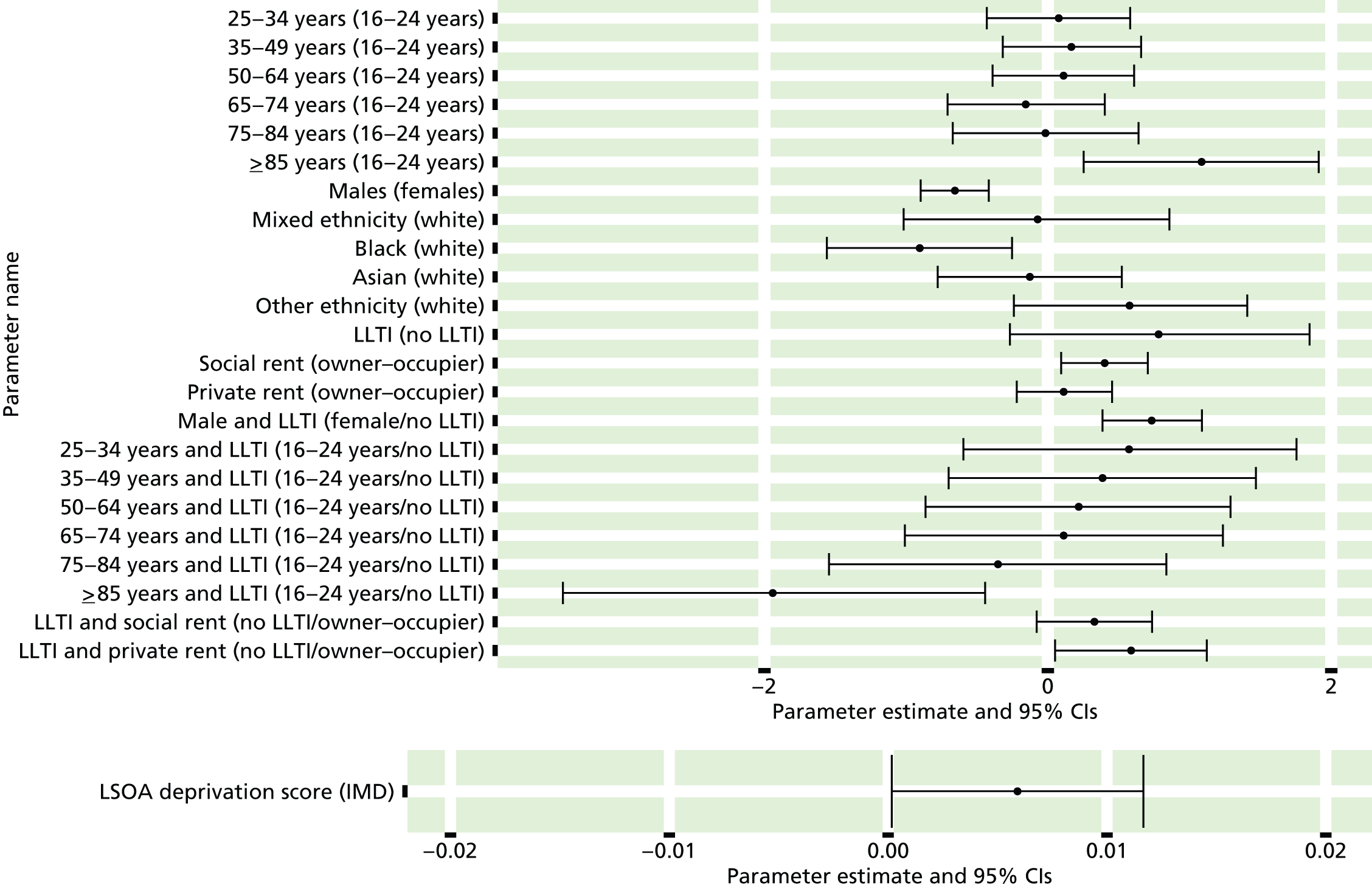
FIGURE 167.
Psychiatric morbidity (UKHLS wave 2 GHQ12 score of ≥ 8) or depression/anxiety drugs: individual estimates and their 95% CIs. (a) MSOAs; (b) LAs; (c) CCGs; and (d) regions (GORs).

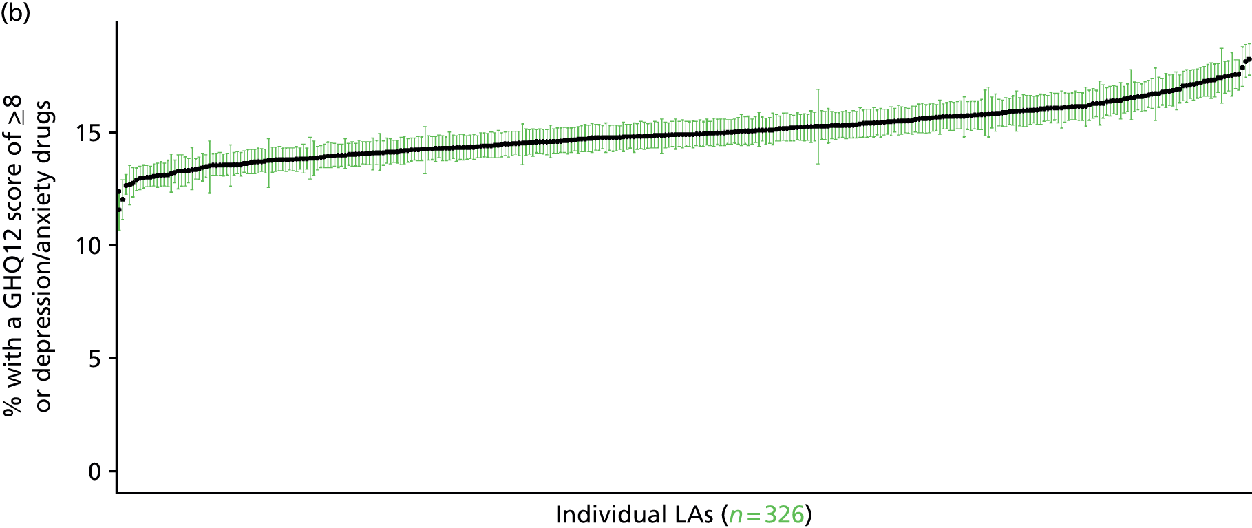
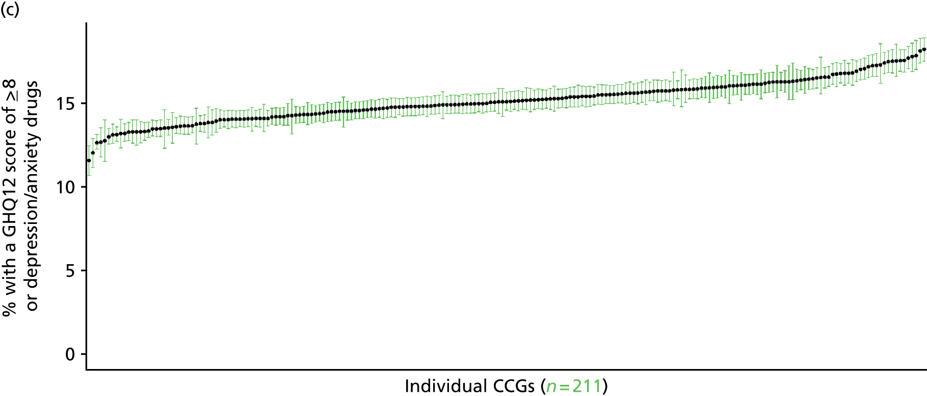

Diagnosed with clinical depression (UK Household Longitudinal Survey, wave 1, 2009–10)
FIGURE 168.
Diagnosed with clinical depression: LSOA-level map. Contains Ordnance Survey data © Crown copyright and database right 2012.
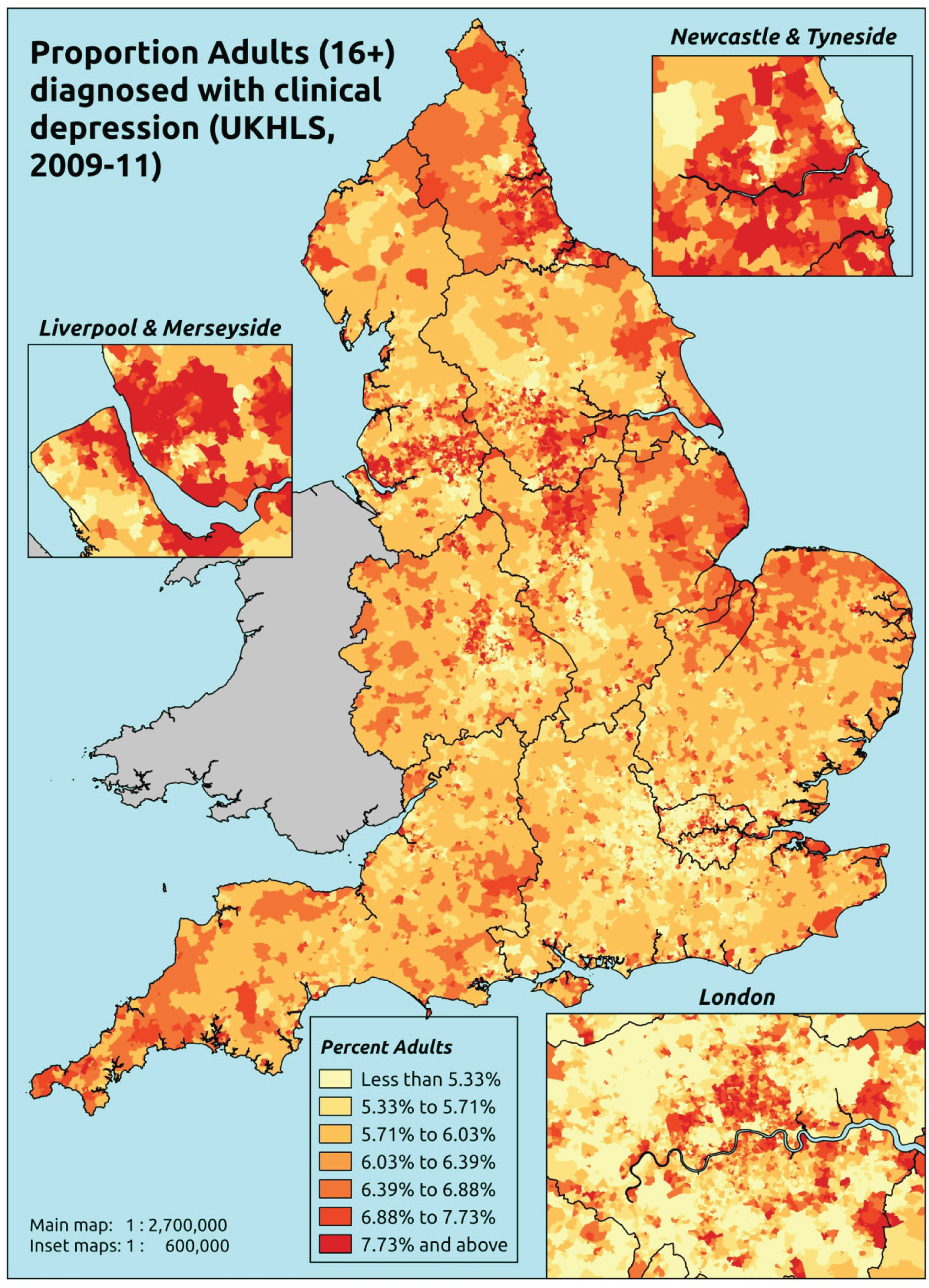
Response variable definition, provenance and prediction
Based on the question ‘Has a doctor or other health professional ever told you that you have . . . clinical depression’, here we estimate of the proportion of people in each age–sex cohort, and overall for adults aged ≥ 16 years, who have ever had doctor diagnosed clinical depression. As this explicitly refers to a doctor diagnosis, this marker is vulnerable to any sociodemographic or geographic variations in access to, or uptake of, care. (A smaller, but more recent, data set provides the basis for an alternative measure of the prevalence of adults who have ‘ever been diagnosed with clinical depression’ – see below).
The first wave of the UKHLS data set (n = 50,994) runs from January 2009 to January 2011 and includes multiple household respondents aged ≥ 16 from across the UK. The analytical data set is drawn from a subset of respondents living in England for whom data is available across all model response and predictor variables, namely whether or not told by a doctor they have clinical depression, along with information on age band, sex, ethnicity, LLTI, tenure and the IMD score of the LSOA of residence (n = 39,754). A single randomly selected adult is then drawn from each household, resulting in an analytical data set of 24,889 adults aged ≥ 16 years.
| Age band (years) | Females | Age band (years) | Males | ||||
|---|---|---|---|---|---|---|---|
| Does not have condition | Has condition | % | Does not have condition | Has condition | % | ||
| 16–24 | 1373 | 88 | 6.0 | 16–24 | 1095 | 27 | 2.4 |
| 25–34 | 2507 | 185 | 6.9 | 25–34 | 1673 | 70 | 4.0 |
| 35–49 | 3768 | 476 | 11.2 | 35–49 | 2843 | 187 | 6.2 |
| 50–64 | 2838 | 357 | 11.2 | 50–64 | 2201 | 201 | 8.4 |
| 65–74 | 1462 | 85 | 5.5 | 65–74 | 1196 | 62 | 4.9 |
| 75–84 | 938 | 33 | 3.4 | 75–84 | 716 | 19 | 2.6 |
| ≥ 85 | 304 | 10 | 3.2 | ≥ 85 | 174 | 1 | 0.6 |
| Females | 13,190 | 1234 | 8.6 | Males | 9898 | 567 | 5.4 |
| Total (males and females) | 23,088 | 1801 | 7.2 | ||||
Model parameters are applied to microsimulated LSOA-level census data to produce estimates of the number (and proportion) of people expected to ever have had doctor-diagnosed clinical depression in each age–sex cohort (and overall) in each of the 32,844 English LSOAs. As discussed in the report, bootstrapping is used to derive 95% CIs for the estimates. These LSOA-level prevalence rate estimates (and 95% CIs) are aggregated into a number of higher geographies, namely MSOAs, LAs, CCGs and regions (GORs). Proportionate attribution is used to restructure the prevalence rate estimates to align with 2001 MSOAs, as well as GP practice populations as defined by the 2011 NHS ADS.
Table 191 summarises how expected prevalence rates vary by age, sex and local deprivation (as measured by the 2010 IMD). There are 6569 LSOAs (with 9,226,227 adults) classified as being in the least deprived quintile; 6568 LSOAs (9,525,344 adults) in the second least deprived quintile; 6568 LSOAs (9,658,444 adults) in the third least deprived quintile; 6568 LSOAs (9,650,576 adults) in the fourth least deprived quintile; and 6568 LSOAs (9,535,167 adults) in the most deprived quintile. Note that, as a general rule, variations in prevalence rates reflect variations in the socioeconomic composition of populations in the different types of LSOA rather than variations in deprivation per se.
| Cohort | Least deprived quintile LSOAs | Second least deprived quintile LSOAs | Third least deprived quintile LSOAs | Fourth least deprived quintile LSOAs | Most deprived quintile LSOAs | All England |
|---|---|---|---|---|---|---|
| Female 16–24 | 4.8 (3.7 to 6.1) | 5.0 (4.0 to 6.2) | 5.2 (4.2 to 6.3) | 5.5 (4.4 to 6.4) | 6.1 (5.0 to 7.1) | 5.4 (4.3 to 6.5) |
| Female 25–34 | 5.8 (5.0 to 6.6) | 6.0 (5.3 to 6.9) | 6.3 (5.5 to 7.1) | 6.7 (5.9 to 7.5) | 7.5 (6.7 to 8.5) | 6.6 (5.8 to 7.4) |
| Female 35–49 | 8.9 (8.2 to 9.9) | 9.7 (8.8 to 10.6) | 10.4 (9.5 to 11.4) | 11.6 (10.7 to 12.5) | 13.7 (12.4 to 14.7) | 10.8 (9.9 to 11.8) |
| Female 50–64 | 9.4 (8.3 to 10.1) | 9.9 (9.0 to 10.7) | 10.6 (9.6 to 11.4) | 11.4 (10.3 to 12.4) | 13.0 (11.8 to 14.2) | 10.8 (9.7 to 11.6) |
| Female 65–74 | 5.1 (4.2 to 5.9) | 5.1 (4.2 to 6.0) | 5.1 (4.3 to 6.1) | 5.3 (4.3 to 6.3) | 5.6 (4.5 to 6.8) | 5.2 (4.3 to 6.2) |
| Female ≥ 75 | 2.9 (2.3 to 3.9) | 3.0 (2.4 to 4.0) | 3.2 (2.4 to 4.2) | 3.4 (2.6 to 4.5) | 3.7 (2.8 to 5.0) | 3.2 (2.5 to 4.3) |
| Females | 6.9 (6.1 to 7.8) | 7.2 (6.4 to 8.2) | 7.6 (6.7 to 8.5) | 8.2 (7.2 to 9.1) | 9.3 (8.2 to 10.4) | 7.9 (7.0 to 8.8) |
| Male 16–24 | 1.9 (1.4 to 2.6) | 2.0 (1.5 to 2.7) | 2.1 (1.5 to 2.7) | 2.3 (1.6 to 2.9) | 2.6 (1.8 to 3.3) | 2.2 (1.6 to 2.9) |
| Male 25–34 | 3.1 (2.4 to 3.7) | 3.3 (2.5 to 3.9) | 3.4 (2.6 to 4.1) | 3.7 (2.9 to 4.4) | 4.4 (3.5 to 5.2) | 3.7 (2.9 to 4.3) |
| Male 35–49 | 4.2 (3.7 to 4.8) | 4.7 (4.2 to 5.4) | 5.2 (4.7 to 6.0) | 6.1 (5.5 to 7.0) | 7.8 (6.9 to 8.8) | 5.6 (5.0 to 6.4) |
| Male 50–64 | 6.2 (5.5 to 6.8) | 6.8 (6.1 to 7.4) | 7.6 (6.7 to 8.2) | 8.5 (7.6 to 9.4) | 10.2 (9.2 to 11.4) | 7.8 (7.0 to 8.5) |
| Male 65–74 | 4.5 (3.5 to 5.5) | 4.8 (3.6 to 5.8) | 4.9 (3.8 to 6.0) | 5.2 (4.0 to 6.4) | 5.7 (4.4 to 7.0) | 5.0 (3.8 to 6.0) |
| Male ≥ 75 | 2.0 (1.4 to 2.9) | 2.1 (1.5 to 3.0) | 2.2 (1.5 to 3.1) | 2.3 (1.6 to 3.2) | 2.6 (1.8 to 3.5) | 2.2 (1.5 to 3.1) |
| Males | 4.1 (3.4 to 4.8) | 4.4 (3.7 to 5.2) | 4.7 (4.0 to 5.5) | 5.2 (4.4 to 6.0) | 6.2 (5.3 to 7.2) | 4.9 (4.2 to 5.7) |
| All | 5.6 (5.2 to 5.9) | 5.9 (5.5 to 6.2) | 6.2 (5.8 to 6.6) | 6.7 (6.3 to 7.1) | 7.8 (7.3 to 8.3) | 6.4 (6.1 to 6.8) |
| Factor (reference group) | Model coefficients | 95% CI | ||
|---|---|---|---|---|
| Estimate | SE | 2.5% CI | 97.50% | |
| (Intercept) | –3.27051 | 0.22045 | –3.70259 | –2.83844 |
| Age (16–24 years) | ||||
| 25–34 years | 0.14429 | 0.25224 | –0.35010 | 0.63869 |
| 35–49 years | 0.53848 | 0.22599 | 0.09554 | 0.98142 |
| 50–64 years | 0.62174 | 0.22917 | 0.17256 | 1.07092 |
| 65–74 years | 0.11690 | 0.26511 | –0.40271 | 0.63652 |
| 75–84 years | –0.69504 | 0.37895 | –1.43778 | 0.04771 |
| ≥ 85 years | –1.83787 | 1.08818 | –3.97070 | 0.29495 |
| Sex (females) | ||||
| Males | –1.11855 | 0.24067 | –1.59027 | –0.64682 |
| Ethnicity (white) | ||||
| Mixed | –0.43799 | 0.27041 | –0.96799 | 0.09201 |
| Black | –1.01326 | 0.16916 | –1.34481 | –0.68171 |
| Asian | –1.64876 | 0.23891 | –2.11703 | –1.18050 |
| Other | –1.56966 | 0.45377 | –2.45904 | –0.68027 |
| LLTI (no LTTI) | ||||
| LLTI | 1.33919 | 0.23349 | 0.88155 | 1.79683 |
| Tenure (owner–occupier) | ||||
| Social rent | 1.02122 | 0.25201 | 0.52727 | 1.51517 |
| Private rent or other tenure | 0.35313 | 0.26971 | –0.17550 | 0.88176 |
| LSOA deprivation score | ||||
| IMD score | –0.00227 | 0.00258 | –0.00733 | 0.00279 |
| Interaction effects | ||||
| 25–34 years and LLTI | 0.00648 | 0.25599 | –0.49525 | 0.50822 |
| 35–49 years and LLTI | –0.03076 | 0.23103 | –0.48357 | 0.42205 |
| 50–64 years and LLTI | –0.42518 | 0.23562 | –0.88701 | 0.03664 |
| 65–74 years and LLTI | –0.81919 | 0.28124 | –1.37043 | –0.26796 |
| 75–84 years and LLTI | –0.85097 | 0.39051 | –1.61637 | –0.08558 |
| ≥ 85 years and LLTI | 0.06041 | 1.07803 | –2.05253 | 2.17335 |
| Male and LLTI | 0.48401 | 0.11580 | 0.25705 | 0.71097 |
| Mixed and LLTI | 0.49348 | 0.35573 | –0.20374 | 1.19071 |
| Black and LLTI | 0.50986 | 0.21994 | 0.07877 | 0.94095 |
| Asian and LLTI | 0.48037 | 0.30365 | –0.11479 | 1.07552 |
| Other and LLTI | 0.91174 | 0.53938 | –0.14543 | 1.96892 |
| LLTI by LSOA IMD score | 0.01040 | 0.00326 | 0.00402 | 0.01678 |
| 25–34 years and social rent | –0.03381 | 0.30079 | –0.62336 | 0.55573 |
| 35–49 years and social rent | –0.01540 | 0.26980 | –0.54420 | 0.51340 |
| 50–64 years and social rent | –0.47440 | 0.27367 | –1.01079 | 0.06199 |
| 65–74 years and social rent | –0.80588 | 0.32183 | –1.43665 | –0.17510 |
| 75–84 years and social rent | –0.27175 | 0.38930 | –1.03478 | 0.49128 |
| ≥ 85 years and social rent | –0.11621 | 0.70722 | –1.50237 | 1.26995 |
| 25–34 years and private rent or other tenure | 0.18649 | 0.31919 | –0.43912 | 0.81211 |
| 35–49 years and private rent or other tenure | 0.31695 | 0.29545 | –0.26212 | 0.89603 |
| 50–64 years and private rent or other tenure | 0.13599 | 0.31079 | –0.47316 | 0.74515 |
| 65–74 years and private rent or other tenure | –0.94607 | 0.58533 | –2.09332 | 0.20118 |
| 75–84 years and private rent or other tenure | –0.19357 | 0.79074 | –1.74342 | 1.35627 |
| ≥ 85 years and private rent or other tenure | 0.43774 | 1.17569 | –1.86662 | 2.74209 |
| 25–34 years and male | 0.31776 | 0.28134 | –0.23366 | 0.86918 |
| 35–49 years and male | 0.16300 | 0.25534 | –0.33747 | 0.66347 |
| 50–64 years and male | 0.48776 | 0.25577 | –0.01355 | 0.98907 |
| 65–74 years and male | 0.74655 | 0.29378 | 0.17074 | 1.32236 |
| 75–84 years and male | 0.54506 | 0.37937 | –0.19851 | 1.28863 |
| ≥ 85 years and male | –0.85680 | 1.08710 | –2.98751 | 1.27391 |
FIGURE 169.
Parameter plots: diagnosed with clinical depression.
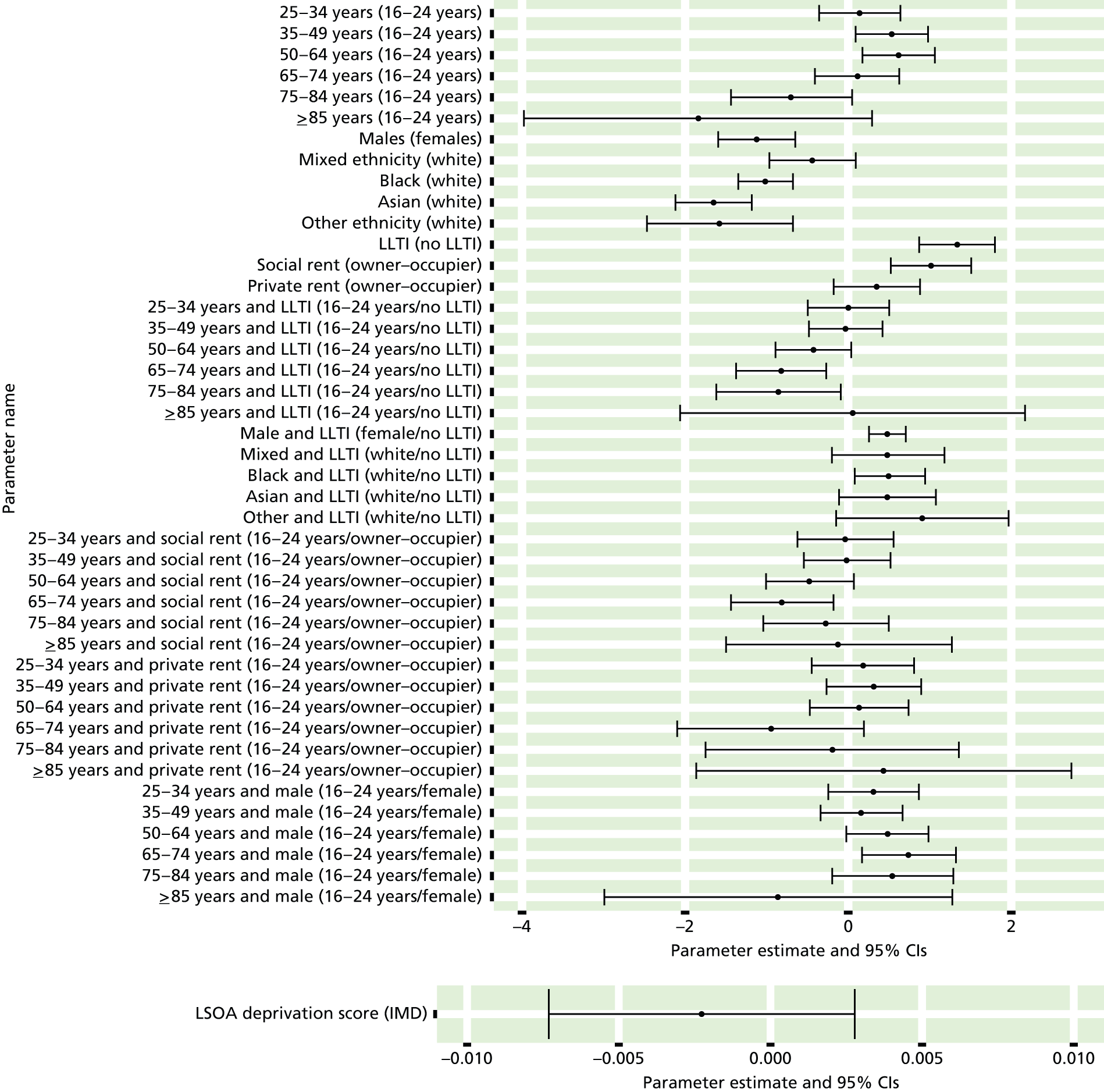
FIGURE 170.
Diagnosed with clinical depression: individual estimates and their 95% CIs. (a) MSOAs; (b) LAs; (c) CCGs; and (d) regions (GORs).
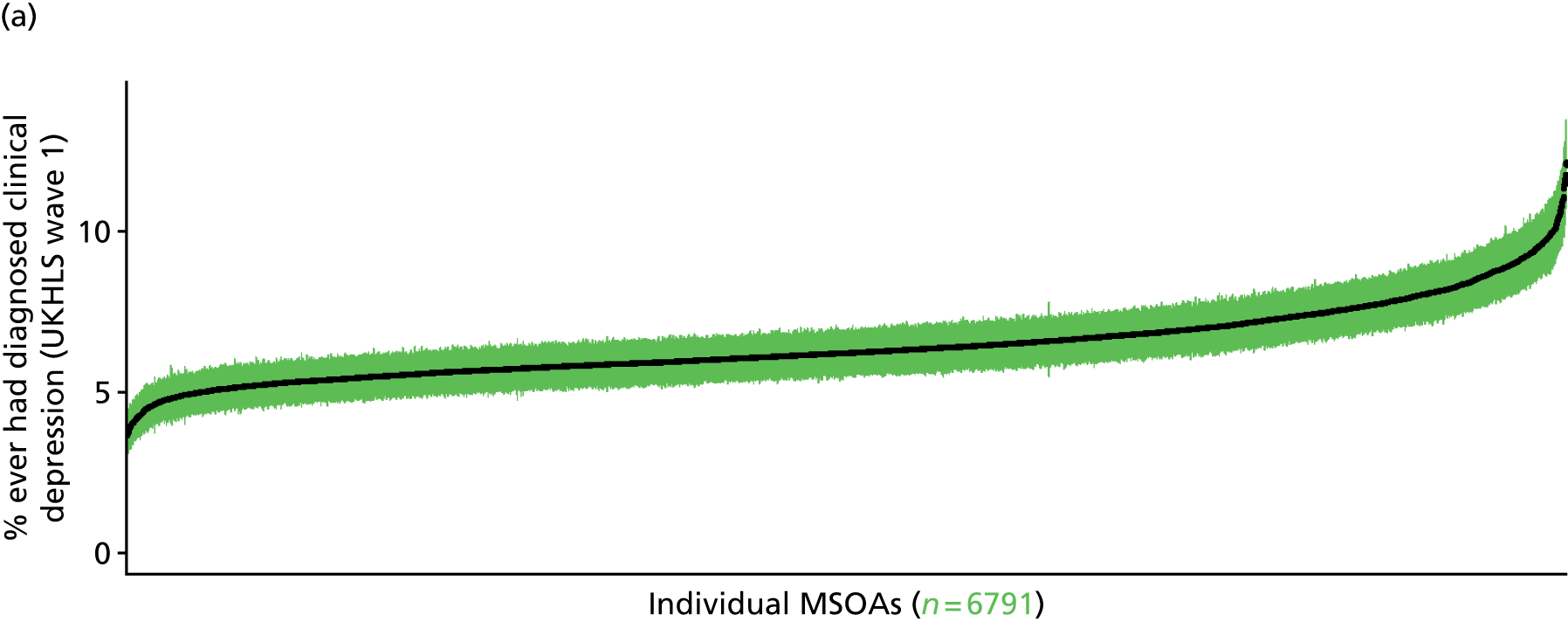


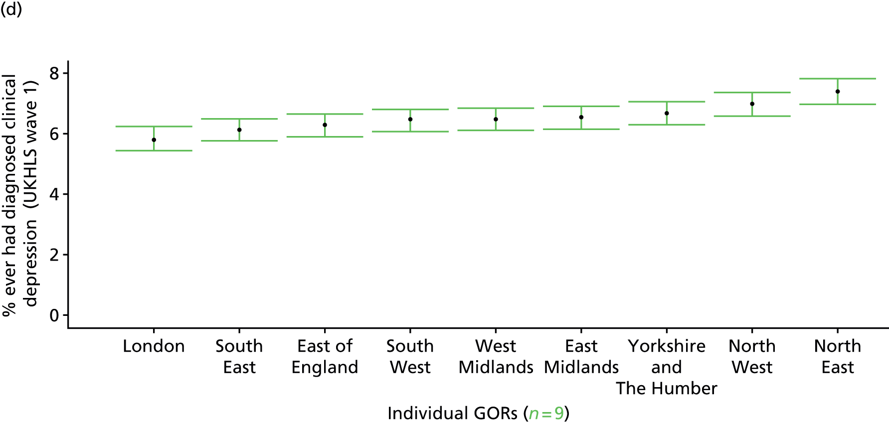
Current diagnosed clinical depression (UK Household Longitudinal Survey wave 1, 2009–11)
FIGURE 171.
Current diagnosed clinical depression: LSOA-level map. Contains Ordnance Survey data © Crown copyright and database right 2012.
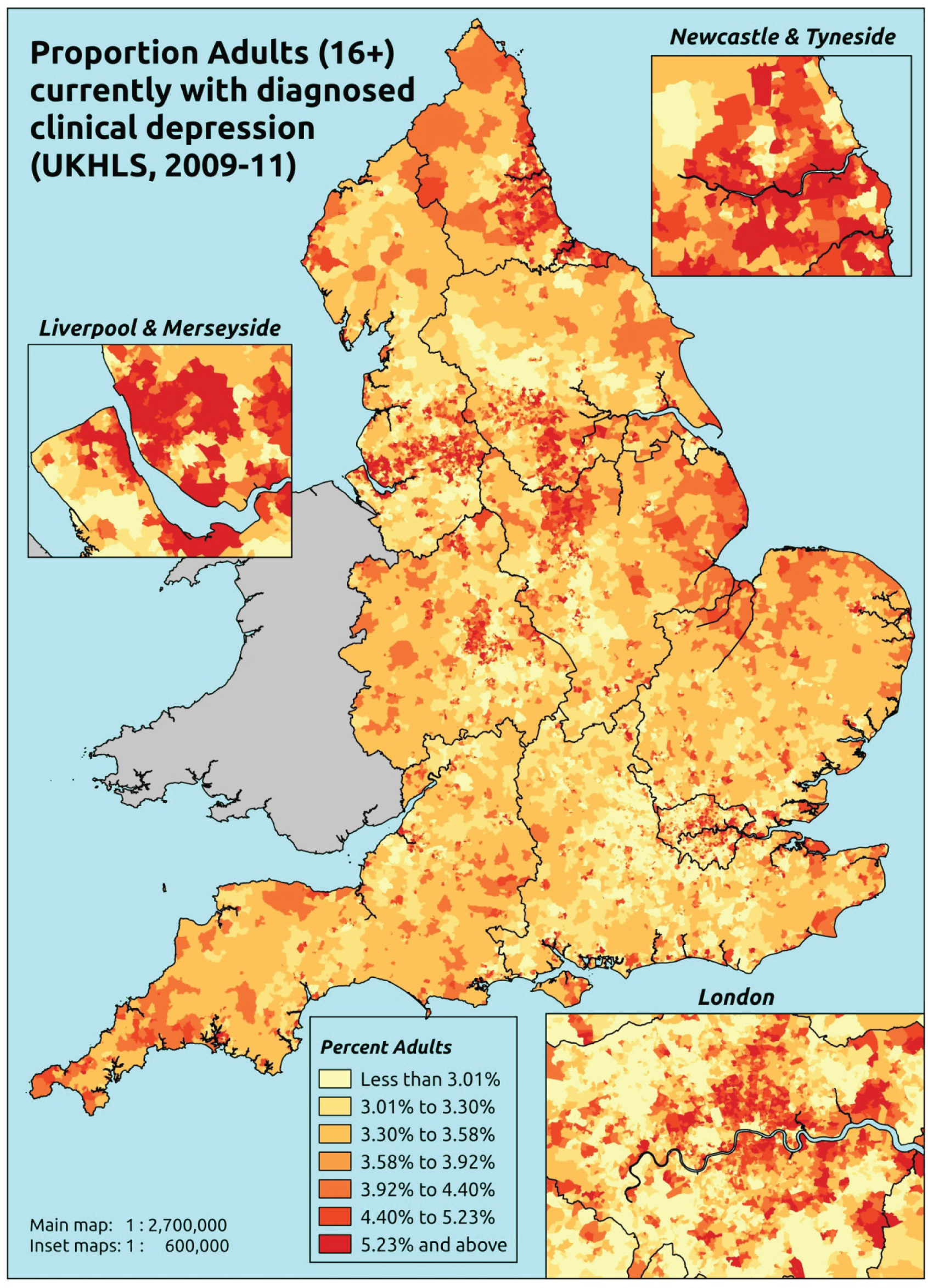
Response variable definition, provenance and prediction
Based on the question ‘Do you still have . . . clinical depression’, which is asked of respondents who answer yes to the question ‘Has a doctor or other health professional ever told you that you have . . . Clinical depression’, here we estimate of the proportion of people in each age–sex cohort, and overall for adults aged ≥ 16 years, who currently suffer from doctor-diagnosed clinical depression. As this explicitly refers to a doctor diagnosis, this marker is vulnerable to any sociodemographic or geographic variations in access to, or uptake of, care.
The first wave of the UKHLS data set (n = 50,994) runs from January 2009 to January 2011 and includes multiple household respondents aged ≥ 16 years from across the UK. The analytical data set is drawn from a subset of respondents living in England for whom data are available across all model response and predictor variables, namely whether or not they still have doctor-diagnosed clinical depression, along with information on age band, sex, ethnicity, LLTI, tenure and the IMD score of the LSOA of residence (n = 39,754). A single randomly selected adult is then drawn from each household, resulting in an analytical data set of 24,889 adults aged ≥ 16 years.
| Age band (years) | Females | Age band (years) | Males | ||||
|---|---|---|---|---|---|---|---|
| Does not have condition | Has condition | % | Does not have condition | Has condition | % | ||
| 16–24 | 1403 | 58 | 4.0 | 16–24 | 1100 | 22 | 2.0 |
| 25–34 | 2574 | 118 | 4.4 | 25–34 | 1693 | 50 | 2.9 |
| 35–49 | 3916 | 328 | 7.7 | 35–49 | 2888 | 142 | 4.7 |
| 50–64 | 2950 | 245 | 7.7 | 50–64 | 2254 | 148 | 6.2 |
| 65–74 | 1491 | 56 | 3.6 | 65–74 | 1216 | 42 | 3.3 |
| 75–84 | 943 | 28 | 2.9 | 75–84 | 720 | 15 | 2.0 |
| ≥ 85 | 307 | 7 | 2.2 | ≥ 85 | 175 | 0 | 0.0 |
| Females | 13,584 | 840 | 5.8 | Males | 10,046 | 419 | 4.0 |
| Adults | 23,630 | 1259 | 5.1 | ||||
Model parameters are applied to microsimulated LSOA-level census data to produce estimates of the number (and proportion) of people expected to currently suffer doctor-diagnosed clinical depression in each age–sex cohort (and overall) in each of the 32,844 English LSOAs. As discussed in the report, bootstrapping is used to derive 95% CIs for the estimates. These LSOA-level prevalence rate estimates (and 95% CIs) are aggregated into a number of higher geographies, namely MSOAs, LAs, CCGs and regions (GORs). Proportionate attribution is used to restructure the prevalence rate estimates to align with 2001 MSOAs, as well as GP practice populations as defined by the 2011 NHS ADS.
Table 194 summarises how expected prevalence rates vary by age, sex and local deprivation (as measured by the 2010 IMD). There are 6569 LSOAs (with 9,226,227 adults) classified as being in the least deprived quintile; 6568 LSOAs (9,525,344 adults) in the second least deprived quintile; 6568 LSOAs (9,658,444 adults) in the third least deprived quintile; 6568 LSOAs (9,650,576 adults) in the fourth least deprived quintile; and 6568 LSOAs (9,535,167 adults) in the most deprived quintile. Note that, as a general rule, variations in prevalence rates reflect variations in the socioeconomic composition of populations in the different types of LSOA rather than variations in deprivation per se.
| Cohort | Least deprived quintile LSOAs | Second least deprived quintile LSOAs | Third least deprived quintile LSOAs | Fourth least deprived quintile LSOAs | Most deprived quintile LSOAs | All England |
|---|---|---|---|---|---|---|
| Female 16–24 | 2.4 (2.0 to 3.0) | 2.6 (2.1 to 3.2) | 2.7 (2.2 to 3.4) | 3.0 (2.3 to 3.7) | 3.5 (2.7 to 4.1) | 2.9 (2.3 to 3.6) |
| Female 25–34 | 2.9 (2.4 to 3.4) | 3.1 (2.6 to 3.6) | 3.3 (2.8 to 3.8) | 3.7 (3.2 to 4.2) | 4.4 (3.8 to 5.1) | 3.6 (3.1 to 4.1) |
| Female 35–49 | 4.8 (4.3 to 5.3) | 5.3 (4.8 to 5.8) | 6.0 (5.4 to 6.5) | 7.0 (6.4 to 7.6) | 8.7 (8.0 to 9.6) | 6.4 (5.8 to 6.9) |
| Female 50–64 | 5.1 (4.5 to 5.8) | 5.7 (5.0 to 6.5) | 6.4 (5.7 to 7.2) | 7.6 (6.7 to 8.4) | 9.8 (8.6 to 10.8) | 6.8 (6.0 to 7.6) |
| Female 65–74 | 3.1 (2.8 to 3.9) | 3.4 (3.0 to 4.2) | 3.7 (3.3 to 4.6) | 4.3 (3.7 to 5.2) | 5.2 (4.4 to 6.4) | 3.8 (3.4 to 4.7) |
| Female ≥ 75 | 2.0 (1.5 to 2.6) | 2.1 (1.6 to 2.7) | 2.2 (1.8 to 2.9) | 2.5 (2.0 to 3.2) | 2.9 (2.3 to 3.8) | 2.3 (1.8 to 3.0) |
| Females | 3.8 (3.3 to 4.4) | 4.1 (3.6 to 4.8) | 4.5 (3.9 to 5.2) | 5.1 (4.5 to 5.8) | 6.3 (5.5 to 7.2) | 4.8 (4.2 to 5.5) |
| Male 16–24 | 1.4 (1.1 to 1.7) | 1.5 (1.2 to 1.8) | 1.6 (1.3 to 1.9) | 1.7 (1.4 to 2.1) | 2.1 (1.7 to 2.5) | 1.7 (1.3 to 2.0) |
| Male 25–34 | 1.7 (1.4 to 1.9) | 1.8 (1.6 to 2.1) | 2.0 (1.7 to 2.3) | 2.2 (1.9 to 2.6) | 2.9 (2.4 to 3.3) | 2.2 (1.9 to 2.5) |
| Male 35–49 | 2.7 (2.4 to 3.0) | 3.2 (2.8 to 3.5) | 3.7 (3.3 to 4.1) | 4.5 (4.1 to 5.0) | 6.1 (5.4 to 6.8) | 4.0 (3.7 to 4.5) |
| Male 50–64 | 3.1 (2.8 to 3.6) | 3.7 (3.2 to 4.2) | 4.3 (3.7 to 4.8) | 5.2 (4.6 to 6.1) | 7.2 (6.2 to 8.3) | 4.6 (4.0 to 5.2) |
| Male 65–74 | 2.1 (1.7 to 2.6) | 2.3 (2.0 to 2.9) | 2.6 (2.2 to 3.2) | 3.0 (2.6 to 3.8) | 3.8 (3.2 to 4.9) | 2.7 (2.3 to 3.4) |
| Male ≥ 75 | 1.5 (1.1 to 1.9) | 1.6 (1.2 to 2.0) | 1.7 (1.3 to 2.2) | 1.9 (1.5 to 2.5) | 2.3 (1.8 to 3.0) | 1.8 (1.4 to 2.3) |
| Males | 2.3 (2.0 to 2.7) | 2.6 (2.3 to 3.1) | 2.9 (2.5 to 3.4) | 3.4 (3.0 to 4.0) | 4.5 (3.9 to 5.2) | 3.2 (2.8 to 3.7) |
| All | 3.1 (2.9 to 3.4) | 3.4 (3.1 to 3.7) | 3.8 (3.5 to 4.0) | 4.3 (4.0 to 4.6) | 5.4 (5.0 to 5.9) | 4.0 (3.7 to 4.3) |
| Factor (reference group) | Model coefficients | 95% CI | ||
|---|---|---|---|---|
| Estimate | SE | 2.5% CI | 97.50% | |
| (Intercept) | –4.14813 | 0.19200 | –4.52445 | –3.77181 |
| Age (16–24 years) | ||||
| 25–34 years | 0.04213 | 0.19315 | –0.33645 | 0.42071 |
| 35–49 years | 0.52827 | 0.17604 | 0.18323 | 0.87330 |
| 50–64 years | 0.47360 | 0.19216 | 0.09696 | 0.85024 |
| 65–74 years | 0.03992 | 0.25408 | –0.45808 | 0.53792 |
| 75–84 years | –0.51029 | 0.38975 | –1.27420 | 0.25362 |
| ≥ 85 years | –1.31535 | 1.01575 | –3.30623 | 0.67553 |
| Sex (females) | ||||
| Males | –0.75317 | 0.11797 | –0.98440 | –0.52195 |
| Ethnicity (white) | ||||
| Mixed | –0.12747 | 0.19711 | –0.51380 | 0.25886 |
| Black | –0.54765 | 0.11947 | –0.78180 | –0.31349 |
| Asian | –1.26095 | 0.16566 | –1.58564 | –0.93626 |
| Other | –0.78907 | 0.25991 | –1.29849 | –0.27965 |
| LLTI (no LTTI) | ||||
| LLTI | 1.52111 | 0.26927 | 0.99335 | 2.04888 |
| Tenure (owner–occupier) | ||||
| Social rent | 1.22029 | 0.14189 | 0.94219 | 1.49838 |
| Private rent or other tenure | 0.52233 | 0.16543 | 0.19809 | 0.84658 |
| LSOA deprivation score | ||||
| IMD score | 0.00375 | 0.00403 | –0.00414 | 0.01165 |
| Interaction effects | ||||
| Male and LLTI | 0.50620 | 0.14211 | 0.22767 | 0.78474 |
| 25–34 years and LLTI | 0.35113 | 0.29116 | –0.21954 | 0.92179 |
| 35–49 years and LLTI | 0.19088 | 0.26218 | –0.32298 | 0.70475 |
| 50–64 years and LLTI | –0.11726 | 0.27212 | –0.65061 | 0.41609 |
| 65–74 years and LLTI | –0.69747 | 0.33561 | –1.35526 | –0.03969 |
| 75–84 years and LLTI | –0.67117 | 0.46375 | –1.58013 | 0.23779 |
| ≥ 85 years and LLTI | –0.68891 | 1.11189 | –2.86821 | 1.49039 |
| LLTI by LSOA IMD score | 0.01047 | 0.00385 | 0.00292 | 0.01802 |
| Social rent by LSOA IMD score | –0.00725 | 0.00429 | –0.01567 | 0.00117 |
| Private rent or other tenure by LSOA IMD score | 0.00476 | 0.00542 | –0.00587 | 0.01539 |
FIGURE 172.
Parameter plots: current diagnosed clinical depression.

FIGURE 173.
Current diagnosed clinical depression: individual estimates and their 95% CIs. (a) MSOAs; (b) LAs; (c) CCGs; and (d) regions (GORs).
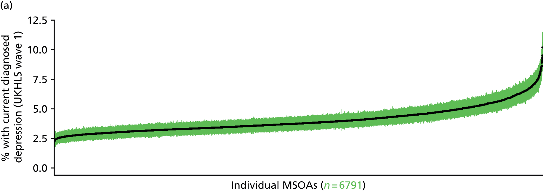
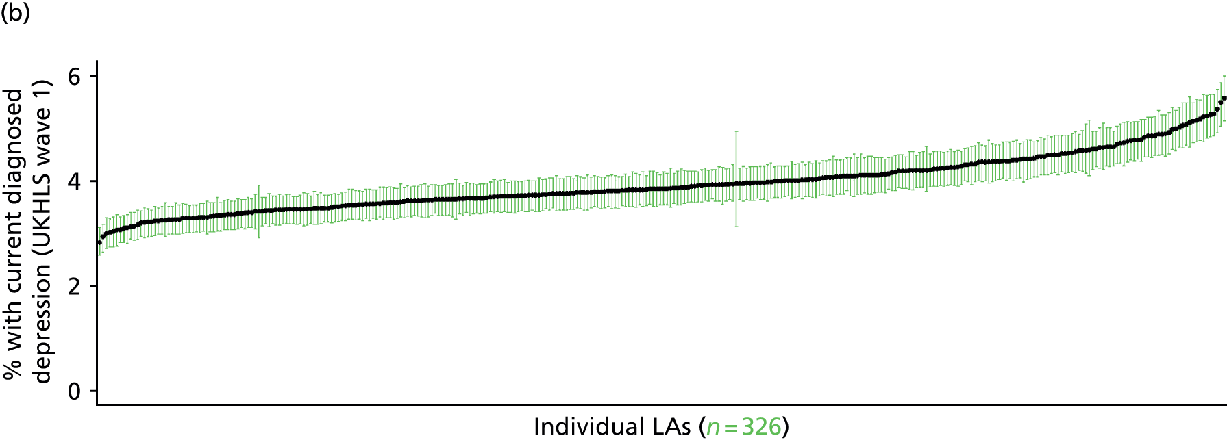
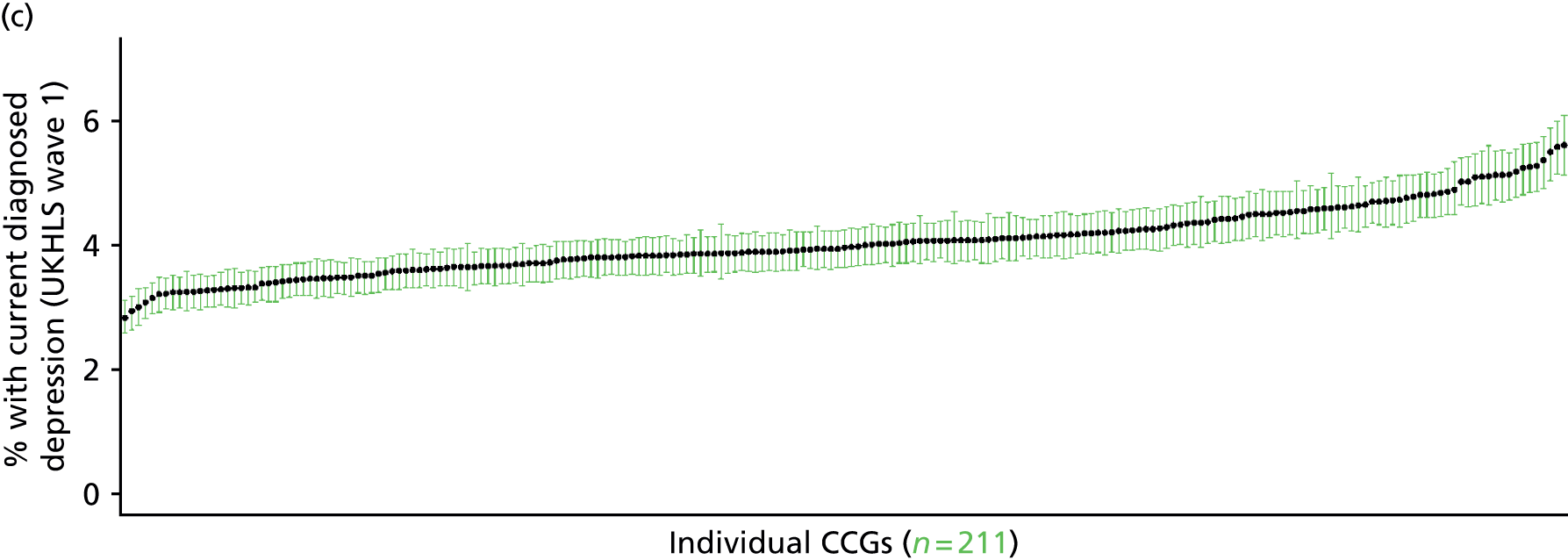
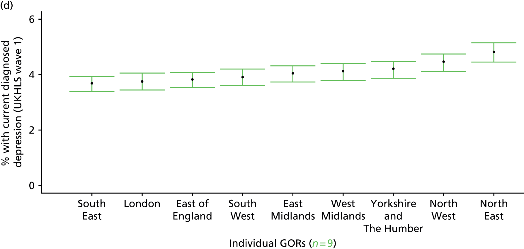
Ever been diagnosed with clinical depression (UK Household Longitudinal Survey, waves 1 and 2)
FIGURE 174.
Ever been diagnosed with clinical depression: LSOA-level map. Contains Ordnance Survey data © Crown copyright and database right 2012.

Response variable definition, provenance and prediction
This concerns respondents who appear in both waves of the UKHLS and is based on the second wave question ‘Have you been diagnosed with clinical depression since your last interview’, and the first wave question ‘Has a doctor or other health professional ever told you that you have . . . clinical depression ‘. Taken together, this describes whether or not people in wave 2 (who were also in wave 1) have ever been diagnosed with clinical depression. As such, it represents a more recent estimate of the prevalence of doctor-diagnosed clinical depression, although the size of the sample (n = 8434) is somewhat smaller than that based on wave 1 respondents (n = 24,899). As this explicitly refers to a doctor diagnosis, this marker is vulnerable to any sociodemographic or geographic variations in access to, or uptake of, care.
The first wave of the UKHLS data set (n = 50,994) runs from January 2009 to January 2011 and includes multiple household respondents aged ≥ 16 years from across the UK. The second wave (n = 31,242) runs from January 2010 to January 2012 and similarly comprises multiple household respondents aged ≥ 16 years from across the UK. Here the analytical data set is drawn from the subset of second wave respondents living in England who were also interviewed during the first wave and for whom data is available across all model response and predictor variables, namely that they reported (in the first wave questionnaire) whether they had ever been doctor-diagnosed with clinical depression, that they reported (in the second wave questionnaire) whether or not they had been diagnosed with clinical depression since their last interview, along with information on age band, sex, ethnicity, LLTI, tenure and the IMD score of the LSOA of residence (n = 12,756). A single randomly selected adult is then drawn from each household, resulting in an analytical data set of 8434 adults aged ≥ 16 years.
| Age band (years) | Females | Age band (years) | Males | ||||
|---|---|---|---|---|---|---|---|
| Does not have condition | Has condition | % | Does not have condition | Has condition | % | ||
| 16–24 | 305 | 27 | 8.1 | 16–24 | 240 | 9 | 3.6 |
| 25–34 | 731 | 70 | 8.7 | 25–34 | 440 | 22 | 4.8 |
| 35–49 | 1310 | 167 | 11.3 | 35–49 | 838 | 63 | 7.0 |
| 50–64 | 1126 | 152 | 11.9 | 50–64 | 821 | 74 | 8.3 |
| 65–74 | 591 | 48 | 7.5 | 65–74 | 488 | 27 | 5.2 |
| 75–84 | 396 | 17 | 4.1 | 75–84 | 259 | 12 | 4.4 |
| ≥ 85 | 114 | 4 | 3.4 | ≥ 85 | 82 | 1 | 1.2 |
| Females | 4573 | 485 | 9.6 | Males | 3168 | 208 | 6.2 |
| Total (males and females) | 7741 | 693 | 8.2 | ||||
Model parameters are applied to microsimulated LSOA-level census data to produce estimates of the number (and proportion) of people expected ever to have been diagnosed with clinical depression in each age–sex cohort (and overall) in each of the 32,844 English LSOAs. As discussed in the report, bootstrapping is used to derive 95% CIs for the estimates. These LSOA-level prevalence rate estimates (and 95% CIs) are aggregated into a number of higher geographies, namely MSOAs, LAs, CCGs and regions (GORs). Proportionate attribution is used to restructure the prevalence rate estimates to align with 2001 MSOAs, as well as GP practice populations as defined by the 2011 NHS ADS.
Table 197 summarises how expected prevalence rates vary by age, sex and local deprivation (as measured by the 2010 IMD). There are 6569 LSOAs (with 9,226,227 adults) classified as being in the least deprived quintile; 6568 LSOAs (9,525,344 adults) in the second least deprived quintile; 6568 LSOAs (9,658,444 adults) in the third least deprived quintile; 6568 LSOAs (9,650,576 adults) in the fourth least deprived quintile; and 6568 LSOAs (9,535,167 adults) in the most deprived quintile. Note that, as a general rule, variations in prevalence rates reflect variations in the socioeconomic composition of populations in the different types of LSOA rather than variations in deprivation per se.
| Cohort | Least deprived quintile LSOAs | Second least deprived quintile LSOAs | Third least deprived quintile LSOAs | Fourth least deprived quintile LSOAs | Most deprived quintile LSOAs | All England |
|---|---|---|---|---|---|---|
| Female 16–24 | 5.9 (4.4 to 7.6) | 6.1 (4.5 to 7.9) | 6.3 (4.7 to 8.2) | 6.6 (4.9 to 8.6) | 7.2 (5.4 to 9.3) | 6.5 (4.8 to 8.4) |
| Female 25–34 | 6.8 (5.5 to 8.1) | 7.0 (5.6 to 8.4) | 7.2 (5.8 to 8.6) | 7.5 (6.0 to 9.0) | 8.3 (6.6 to 9.8) | 7.5 (6.0 to 8.9) |
| Female 35–49 | 8.9 (7.9 to 9.7) | 9.6 (8.4 to 10.4) | 10.4 (9.1 to 11.3) | 11.4 (10.0 to 12.6) | 13.2 (11.6 to 14.6) | 10.7 (9.4 to 11.7) |
| Female 50–64 | 10.0 (8.8 to 11.4) | 10.7 (9.5 to 12.2) | 11.5 (10.1 to 13.0) | 12.8 (11.2 to 14.5) | 14.8 (12.9 to 17.0) | 11.8 (10.4 to 13.4) |
| Female 65–74 | 7.1 (5.7 to 8.5) | 7.4 (5.9 to 8.9) | 7.9 (6.2 to 9.3) | 8.3 (6.7 to 9.9) | 9.3 (7.3 to 11.1) | 7.9 (6.3 to 9.4) |
| Female ≥ 75 | 4.1 (2.8 to 5.3) | 4.2 (2.9 to 5.4) | 4.4 (3.0 to 5.6) | 4.7 (3.1 to 5.9) | 5.1 (3.4 to 6.6) | 4.5 (3.0 to 5.7) |
| Females | 7.7 (6.5 to 9.0) | 8.1 (6.8 to 9.4) | 8.6 (7.1 to 9.9) | 9.2 (7.6 to 10.7) | 10.4 (8.6 to 12.1) | 8.8 (7.4 to 10.2) |
| Male 16–24 | 3.6 (2.6 to 4.9) | 3.8 (2.7 to 5.1) | 4.0 (2.9 to 5.3) | 4.2 (3.0 to 5.6) | 4.7 (3.4 to 6.4) | 4.1 (3.0 to 5.5) |
| Male 25–34 | 4.0 (3.0 to 4.8) | 4.1 (3.2 to 5.0) | 4.2 (3.3 to 5.1) | 4.5 (3.5 to 5.5) | 5.1 (3.9 to 6.2) | 4.5 (3.5 to 5.4) |
| Male 35–49 | 5.3 (4.4 to 6.0) | 5.8 (4.9 to 6.6) | 6.4 (5.4 to 7.3) | 7.3 (6.2 to 8.4) | 8.9 (7.6 to 10.4) | 6.7 (5.7 to 7.8) |
| Male 50–64 | 6.1 (5.1 to 7.2) | 6.8 (5.7 to 7.9) | 7.4 (6.2 to 8.8) | 8.5 (7.1 to 10.0) | 10.4 (8.5 to 12.4) | 7.7 (6.4 to 9.1) |
| Male 65–74 | 4.5 (3.6 to 5.7) | 4.8 (3.8 to 6.1) | 5.2 (4.0 to 6.5) | 5.8 (4.4 to 7.1) | 6.6 (5.0 to 8.2) | 5.3 (4.1 to 6.6) |
| Male ≥ 75 | 2.8 (1.9 to 3.8) | 2.9 (2.0 to 4.0) | 3.1 (2.1 to 4.2) | 3.4 (2.2 to 4.5) | 3.6 (2.4 to 5.0) | 3.1 (2.1 to 4.2) |
| Males | 4.8 (3.9 to 5.8) | 5.1 (4.2 to 6.2) | 5.5 (4.4 to 6.6) | 6.1 (4.9 to 7.3) | 7.1 (5.7 to 8.7) | 5.7 (4.6 to 6.9) |
| All | 6.3 (5.8 to 6.9) | 6.7 (6.1 to 7.3) | 7.1 (6.4 to 7.7) | 7.7 (6.8 to 8.4) | 8.8 (7.8 to 9.8) | 7.3 (6.6 to 7.9) |
| Factor (reference group) | Model coefficients | 95% CI | ||
|---|---|---|---|---|
| Estimate | SE | 2.5% CI | 97.50% | |
| (Intercept) | –3.20525 | 0.22865 | –3.65341 | –2.75709 |
| Age (16–24 years) | ||||
| 25–34 years | 0.31673 | 0.24556 | –0.16458 | 0.79803 |
| 35–49 years | 0.47023 | 0.23336 | 0.01285 | 0.92762 |
| 50–64 years | 0.54806 | 0.23936 | 0.07891 | 1.01721 |
| 65–74 years | 0.21118 | 0.28107 | –0.33973 | 0.76208 |
| 75–84 years | –0.31178 | 0.40104 | –1.09781 | 0.47425 |
| ≥ 85 years | –1.35252 | 1.02813 | –3.36766 | 0.66262 |
| Sex (females) | ||||
| Males | –0.64438 | 0.12622 | –0.89176 | –0.39700 |
| Ethnicity (white) | ||||
| Mixed | 0.05616 | 0.38218 | –0.69292 | 0.80524 |
| Black | –0.45637 | 0.26057 | –0.96709 | 0.05436 |
| Asian | –1.02405 | 0.37418 | –1.75745 | –0.29065 |
| Other | –0.45364 | 0.44084 | –1.31769 | 0.41041 |
| LLTI (no LTTI) | ||||
| LLTI | 1.91352 | 0.40822 | 1.11341 | 2.71363 |
| Tenure (owner–occupier) | ||||
| Social rent | 0.69449 | 0.10721 | 0.48436 | 0.90463 |
| Private rent or other tenure | 0.40230 | 0.12501 | 0.15729 | 0.64731 |
| LSOA deprivation score | ||||
| IMD score | 0.00354 | 0.00278 | –0.00191 | 0.00899 |
| Interaction effects | ||||
| 25–34 years and LLTI | –0.78413 | 0.48006 | –1.72504 | 0.15678 |
| 35–49 years and LLTI | –0.42622 | 0.43106 | –1.27111 | 0.41867 |
| 50–64 years and LLTI | –0.84258 | 0.43040 | –1.68616 | 0.00100 |
| 65–74 years and LLTI | –1.30853 | 0.47215 | –2.23395 | –0.38311 |
| 75–84 years and LLTI | –1.42002 | 0.57611 | –2.54920 | –0.29084 |
| ≥ 85 years and LLTI | –0.90099 | 1.19819 | –3.24944 | 1.44745 |
| Male and LLTI | 0.31797 | 0.17921 | –0.03328 | 0.66922 |
FIGURE 175.
Parameter plots: ever been diagnosed with clinical depression.

FIGURE 176.
Ever been diagnosed with clinical depression: individual estimates and their 95% CIs. (a) MSOAs; (b) LAs; (c) CCGs; and (d) regions (GORs).
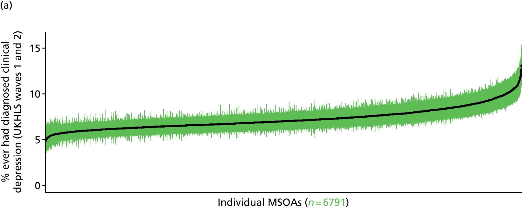
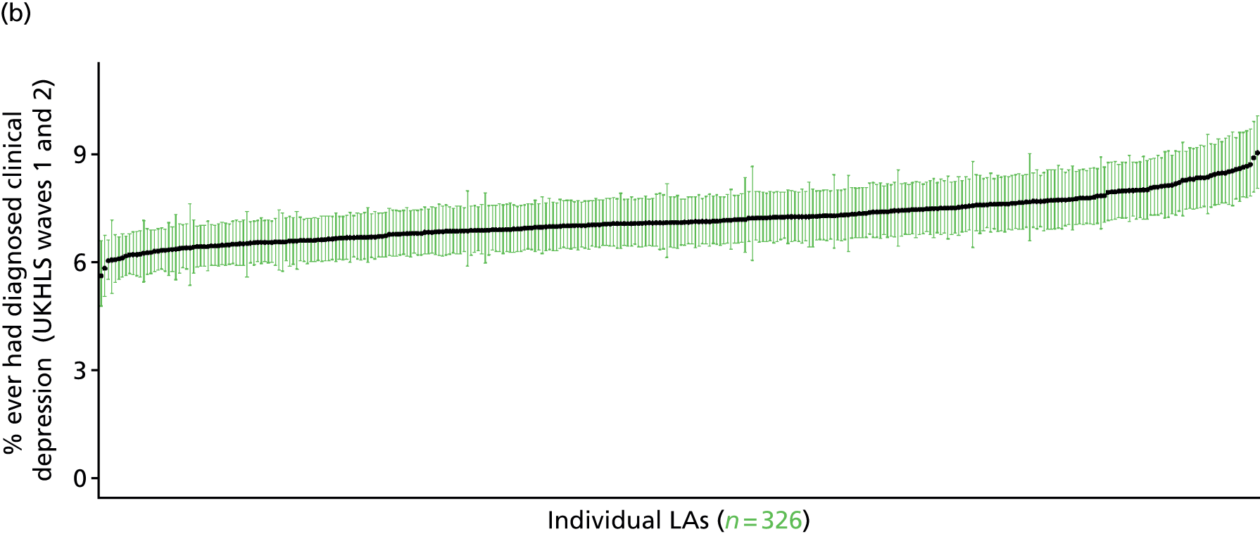
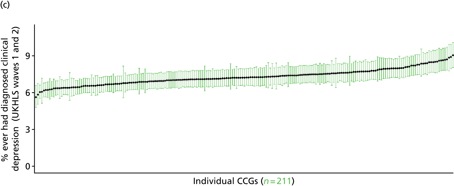

Incidence of diagnosis of clinical depression (UK Household Longitudinal Survey, waves 1 and 2)
FIGURE 177.
Incidence of diagnosis of clinical depression: LSOA-level map. Contains Ordnance Survey data © Crown copyright and database right 2012.

Response variable definition, provenance and prediction
Based on the question, ‘Have you been diagnosed with clinical depression since your last interview’, this provides an approximate estimate of the incidence of diagnosis of clinical depression. (People who were diagnosed with clinical depression prior to their first wave interview will answer ‘no’ to this question, so this cannot be used as a marker of the prevalence of clinical depression.) This is problematic as a measure of incidence, as the time interval (in months) between interviews varies, as illustrated below.
FIGURE 178.
Interval (in months) between UKHLS respondents’ wave 1 and 2 interviews (n = 11,448).
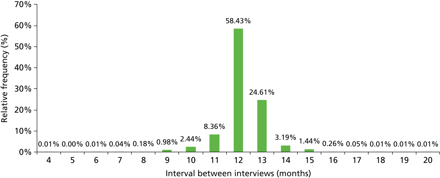
Nevertheless, with a mean interval of 12.2 months this should yield a reasonable estimate of the annual incidence of diagnosis of clinical depression during the period 2009–11. As this explicitly refers to a doctor diagnosis, this measure of incidence will reflect any sociodemographic or geographic variations in access to, or uptake of, care.
The first wave of the UKHLS data set (n = 50,994) runs from January 2009 to January 2011 and includes multiple household respondents aged ≥ 16 years from across the UK. The second wave (n = 31,242) runs from January 2010 to January 2012 and similarly comprises multiple household respondents aged ≥ 16 years from across the UK. Here the analytical data set is drawn from the subset of second wave respondents living in England who were also interviewed during the first wave and for whom data are available across all model response and predictor variables, namely that they reported (in the second wave questionnaire) whether or not they had been diagnosed with clinical depression since their last interview, along with information on age band, sex, ethnicity, LLTI, tenure and the IMD score of the LSOA of residence (n = 17,614). A single randomly selected adult is then drawn from each household, resulting in an analytical data set of 11,448 adults aged ≥ 16 years. (Note that in this instance we do not require a valid response to the first wave question about ever having been diagnosed with clinical depression.)
| Age band (years) | Females | Age band (years) | Males | ||||
|---|---|---|---|---|---|---|---|
| Does not have condition | Has condition | % | Does not have condition | Has condition | % | ||
| 16–24 | 449 | 17 | 3.6 | 16–24 | 338 | 5 | 1.5 |
| 25–34 | 1032 | 28 | 2.6 | 25–34 | 693 | 8 | 1.1 |
| 35–49 | 1894 | 52 | 2.7 | 35–49 | 1268 | 22 | 1.7 |
| 50–64 | 1662 | 38 | 2.2 | 50–64 | 1161 | 17 | 1.4 |
| 65–74 | 844 | 11 | 1.3 | 65–74 | 651 | 6 | 0.9 |
| 75–84 | 573 | 5 | 0.9 | 75–84 | 366 | 4 | 1.1 |
| ≥ 85 | 187 | 3 | 1.6 | ≥ 85 | 113 | 1 | 0.9 |
| Females | 6641 | 154 | 2.3 | Males | 4590 | 63 | 1.4 |
| Total (males and females) | 11,231 | 217 | 1.9 | ||||
Model parameters are applied to microsimulated LSOA-level census data to produce estimates of the number (and proportion) of people expected to be diagnosed with clinical depression during a 12-month period in each age–sex cohort (and overall) in each of the 32,844 English LSOAs. As discussed in the report, bootstrapping is used to derive 95% CIs for the estimates. These LSOA-level prevalence rate estimates (and 95% CIs) are aggregated into a number of higher geographies, namely MSOAs, LAs, CCGs and regions (GORs). Proportionate attribution is used to restructure the prevalence rate estimates to align with 2001 MSOAs, as well as GP practice populations as defined by the 2011 NHS ADS.
Table 200 summarises how expected prevalence rates vary by age, sex and local deprivation (as measured by the 2010 IMD). There are 6569 LSOAs (with 9,226,227 adults) classified as being in the least deprived quintile; 6568 LSOAs (9,525,344 adults) in the second least deprived quintile; 6568 LSOAs (9,658,444 adults) in the third least deprived quintile; 6568 LSOAs (9,650,576 adults) in the fourth least deprived quintile; and 6568 LSOAs (9,535,167 adults) in the most deprived quintile. Note that, as a general rule, variations in prevalence rates reflect variations in the socioeconomic composition of populations in the different types of LSOA rather than variations in deprivation per se.
| Cohort | Least deprived quintile LSOAs | Second least deprived quintile LSOAs | Third least deprived quintile LSOAs | Fourth least deprived quintile LSOAs | Most deprived quintile LSOAs | All England |
|---|---|---|---|---|---|---|
| Female 16–24 | 3.7 (1.9 to 5.6) | 3.8 (1.9 to 5.7) | 3.9 (2.0 to 5.8) | 4.2 (2.1 to 6.3) | 4.8 (2.4 to 7.1) | 4.1 (2.1 to 6.2) |
| Female 25–34 | 1.7 (1.0 to 2.7) | 1.8 (1.1 to 2.8) | 1.9 (1.1 to 2.8) | 2.0 (1.2 to 3.1) | 2.4 (1.4 to 3.7) | 2.0 (1.2 to 3.1) |
| Female 35–49 | 1.4 (1.1 to 1.9) | 1.5 (1.1 to 2.1) | 1.7 (1.3 to 2.3) | 2.0 (1.5 to 2.6) | 2.6 (1.9 to 3.4) | 1.9 (1.4 to 2.4) |
| Female 50–64 | 1.3 (0.9 to 1.8) | 1.4 (0.9 to 2.0) | 1.6 (1.0 to 2.2) | 1.9 (1.3 to 2.7) | 2.5 (1.7 to 3.6) | 1.7 (1.1 to 2.4) |
| Female 65–74 | 1.4 (0.8 to 2.2) | 1.5 (0.8 to 2.4) | 1.6 (1.0 to 2.6) | 2.0 (1.1 to 3.1) | 2.6 (1.4 to 4.1) | 1.8 (1.0 to 2.8) |
| Female ≥ 75 | 2.4 (1.1 to 4.0) | 2.5 (1.2 to 4.3) | 2.7 (1.3 to 4.6) | 3.0 (1.5 to 5.2) | 3.7 (1.9 to 6.5) | 2.8 (1.4 to 4.8) |
| Females | 1.8 (1.1 to 2.7) | 1.9 (1.1 to 2.9) | 2.1 (1.3 to 3.1) | 2.4 (1.5 to 3.6) | 3.0 (1.8 to 4.5) | 2.2 (1.4 to 3.3) |
| Male 16–24 | 3.2 (1.7 to 4.8) | 3.2 (1.7 to 4.8) | 3.4 (1.8 to 4.9) | 3.6 (2.0 to 5.4) | 4.2 (2.2 to 6.4) | 3.6 (1.9 to 5.2) |
| Male 25–34 | 1.4 (0.8 to 2.3) | 1.5 (0.9 to 2.3) | 1.6 (0.9 to 2.4) | 1.7 (0.9 to 2.6) | 2.0 (1.1 to 3.1) | 1.7 (0.9 to 2.6) |
| Male 35–49 | 1.2 (0.8 to 1.7) | 1.3 (0.8 to 1.9) | 1.4 (0.9 to 2.1) | 1.7 (1.1 to 2.5) | 2.1 (1.3 to 3.3) | 1.5 (1.0 to 2.3) |
| Male 50–64 | 1.1 (0.6 to 1.6) | 1.2 (0.7 to 1.8) | 1.3 (0.8 to 2.0) | 1.6 (1.0 to 2.4) | 2.1 (1.3 to 3.2) | 1.4 (0.9 to 2.2) |
| Male 65–74 | 1.2 (0.6 to 1.9) | 1.3 (0.6 to 2.1) | 1.4 (0.7 to 2.4) | 1.7 (0.8 to 2.9) | 2.2 (1.0 to 3.8) | 1.5 (0.7 to 2.6) |
| Male ≥ 75 | 2.1 (0.9 to 3.4) | 2.3 (1.0 to 3.6) | 2.4 (1.0 to 3.9) | 2.8 (1.2 to 4.6) | 3.3 (1.5 to 5.8) | 2.5 (1.1 to 4.1) |
| Males | 1.5 (0.8 to 2.3) | 1.6 (0.9 to 2.5) | 1.8 (1.0 to 2.7) | 2.0 (1.1 to 3.1) | 2.5 (1.4 to 4.0) | 1.9 (1.1 to 2.9) |
| All | 1.7 (1.4 to 2.0) | 1.8 (1.5 to 2.2) | 1.9 (1.6 to 2.4) | 2.2 (1.9 to 2.8) | 2.8 (2.2 to 3.5) | 2.1 (1.7 to 2.6) |
| Factor (reference group) | Model coefficients | 95% CI | ||
|---|---|---|---|---|
| Estimate | Standard error | 2.5% CI | 97.50% | |
| (Intercept) | –3.31248 | 0.43025 | –4.15577 | –2.46919 |
| Age (16–24 years) | ||||
| 25–34 years | –0.95707 | 0.51064 | –1.95793 | 0.04378 |
| 35–49 years | –1.30457 | 0.45263 | –2.19172 | –0.41742 |
| 50–64 years | –1.58920 | 0.47168 | –2.51368 | –0.66471 |
| 65–74 years | –1.58624 | 0.58216 | –2.72727 | –0.44521 |
| 75–84 years | 0.06859 | 0.77132 | –1.44319 | 1.58037 |
| ≥ 85 years | –2.71679 | 1.05476 | –4.78412 | –0.64946 |
| Sex (females) | ||||
| Males | –0.04736 | 0.26441 | –0.56560 | 0.47089 |
| Ethnicity (white) | ||||
| Mixed | –0.31139 | 0.72894 | –1.74011 | 1.11733 |
| Black | –0.87083 | 0.59020 | –2.02762 | 0.28597 |
| Asian | 0.38725 | 0.38460 | –0.36657 | 1.14108 |
| Other | –0.26081 | 0.73735 | –1.70602 | 1.18439 |
| LLTI (no LTTI) | ||||
| LLTI | 1.07034 | 0.21233 | 0.65418 | 1.4865 |
| Tenure (owner–occupier) | ||||
| Social rent | 0.86057 | 0.35043 | 0.17372 | 1.54742 |
| Private rent or other tenure | –0.67455 | 0.41468 | –1.48733 | 0.13823 |
| LSOA deprivation score | ||||
| IMD score | –0.01962 | 0.01727 | –0.05347 | 0.01423 |
| Interaction effects | ||||
| 25–34 years by LSOA IMD | 0.02603 | 0.01901 | –0.01124 | 0.06329 |
| 35–49 years by LSOA IMD | 0.03981 | 0.01707 | 0.00636 | 0.07326 |
| 50–64 years by LSOA IMD | 0.03760 | 0.01763 | 0.00304 | 0.07215 |
| 65–74 years by LSOA IMD | 0.01024 | 0.02357 | –0.03596 | 0.05644 |
| 75–84 years by LSOA IMD | –0.17262 | 0.07376 | –0.31718 | –0.02805 |
| ≥ 85 years by LSOA IMD | 0.04914 | 0.03488 | –0.01923 | 0.11750 |
| Social rent by LSOA IMD score | –0.00987 | 0.00994 | –0.02936 | 0.00962 |
| Private rent or other tenure by LSOA IMD score | 0.02522 | 0.01191 | 0.00188 | 0.04855 |
| LLTI and social rent | 0.33369 | 0.32954 | –0.31220 | 0.97959 |
| LLTI and private rent or other tenure | 0.93068 | 0.40569 | 0.13552 | 1.72583 |
| Male by LSOA IMD | –0.01837 | 0.00922 | –0.03644 | –0.00030 |
FIGURE 179.
Parameter plots: incidence of diagnosis of clinical depression.
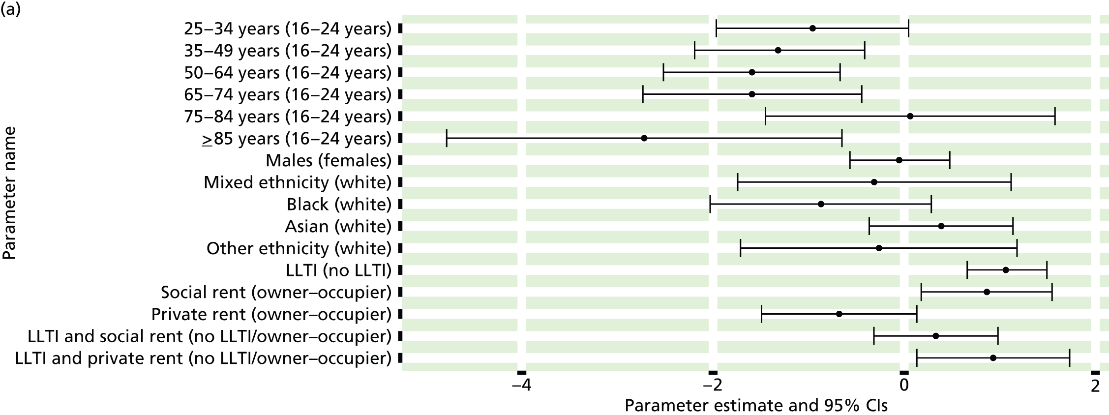

FIGURE 180.
Incidence of diagnosis of clinical depression: individual estimates and their 95% CIs. (a) MSOAs; (b) LAs; (c) CCGs; and (d) regions (GORs).


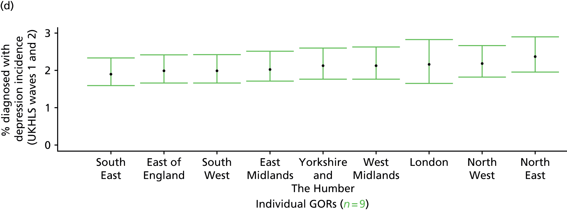
Incidence of diagnosis of current clinical depression (UK Household Longitudinal Survey, waves 1 and 2)
FIGURE 181.
Incidence of diagnosis of current clinical depression: LSOA-level map. Contains Ordnance Survey data © Crown copyright and database right 2012.
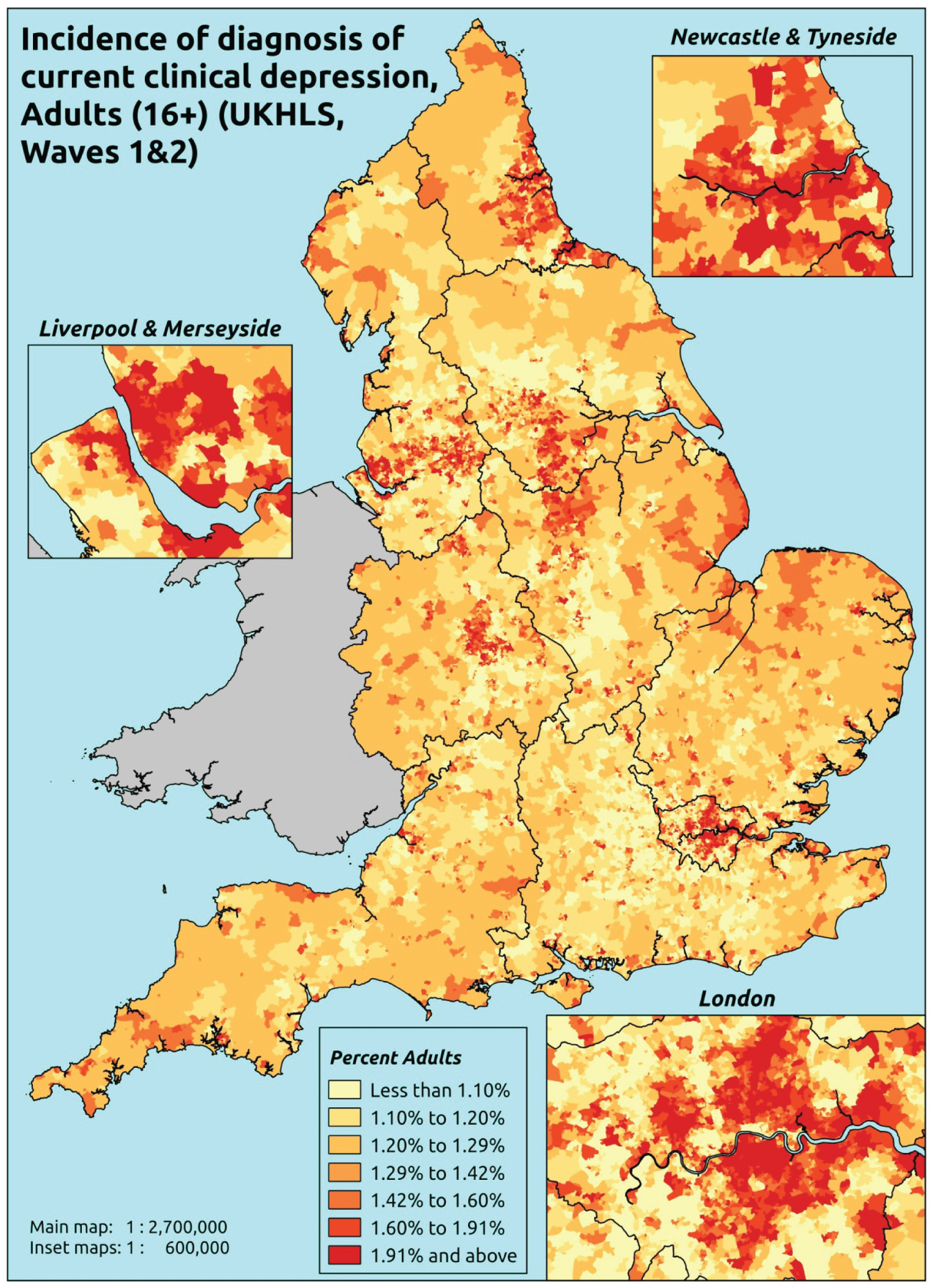
Response variable definition, provenance and prediction
Based on the question asked of respondents to the second wave of the UKHLS, ‘Have you been diagnosed since your last interview and still have clinical depression’, this provides an approximate estimate of the incidence of the diagnosis of clinical depression of people who, at the time of their interview, still have clinical depression. As noted above, people diagnosed with clinical depression prior to their first wave interview will answer ‘no’ to this question so this measure cannot be used as a marker of the prevalence of clinical depression. Moreover, as also noted above, the time interval between individuals’ interviews varies, albeit around a mean of 12.2 months. This can perhaps be seen as providing the basis for estimating the incidence of ‘unresolved’ doctor-diagnosed clinical depression – which is probably too specific to be of particular use, as a proxy for health-care needs. As this explicitly refers to a doctor diagnosis, this measure of incidence will reflect any sociodemographic or geographic variations in access to, or uptake of, care.
The first wave of the UKHLS data set (n = 50,994) runs from January 2009 to January 2011 and includes multiple household respondents aged ≥ 16 years from across the UK. The second wave (n = 31,242) runs from January 2010 to January 2012 and similarly comprises multiple household respondents aged ≥ 16 years from across the UK. Here the analytical data set is drawn from the subset of second wave respondents living in England who were also interviewed during the first wave and for whom data are available across all model response and predictor variables, namely that they reported (in the second wave questionnaire) whether or not they still had clinical depression which had been diagnosed since their last interview, along with information on age band, sex, ethnicity, LLTI, tenure and the IMD score of the LSOA of residence (n = 17,614). A single randomly selected adult is then drawn from each household, resulting in an analytical data set of 11,448 adults aged ≥ 16. (Note that in this instance we do not require a valid response to the first wave question about ever having been diagnosed with clinical depression.)
| Age band (years) | Females | Age band (years) | Males | ||||
|---|---|---|---|---|---|---|---|
| Does not have condition | Has condition | % | Does not have condition | Has condition | % | ||
| 16–24 | 456 | 10 | 2.1 | 16–24 | 338 | 5 | 1.5 |
| 25–34 | 1044 | 16 | 1.5 | 25–34 | 694 | 7 | 1.0 |
| 35–49 | 1903 | 43 | 2.2 | 35–49 | 1274 | 16 | 1.2 |
| 50–64 | 1668 | 32 | 1.9 | 50–64 | 1164 | 14 | 1.2 |
| 65–74 | 845 | 10 | 1.2 | 65–74 | 651 | 6 | 0.9 |
| 75–84 | 574 | 4 | 0.7 | 75–84 | 368 | 2 | 0.5 |
| ≥ 85 | 189 | 1 | 0.5 | ≥ 85 | 114 | 0 | 0.0 |
| Females | 6679 | 116 | 1.7 | Males | 4603 | 50 | 1.1 |
| Total (males and females) | 11,282 | 166 | 1.5 | ||||
Model parameters are applied to microsimulated LSOA-level census data to produce estimates of the number (and proportion) of people expected to be diagnosed with clinical depression during a 12-month period in each age–sex cohort (and overall) in each of the 32,844 English LSOAs. As discussed in the report, bootstrapping is used to derive 95% CIs for the estimates. These LSOA-level prevalence rate estimates (and 95% CIs) are aggregated into a number of higher geographies, namely MSOAs, LAs, CCGs and regions (GORs). Proportionate attribution is used to restructure the prevalence rate estimates to align with 2001 MSOAs, as well as GP practice populations as defined by the 2011 NHS ADS.
Table 203 summarises how expected prevalence rates vary by age, sex and local deprivation (as measured by the 2010 IMD). There are 6569 LSOAs (with 9,226,227 adults) classified as being in the least deprived quintile; 6568 LSOAs (9,525,344 adults) in the second least deprived quintile; 6568 LSOAs (9,658,444 adults) in the third least deprived quintile; 6568 LSOAs (9,650,576 adults) in the fourth least deprived quintile; and 6568 LSOAs (9,535,167 adults) in the most deprived quintile. Note that, as a general rule, variations in prevalence rates reflect variations in the socioeconomic composition of populations in the different types of LSOA rather than variations in deprivation per se.
| Cohort | Least deprived quintile LSOAs | Second least deprived quintile LSOAs | Third least deprived quintile LSOAs | Fourth least deprived quintile LSOAs | Most deprived quintile LSOAs | All England |
|---|---|---|---|---|---|---|
| Female 16–24 | 1.9 (0.8 to 2.8) | 2.0 (0.9 to 2.8) | 2.1 (0.9 to 3.0) | 2.3 (1.0 to 3.5) | 2.7 (1.2 to 4.1) | 2.3 (1.0 to 3.3) |
| Female 25–34 | 0.9 (0.5 to 1.5) | 1.0 (0.5 to 1.5) | 1.0 (0.5 to 1.6) | 1.2 (0.6 to 1.8) | 1.4 (0.8 to 2.3) | 1.1 (0.6 to 1.8) |
| Female 35–49 | 1.0 (0.7 to 1.4) | 1.1 (0.8 to 1.5) | 1.3 (0.9 to 1.7) | 1.5 (1.1 to 2.1) | 2.0 (1.4 to 2.8) | 1.4 (1.0 to 1.9) |
| Female 50–64 | 1.0 (0.6 to 1.4) | 1.1 (0.7 to 1.6) | 1.3 (0.8 to 1.8) | 1.6 (1.0 to 2.2) | 2.1 (1.3 to 3.0) | 1.4 (0.9 to 1.9) |
| Female 65–74 | 1.5 (0.7 to 2.3) | 1.6 (0.7 to 2.6) | 1.8 (0.8 to 2.9) | 2.1 (1.0 to 3.5) | 2.8 (1.3 to 4.7) | 1.9 (0.9 to 3.1) |
| Female ≥ 75 | 1.4 (0.5 to 2.8) | 1.5 (0.6 to 3.0) | 1.7 (0.6 to 3.3) | 1.9 (0.7 to 3.8) | 2.4 (0.9 to 4.8) | 1.7 (0.7 to 3.5) |
| Females | 1.2 (0.6 to 1.9) | 1.3 (0.7 to 2.0) | 1.4 (0.8 to 2.2) | 1.7 (0.9 to 2.6) | 2.1 (1.2 to 3.4) | 1.6 (0.9 to 2.4) |
| Male 16–24 | 1.7 (0.7 to 2.7) | 1.7 (0.7 to 2.8) | 1.8 (0.8 to 2.9) | 2.0 (0.9 to 3.2) | 2.4 (1.1 to 3.8) | 2.0 (0.9 to 3.1) |
| Male 25–34 | 0.8 (0.4 to 1.3) | 0.8 (0.4 to 1.4) | 0.9 (0.4 to 1.5) | 1.0 (0.5 to 1.7) | 1.2 (0.6 to 2.2) | 1.0 (0.5 to 1.7) |
| Male 35–49 | 0.9 (0.5 to 1.4) | 0.9 (0.6 to 1.6) | 1.1 (0.7 to 1.8) | 1.3 (0.8 to 2.2) | 1.7 (1.1 to 2.9) | 1.2 (0.8 to 2.0) |
| Male 50–64 | 0.8 (0.6 to 1.3) | 0.9 (0.6 to 1.5) | 1.1 (0.7 to 1.7) | 1.3 (0.9 to 2.1) | 1.8 (1.1 to 2.8) | 1.2 (0.8 to 1.8) |
| Male 65–74 | 1.2 (0.6 to 2.1) | 1.3 (0.7 to 2.4) | 1.5 (0.8 to 2.7) | 1.8 (1.0 to 3.3) | 2.3 (1.2 to 4.4) | 1.6 (0.8 to 2.9) |
| Male ≥ 75 | 1.3 (0.5 to 2.7) | 1.4 (0.5 to 2.9) | 1.5 (0.6 to 3.1) | 1.8 (0.7 to 3.7) | 2.2 (0.9 to 4.5) | 1.6 (0.6 to 3.3) |
| Males | 1.0 (0.6 to 1.8) | 1.1 (0.6 to 1.9) | 1.2 (0.7 to 2.1) | 1.4 (0.8 to 2.5) | 1.8 (1.0 to 3.1) | 1.3 (0.7 to 2.3) |
| All | 1.1 (0.9 to 1.4) | 1.2 (1.0 to 1.5) | 1.3 (1.1 to 1.7) | 1.6 (1.3 to 2.0) | 2.0 (1.6 to 2.6) | 1.4 (1.2 to 1.8) |
| Factor (reference group) | Model coefficients | 95% CI | ||
|---|---|---|---|---|
| Estimate | SE | 2.5% CI | 97.50% | |
| (Intercept) | –4.11967 | 0.52972 | –5.15792 | –3.08142 |
| Age (16–24 years) | ||||
| 25–34 years | –0.88175 | 0.63640 | –2.12910 | 0.36560 |
| 35–49 years | –0.91742 | 0.54616 | –1.98788 | 0.15305 |
| 50–64 years | –1.13284 | 0.56338 | –2.23706 | –0.02862 |
| 65–74 years | –0.83686 | 0.65812 | –2.12678 | 0.45306 |
| 75–84 years | 0.08223 | 0.92754 | –1.73575 | 1.90021 |
| ≥ 85 years | –3.61552 | 2.03743 | –7.60888 | 0.37784 |
| Sex (females) | ||||
| Males | –0.05319 | 0.30397 | –0.64897 | 0.54260 |
| Ethnicity (white) | ||||
| Mixed | –0.00459 | 0.73326 | –1.44178 | 1.43261 |
| Black | –0.96635 | 0.72068 | –2.37889 | 0.44618 |
| Asian | 0.63062 | 0.39018 | –0.13414 | 1.39537 |
| Other | –0.01624 | 0.74296 | –1.47245 | 1.43996 |
| LLTI (no LTTI) | ||||
| LLTI | 1.13743 | 0.24735 | 0.65263 | 1.62222 |
| Tenure (owner–occupier) | ||||
| Social rent | 0.87918 | 0.40847 | 0.07858 | 1.67977 |
| Private rent or other tenure | –0.48197 | 0.48164 | –1.42598 | 0.46203 |
| LSOA deprivation score | ||||
| IMD score | –0.00650 | 0.01904 | –0.04382 | 0.03082 |
| Interaction effects | ||||
| 25–34 years by LSOA IMD | 0.01777 | 0.02139 | –0.02415 | 0.05969 |
| 35–49 years by LSOA IMD | 0.02792 | 0.01853 | –0.00840 | 0.06425 |
| 50–64 years by LSOA IMD | 0.02564 | 0.01909 | –0.01178 | 0.06306 |
| 65–74 years by LSOA IMD | –0.00856 | 0.02526 | –0.05807 | 0.04094 |
| 75–84 years by LSOA IMD | –0.15062 | 0.07907 | –0.30560 | 0.00436 |
| ≥ 85 years by LSOA IMD | 0.04136 | 0.06135 | –0.07889 | 0.16161 |
| LLTI and social rent | 0.32212 | 0.37705 | –0.41691 | 1.06114 |
| LLTI and private rent or other tenure | 1.16359 | 0.45993 | 0.26212 | 2.06506 |
| Social rent by LSOA IMD score | –0.00761 | 0.01119 | –0.02954 | 0.01433 |
| Private rent or other tenure by LSOA IMD score | 0.02005 | 0.01322 | –0.00585 | 0.04596 |
| Male by LSOA IMD | –0.01512 | 0.00990 | –0.03452 | 0.00427 |
FIGURE 182.
Parameter plots: incidence of diagnosis of current clinical depression.
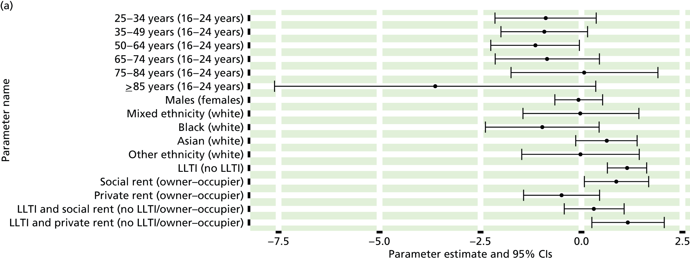

FIGURE 183.
Incidence of diagnosis of current clinical depression: individual estimates and their 95% CIs. (a) MSOAs; (b) LAs; (c) CCGs; and (d) regions (GORs).

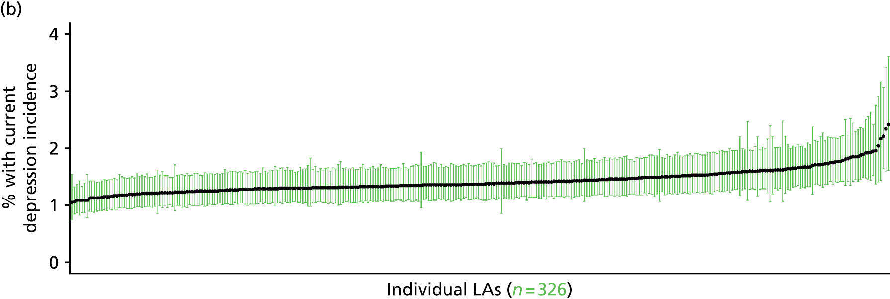
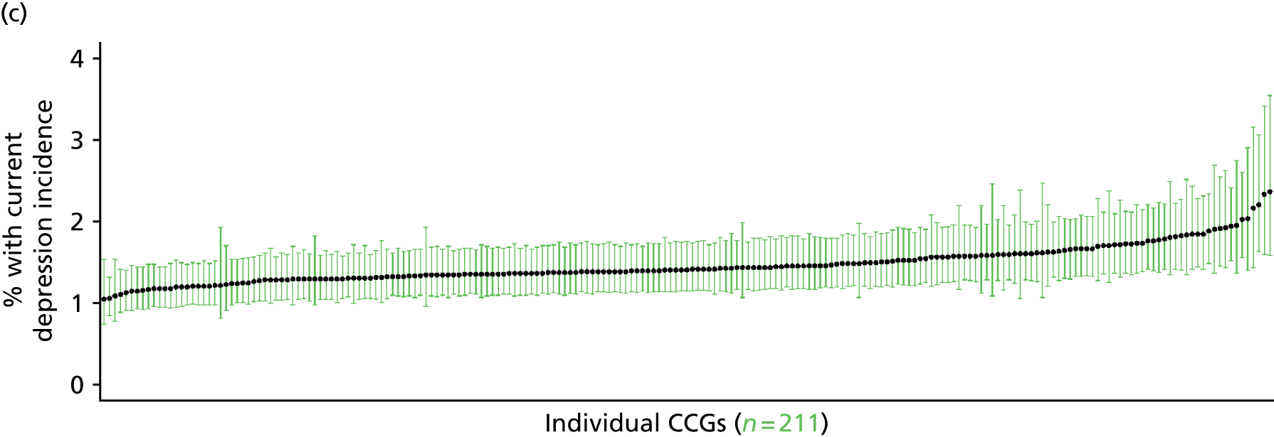
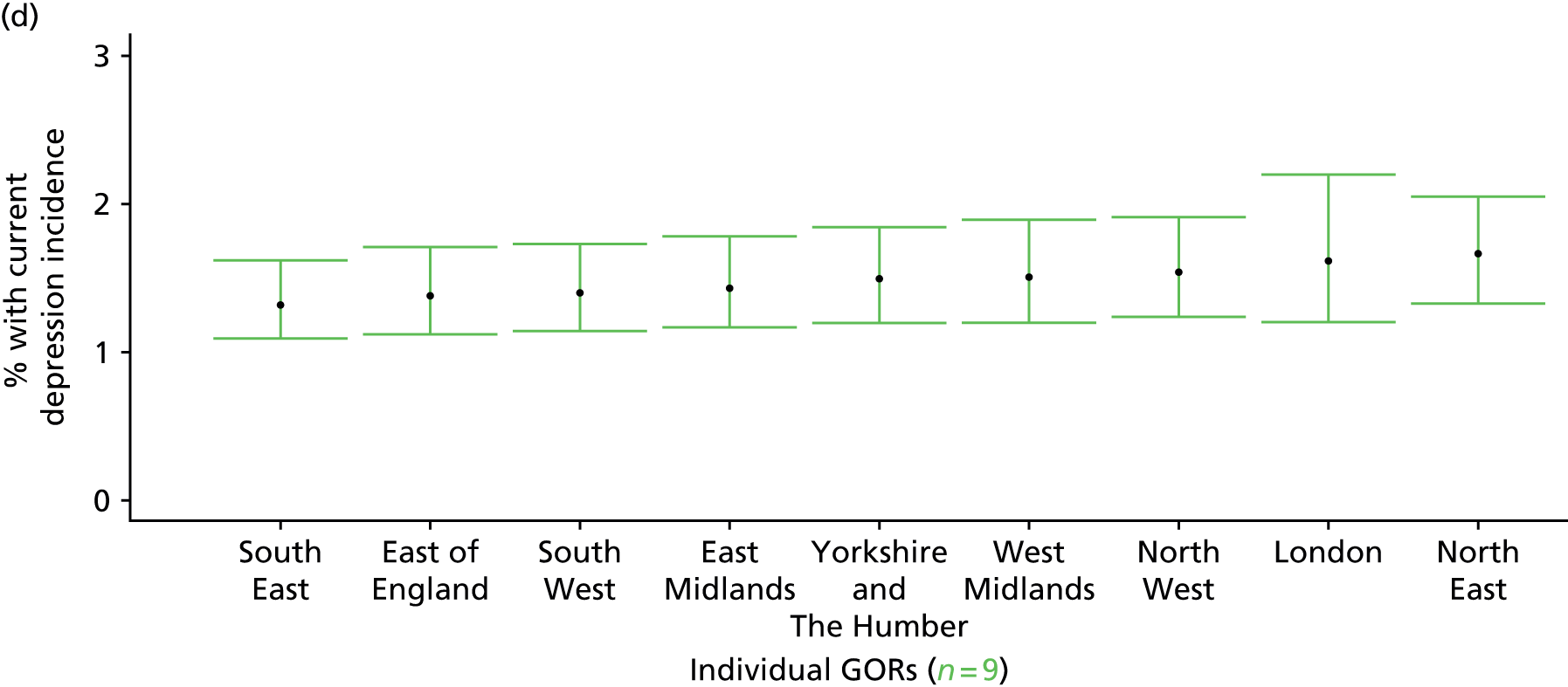
Self-reported moderate/extreme anxiety/depression (Health Survey for England, 2006, 2008 and 2010–11)
FIGURE 184.
Self-reported moderate/extreme anxiety/depression: LSOA-level map. Contains Ordnance Survey data © Crown copyright and database right 2012.

Response variable definition, provenance and prediction
Based on one of the questions in the EuroQol EQ-5D general health instrument, which was included in the HSfE in 2006, 2008 and 2010–11, respondents were asked to select one of the following options: (a) I am not anxious or depressed; (b) I am moderately anxious or depressed; or (c) I am extremely anxious or depressed. Here we capture those who have responded ‘yes’ to either (b) or (c). This is not entirely independent of sociodemographic or geographic variations in access to, or uptake of, care, as individuals may be able to state that they are not anxious or depressed because they are currently being treated (see the alternative marker below which describes the prevalence of moderate or extreme anxiety/depression which includes people currently being treated).
The HSfE at this time includes multiple household respondents of all ages. The analytical data set is drawn from a subset of respondents aged ≥ 16 years for whom data are available across all model response and predictor variables, namely whether or not they responded to this EuroQol EQ-5D question, along with information on age band, sex, ethnicity, general health status, LLTI, tenure and the IMD quintile of the LSOA of residence (n = 42,287). A single randomly selected adult is then drawn from each household, resulting in an analytical data set of 23,822 adults aged ≥ 16 years.
| Age band (years) | Females | Age band (years) | Males | ||||
|---|---|---|---|---|---|---|---|
| Does not have condition | Has condition | % | Does not have condition | Has condition | % | ||
| 16–24 | 899 | 216 | 19.4 | 16–24 | 644 | 108 | 14.4 |
| 25–34 | 1670 | 454 | 21.4 | 25–34 | 1130 | 245 | 17.8 |
| 35–49 | 2873 | 842 | 22.7 | 35–49 | 2126 | 516 | 19.5 |
| 50–64 | 2471 | 907 | 26.9 | 50–64 | 2006 | 577 | 22.3 |
| 65–74 | 1370 | 449 | 24.7 | 65–74 | 1181 | 221 | 15.8 |
| 75–84 | 1009 | 348 | 25.6 | 75–84 | 698 | 157 | 18.4 |
| ≥ 85 | 336 | 145 | 30.1 | ≥ 85 | 160 | 64 | 28.6 |
| Females | 10,628 | 3361 | 24.0 | Males | 7945 | 1888 | 19.2 |
| Total (males and females) | 18,573 | 5249 | 22.0 | ||||
Model parameters are applied to microsimulated LSOA-level census data to produce estimates of the number (and proportion) of people expected to report moderate or extreme anxiety and/or depression in each age–sex cohort (and overall) in each of the 32,844 English LSOAs. As discussed in the report, bootstrapping is used to derive 95% CIs for the estimates. These LSOA-level prevalence rate estimates (and 95% CIs) are aggregated into a number of higher geographies, namely MSOAs, LAs, CCGs and regions (GORs). Proportionate attribution is used to restructure the prevalence rate estimates to align with 2001 MSOAs, as well as GP practice populations as defined by the 2011 NHS ADS.
Table 206 summarises how expected prevalence rates vary by age, sex and local deprivation (as measured by the 2010 IMD). There are 6569 LSOAs (with 9,226,227 adults) classified as being in the least deprived quintile; 6568 LSOAs (9,525,344 adults) in the second least deprived quintile; 6568 LSOAs (9,658,444 adults) in the third least deprived quintile; 6568 LSOAs (9,650,576 adults) in the fourth least deprived quintile; and 6568 LSOAs (9,535,167 adults) in the most deprived quintile. Note that, as a general rule, variations in prevalence rates reflect variations in the socioeconomic composition of populations in the different types of LSOA rather than variations in deprivation per se.
| Cohort | Least deprived quintile LSOAs | Second least deprived quintile LSOAs | Third least deprived quintile LSOAs | Fourth least deprived quintile LSOAs | Most deprived quintile LSOAs | All England |
|---|---|---|---|---|---|---|
| Female 16–24 | 13.6 (11.2 to 15.4) | 13.6 (11.7 to 15.5) | 15.3 (13.1 to 17.1) | 15.3 (13.3 to 17.3) | 16.9 (14.8 to 18.5) | 15.2 (13.2 to 16.8) |
| Female 25–34 | 14.4 (12.9 to 15.6) | 14.8 (13.5 to 16.3) | 17.0 (15.5 to 18.4) | 18.1 (16.4 to 19.6) | 21.2 (19.5 to 22.8) | 17.6 (16.2 to 18.9) |
| Female 35–49 | 18.3 (17.0 to 19.6) | 19.5 (18.4 to 20.8) | 23.1 (21.8 to 24.4) | 25.4 (23.9 to 26.8) | 30.8 (28.9 to 32.5) | 23.4 (22.3 to 24.5) |
| Female 50–64 | 23.3 (21.9 to 24.7) | 24.9 (23.4 to 26.4) | 29.3 (27.6 to 30.6) | 32.5 (30.7 to 34.1) | 39.8 (37.7 to 41.5) | 29.5 (28.1 to 30.6) |
| Female 65–74 | 23.6 (21.5 to 25.8) | 25.1 (23.1 to 26.9) | 28.8 (26.8 to 30.9) | 31.3 (28.8 to 33.5) | 36.7 (33.7 to 39.2) | 28.5 (26.5 to 30.3) |
| Female ≥ 75 | 30.8 (28.7 to 33.3) | 31.6 (29.3 to 34.1) | 34.5 (32.0 to 36.8) | 35.3 (33.2 to 37.8) | 38.2 (35.6 to 41.0) | 33.9 (32.0 to 36.1) |
| Females | 21.1 (19.4 to 22.7) | 22.0 (20.4 to 23.7) | 24.9 (23.1 to 26.5) | 25.9 (24.1 to 27.7) | 29.8 (27.7 to 31.7) | 24.8 (23.3 to 26.2) |
| Male 16–24 | 10.8 (8.6 to 12.6) | 10.8 (8.8 to 12.7) | 12.4 (10.0 to 14.1) | 12.3 (10.2 to 14.2) | 13.9 (11.7 to 16.0) | 12.2 (10.2 to 14.0) |
| Male 25–34 | 13.2 (11.8 to 14.5) | 13.5 (12.1 to 15.3) | 15.5 (13.9 to 17.2) | 16.2 (14.8 to 17.9) | 19.4 (17.4 to 21.5) | 16.0 (14.6 to 17.6) |
| Male 35–49 | 14.9 (13.8 to 16.0) | 16.0 (14.9 to 17.3) | 19.1 (17.8 to 20.4) | 21.3 (19.8 to 23.0) | 26.6 (25.2 to 28.4) | 19.6 (18.5 to 20.8) |
| Male 50–64 | 18.1 (16.6 to 19.4) | 19.9 (18.4 to 21.2) | 23.9 (22.0 to 25.3) | 27.3 (25.3 to 28.8) | 34.4 (31.9 to 36.4) | 24.3 (22.6 to 25.6) |
| Male 65–74 | 14.9 (13.3 to 16.9) | 16.1 (14.6 to 18.1) | 19.2 (17.4 to 21.6) | 21.4 (19.5 to 23.8) | 25.9 (23.7 to 28.8) | 19.0 (17.4 to 21.1) |
| Male ≥ 75 | 23.1 (20.4 to 25.0) | 23.9 (21.5 to 26.1) | 26.6 (24.0 to 28.7) | 27.3 (24.6 to 30.1) | 30.3 (27.5 to 33.0) | 25.9 (23.4 to 28.0) |
| Males | 16.0 (14.4 to 17.4) | 16.9 (15.4 to 18.5) | 19.5 (17.7 to 21.2) | 20.8 (18.9 to 22.6) | 24.9 (22.8 to 27.0) | 19.6 (18.1 to 21.2) |
| All | 18.6 (17.6 to 19.5) | 19.6 (18.8 to 20.5) | 22.3 (21.3 to 23.1) | 23.4 (22.5 to 24.4) | 27.4 (26.2 to 28.5) | 22.3 (21.8 to 22.8) |
| Factor (reference group) | Model coefficients | 95% CI | ||
|---|---|---|---|---|
| Estimate | SE | 2.5% CI | 97.50% | |
| (Intercept) | –2.35267 | 0.12570 | –2.59903 | –2.10630 |
| Age (16–24 years) | ||||
| 25–34 years | –0.07016 | 0.13640 | –0.33750 | 0.19719 |
| 35–49 years | 0.04530 | 0.12323 | –0.19624 | 0.28683 |
| 50–64 years | 0.05842 | 0.12301 | –0.18268 | 0.29952 |
| 65–74 years | –0.10321 | 0.13134 | –0.36064 | 0.15422 |
| 75–84 years | –0.18033 | 0.13866 | –0.45211 | 0.09145 |
| ≥ 85 years | 0.10935 | 0.17036 | –0.22455 | 0.44324 |
| Sex (females) | ||||
| Males | –0.16364 | 0.15150 | –0.46059 | 0.13330 |
| Ethnicity (white) | ||||
| Mixed | 0.14685 | 0.19518 | –0.23570 | 0.52941 |
| Black | –0.11681 | 0.09934 | –0.31153 | 0.07790 |
| Asian | –0.32077 | 0.13632 | –0.58796 | –0.05357 |
| Other | 0.19295 | 0.27256 | –0.34126 | 0.72717 |
| General health status (very good health) | ||||
| Good health | 0.80504 | 0.06095 | 0.68558 | 0.92449 |
| Fair health | 1.48262 | 0.07000 | 1.34542 | 1.61983 |
| Bad health | 2.11738 | 0.09684 | 1.92757 | 2.30719 |
| Very bad health | 2.61408 | 0.15356 | 2.31309 | 2.91506 |
| LLTI (no LTTI) | ||||
| LLTI | 0.50794 | 0.04362 | 0.42245 | 0.59343 |
| Tenure (owner–occupier) | ||||
| Social rent | 0.12904 | 0.15792 | –0.18048 | 0.43855 |
| Private rent or other tenure | 0.14439 | 0.15223 | –0.15397 | 0.44276 |
| LSOA deprivation quintile (least deprived quintile) | ||||
| Second LSOA deprivation quintile | –0.03083 | 0.05527 | –0.13915 | 0.07749 |
| Third LSOA deprivation quintile | 0.07159 | 0.05445 | –0.03513 | 0.17831 |
| Fourth LSOA deprivation quintile | 0.02644 | 0.05587 | –0.08307 | 0.13595 |
| Fifth LSOA deprivation quintile ( = most deprived) | 0.07720 | 0.05854 | –0.03753 | 0.19194 |
| Interaction effects | ||||
| 25–34 years and social rent | 0.44347 | 0.19416 | 0.06292 | 0.82403 |
| 35–49 years and social rent | 0.41431 | 0.17771 | 0.06599 | 0.76262 |
| 50–64 years and social rent | 0.28633 | 0.17830 | –0.06315 | 0.63580 |
| 65–74 years and social rent | –0.22477 | 0.19558 | –0.60810 | 0.15856 |
| 75–84 years and social rent | –0.27405 | 0.20052 | –0.66707 | 0.11897 |
| ≥ 85 years and social rent | –0.47514 | 0.25036 | –0.96585 | 0.01557 |
| 25–34 years and private rent or other tenure | 0.33057 | 0.18466 | –0.03135 | 0.69250 |
| 35–49 years and private rent or other tenure | 0.31291 | 0.17955 | –0.03902 | 0.66484 |
| 50–64 years and private rent or other tenure | 0.24802 | 0.19877 | –0.14157 | 0.63762 |
| 65–74 years and private rent or other tenure | 0.05444 | 0.26081 | –0.45674 | 0.56562 |
| 75–84 years and private rent or other tenure | –0.62048 | 0.32221 | –1.25201 | 0.01105 |
| ≥ 85 years and private rent or other tenure | –0.94228 | 0.52153 | –1.96448 | 0.07993 |
| 25–34 years and male | 0.12056 | 0.16428 | –0.20142 | 0.44254 |
| 35–49 years and male | 0.00340 | 0.15086 | –0.29228 | 0.29908 |
| 50–64 years and male | –0.10746 | 0.15172 | –0.40483 | 0.18991 |
| 65–74 years and male | –0.47117 | 0.16866 | –0.80175 | –0.14059 |
| 75–84 years and male | –0.33054 | 0.18082 | –0.68495 | 0.02387 |
| ≥ 85 and male | 0.05275 | 0.23644 | –0.41067 | 0.51616 |
| Mixed and LLTI | –0.59751 | 0.37502 | –1.33255 | 0.13754 |
| Black and LLTI | 0.54932 | 0.18473 | 0.18725 | 0.91139 |
| Asian and LLTI | 0.15753 | 0.25551 | –0.34327 | 0.65834 |
| Other and LLTI | –0.08964 | 0.57721 | –1.22097 | 1.04169 |
| Male and good health | –0.18440 | 0.10060 | –0.38158 | 0.01278 |
| Male and fair health | 0.04090 | 0.10869 | –0.17213 | 0.25394 |
| Male and bad health | 0.19159 | 0.14549 | –0.09357 | 0.47675 |
| Male and very bad health | 0.01818 | 0.23288 | –0.43826 | 0.47463 |
FIGURE 185.
Parameter plots: self-reported moderate/extreme anxiety/depression.

FIGURE 186.
Self-reported moderate/extreme anxiety/depression: individual estimates and their 95% CIs. (a) MSOAs; (b) LAs; (c) CCGs; and (d) regions (GORs).
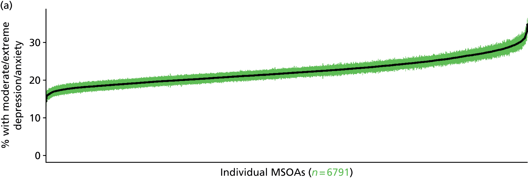

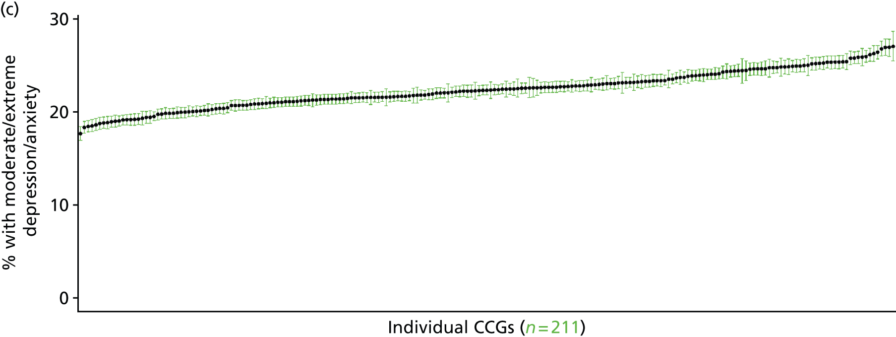
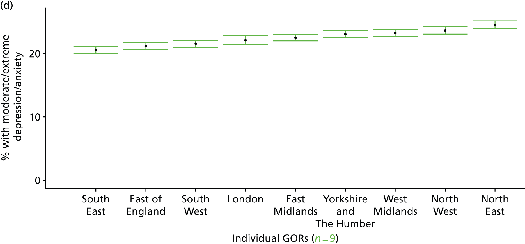
Self-reported extreme anxiety/depression (Health Survey for England, 2006, 2008 and 2010–11)
FIGURE 187.
Self-reported extreme anxiety/depression: LSOA-level map. Contains Ordnance Survey data © Crown copyright and database right 2012.
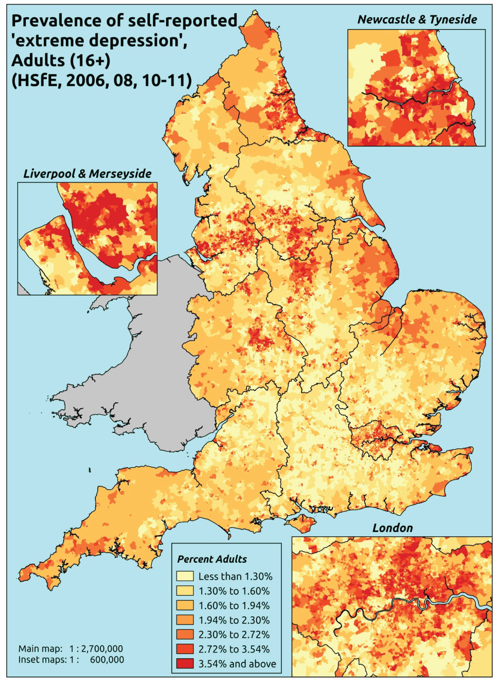
Response variable definition, provenance and prediction
Based on one of the questions in the EuroQol EQ-5D General Health instrument, which was included in the HSfE in 2006, 2008 and 2010–11, respondents were asked to select one of the following options: (a) I am not anxious or depressed; (b) I am moderately anxious or depressed; or (c) I am extremely anxious or depressed. Here we capture those who have responded ‘yes’ to (c). This is not entirely independent of sociodemographic or geographic variations in access to, or uptake of, care, as individuals may be able to state that they are not anxious or depressed because they are currently being treated (see the alternative marker below which describes the prevalence of extreme anxiety/depression which includes people currently being treated).
The HSfE at this time includes multiple household respondents of all ages. The analytical data set is drawn from a subset of respondents aged ≥ 16 years for whom data are available across all model response and predictor variables, namely whether or not they responded to this EuroQol EQ-5D question, along with information on age band, sex, ethnicity, general health status, LLTI, tenure and the IMD quintile of the LSOA of residence (n = 42,287). A single randomly selected adult is then drawn from each household, resulting in an analytical data set of 23,822 adults aged ≥ 16 years.
| Age band (years) | Females | Age band (years) | Males | ||||
|---|---|---|---|---|---|---|---|
| Does not have condition | Has condition | % | Does not have condition | Has condition | % | ||
| 16–24 | 1095 | 20 | 1.8 | 16–24 | 741 | 11 | 1.5 |
| 25–34 | 2073 | 51 | 2.4 | 25–34 | 1348 | 27 | 2.0 |
| 35–49 | 3623 | 92 | 2.5 | 35–49 | 2578 | 64 | 2.4 |
| 50–64 | 3259 | 119 | 3.5 | 50–64 | 2514 | 69 | 2.7 |
| 65–74 | 1786 | 33 | 1.8 | 65–74 | 1386 | 16 | 1.1 |
| 75–84 | 1336 | 21 | 1.5 | 75–84 | 840 | 15 | 1.8 |
| ≥ 85 | 473 | 8 | 1.7 | ≥ 85 | 220 | 4 | 1.8 |
| Females | 13,645 | 344 | 2.5 | Males | 9627 | 206 | 2.1 |
| Total (males and females) | 23,272 | 550 | 2.3 | ||||
Model parameters are applied to microsimulated LSOA-level census data to produce estimates of the number (and proportion) of people expected to report extreme anxiety and/or depression in each age–sex cohort (and overall) in each of the 32,844 English LSOAs. As discussed in the report, bootstrapping is used to derive 95% CIs for the estimates. These LSOA-level prevalence rate estimates (and 95% CIs) are aggregated into a number of higher geographies, namely MSOAs, LAs, CCGs and regions (GORs). Proportionate attribution is used to restructure the prevalence rate estimates to align with 2001 MSOAs, as well as GP practice populations as defined by the 2011 NHS ADS.
Table 209 summarises how expected prevalence rates vary by age, sex and local deprivation (as measured by the 2010 IMD). There are 6569 LSOAs (with 9,226,227 adults) classified as being in the least deprived quintile; 6568 LSOAs (9,525,344 adults) in the second least deprived quintile; 6568 LSOAs (9,658,444 adults) in the third least deprived quintile; 6568 LSOAs (9,650,576 adults) in the fourth least deprived quintile; and 6568 LSOAs (9,535,167 adults) in the most deprived quintile. Note that, as a general rule, variations in prevalence rates reflect variations in the socioeconomic composition of populations in the different types of LSOA rather than variations in deprivation per se.
| Cohort | Least deprived quintile LSOAs | Second least deprived quintile LSOAs | Third least deprived quintile LSOAs | Fourth least deprived quintile LSOAs | Most deprived quintile LSOAs | All England |
|---|---|---|---|---|---|---|
| Female 16–24 | 1.0 (0.6 to 1.3) | 0.9 (0.6 to 1.2) | 1.5 (1.0 to 1.9) | 1.3 (0.9 to 1.7) | 1.8 (1.3 to 2.3) | 1.3 (1.0 to 1.7) |
| Female 25–34 | 1.2 (0.9 to 1.6) | 1.1 (0.9 to 1.5) | 1.9 (1.5 to 2.4) | 1.8 (1.4 to 2.2) | 2.6 (2.0 to 3.1) | 1.8 (1.5 to 2.2) |
| Female 35–49 | 1.5 (1.1 to 1.9) | 1.5 (1.2 to 2.0) | 3.0 (2.4 to 3.5) | 3.1 (2.3 to 3.8) | 4.8 (3.8 to 5.6) | 2.8 (2.4 to 3.2) |
| Female 50–64 | 2.0 (1.6 to 2.6) | 2.0 (1.5 to 2.7) | 4.0 (3.1 to 4.7) | 4.1 (3.3 to 5.2) | 6.6 (5.2 to 7.6) | 3.6 (3.1 to 4.1) |
| Female 65–74 | 1.3 (0.9 to 1.9) | 1.3 (0.9 to 1.9) | 2.4 (1.8 to 3.2) | 2.4 (1.7 to 3.3) | 3.7 (2.8 to 5.0) | 2.1 (1.7 to 2.8) |
| Female ≥ 75 | 1.8 (1.3 to 2.6) | 1.6 (1.1 to 2.4) | 2.9 (2.1 to 3.9) | 2.6 (1.9 to 3.4) | 3.4 (2.5 to 4.6) | 2.4 (1.9 to 3.1) |
| Females | 1.6 (1.2 to 2.1) | 1.5 (1.1 to 2.1) | 2.8 (2.2 to 3.5) | 2.7 (2.0 to 3.4) | 4.0 (3.1 to 4.8) | 2.5 (2.1 to 3.0) |
| Male 16–24 | 0.5 (0.3 to 0.9) | 1.0 (0.6 to 1.3) | 0.8 (0.5 to 1.3) | 1.2 (0.9 to 1.6) | 1.8 (1.3 to 2.4) | 1.1 (0.8 to 1.5) |
| Male 25–34 | 0.7 (0.5 to 1.1) | 1.3 (0.9 to 1.7) | 1.1 (0.7 to 1.6) | 1.6 (1.2 to 2.0) | 2.7 (2.1 to 3.2) | 1.6 (1.3 to 1.9) |
| Male 35–49 | 0.8 (0.5 to 1.2) | 1.7 (1.2 to 2.2) | 1.6 (1.2 to 2.2) | 2.7 (2.1 to 3.3) | 4.8 (3.7 to 5.7) | 2.3 (2.0 to 2.7) |
| Male 50–64 | 1.2 (0.7 to 1.7) | 2.5 (1.8 to 3.2) | 2.4 (1.6 to 3.2) | 4.0 (3.1 to 5.0) | 6.8 (5.2 to 8.0) | 3.2 (2.8 to 3.6) |
| Male 65–74 | 0.8 (0.5 to 1.2) | 1.6 (1.1 to 2.3) | 1.4 (1.0 to 2.2) | 2.3 (1.7 to 3.3) | 3.8 (2.8 to 5.3) | 1.9 (1.5 to 2.4) |
| Male ≥ 75 | 1.0 (0.6 to 1.6) | 1.9 (1.2 to 2.8) | 1.6 (1.0 to 2.3) | 2.3 (1.7 to 3.3) | 3.4 (2.4 to 4.8) | 1.9 (1.5 to 2.5) |
| Males | 0.9 (0.5 to 1.3) | 1.8 (1.2 to 2.4) | 1.6 (1.1 to 2.2) | 2.5 (1.9 to 3.2) | 4.1 (3.1 to 5.0) | 2.2 (1.8 to 2.6) |
| All | 1.2 (1.0 to 1.5) | 1.6 (1.3 to 2.0) | 2.2 (1.9 to 2.6) | 2.6 (2.2 to 3.0) | 4.0 (3.5 to 4.5) | 2.4 (2.2 to 2.5) |
| Factor (reference group) | Model coefficients | 95% CI | ||
|---|---|---|---|---|
| Estimate | SE | 2.5% CI | 97.50% | |
| (Intercept) | –7.07318 | 0.48360 | –8.02103 | –6.12533 |
| Age (16–24 years) | ||||
| 25–34 years | 0.49172 | 0.38612 | –0.26507 | 1.24852 |
| 35–49 years | 0.50278 | 0.36251 | –0.20774 | 1.21329 |
| 50–64 years | 0.41881 | 0.37274 | –0.31175 | 1.14937 |
| 65–74 years | –0.95315 | 0.55693 | –2.04474 | 0.13843 |
| 75–84 years | –0.62873 | 0.56042 | –1.72715 | 0.46968 |
| ≥ 85 years | 0.15193 | 0.61310 | –1.04975 | 1.35361 |
| Sex (females) | ||||
| Males | –0.56682 | 0.30913 | –1.17271 | 0.03907 |
| Ethnicity (white) | ||||
| Mixed | –0.40724 | 0.45431 | –1.2977 | 0.48321 |
| Black | –0.04028 | 0.22491 | –0.4811 | 0.40055 |
| Asian | –0.64900 | 0.37357 | –1.3812 | 0.08320 |
| Other | –0.04941 | 0.63893 | –1.30171 | 1.20289 |
| General health status (very good health) | ||||
| Good health | 1.26407 | 0.37143 | 0.53606 | 1.99208 |
| Fair health | 2.98812 | 0.36540 | 2.27194 | 3.70430 |
| Bad health | 4.54642 | 0.42986 | 3.70391 | 5.38894 |
| Very bad health | 4.61144 | 0.71974 | 3.20075 | 6.02214 |
| LLTI (no LTTI) | ||||
| LLTI | 3.26350 | 0.67990 | 1.93089 | 4.5961 |
| Tenure (owner–occupier) | ||||
| Social rent | 0.68126 | 0.11197 | 0.46180 | 0.90072 |
| Private rent or other tenure | 0.67180 | 0.14307 | 0.39138 | 0.95221 |
| LSOA deprivation quintile (least deprived quintile) | ||||
| Second LSOA deprivation quintile | –0.24950 | 0.23774 | –0.71548 | 0.21648 |
| Third LSOA deprivation quintile | 0.24804 | 0.21028 | –0.16412 | 0.66019 |
| Fourth LSOA deprivation quintile | –0.06075 | 0.21534 | –0.48282 | 0.36131 |
| Fifth LSOA deprivation quintile ( = most deprived) | 0.02917 | 0.20788 | –0.37828 | 0.43662 |
| Interaction effects | ||||
| Good health and LLTI | –0.66070 | 0.60767 | –1.85173 | 0.53033 |
| Fair health and LLTI | –1.45711 | 0.58771 | –2.60904 | –0.30519 |
| Bad health and LLTI | –2.00885 | 0.62929 | –3.24225 | –0.77545 |
| Very bad health and LLTI | –1.35961 | 0.85944 | –3.04411 | 0.32490 |
| 25–34 years and LLTI | –0.65846 | 0.48258 | –1.60432 | 0.28740 |
| 35–49 years and LLTI | –0.90168 | 0.44975 | –1.78320 | –0.02017 |
| 50–64 years and LLTI | –1.17807 | 0.45448 | –2.06884 | –0.28729 |
| 65–74 years and LLTI | –0.63567 | 0.62789 | –1.86633 | 0.59500 |
| 75–84 years and LLTI | –1.20204 | 0.63862 | –2.45374 | 0.04966 |
| ≥ 85 years and LLTI | –2.30358 | 0.75312 | –3.77970 | –0.82747 |
| Male and second LSOA deprivation quintile | 0.80773 | 0.39643 | 0.03074 | 1.58473 |
| Male and third LSOA deprivation quintile | –0.03841 | 0.38459 | –0.79222 | 0.71539 |
| Male and fourth LSOA deprivation quintile | 0.50386 | 0.36813 | –0.21767 | 1.22540 |
| Male and fifth LSOA deprivation quintile | 0.59010 | 0.34888 | –0.09370 | 1.27390 |
FIGURE 188.
Parameter plots: self-reported extreme anxiety/depression.
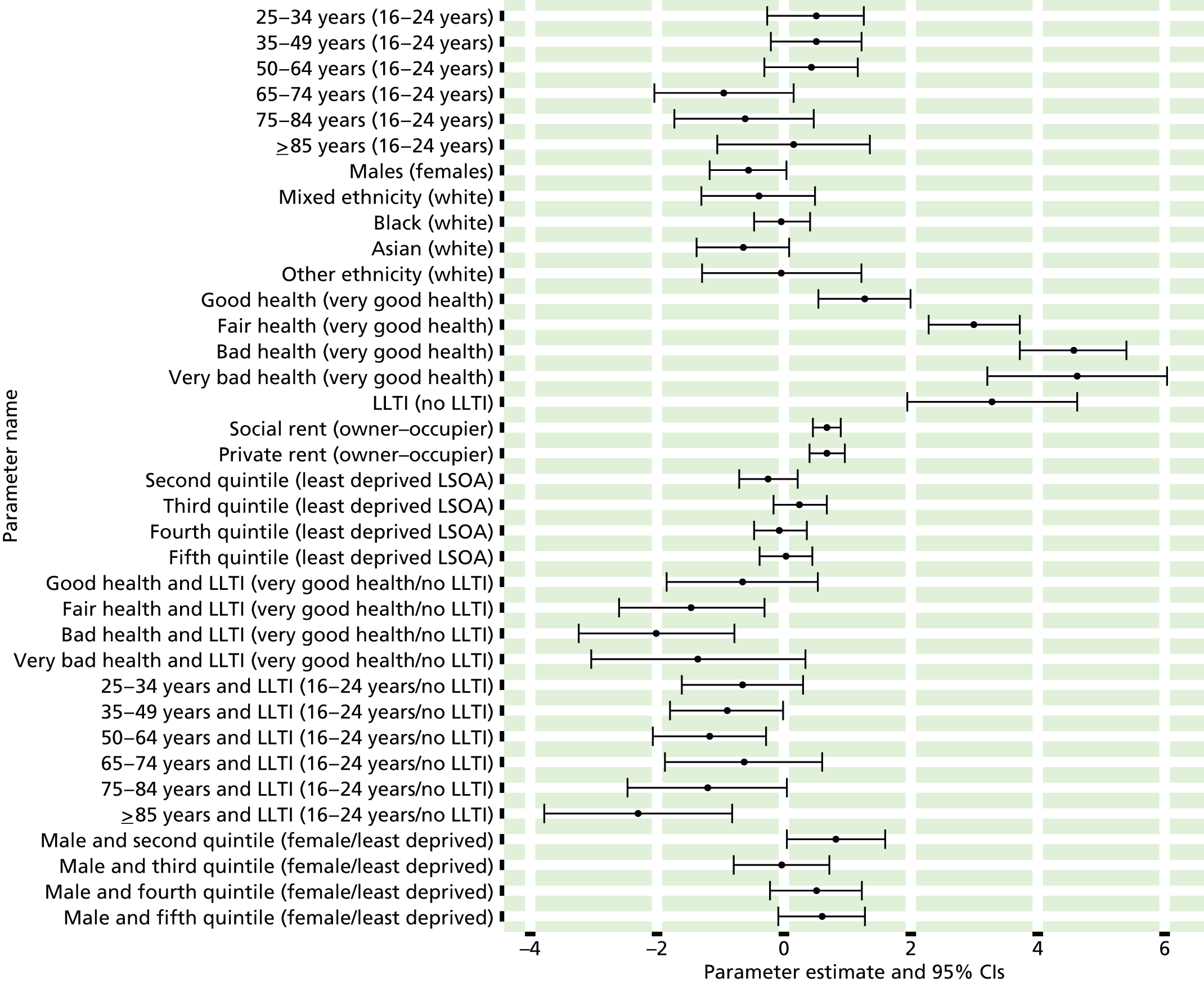
FIGURE 189.
Self-reported extreme anxiety/depression: individual estimates and their 95% CIs. (a) MSOAs; (b) LAs; (c) CCGs; and (d) regions (GORs).


Self-reported moderate/extreme anxiety/depression or currently prescribed anxiety/depression drugs (Health Survey for England, 2006, 2008, 2010–11)
FIGURE 190.
Self-reported moderate/extreme anxiety/depression or anxiety/depression drugs: LSOA-level map. Contains Ordnance Survey data © Crown copyright and database right 2012.
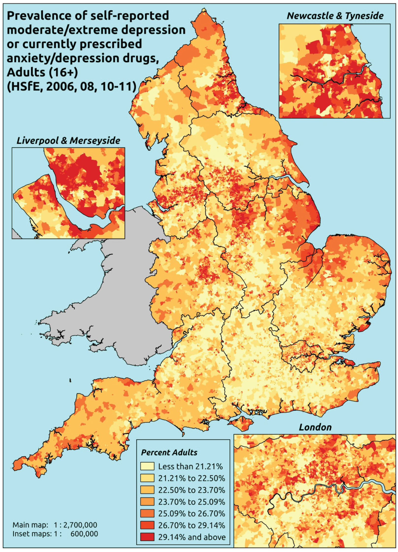
Response variable definition, provenance and prediction
Based on the recorded use of prescribed medication in addition to the EuroQol EQ-5D General Health instrument that was included in the HSfE in 2006, 2008 and 2010–11, respondents were asked to select one of the following options: (a) I am not anxious or depressed; (b) I am moderately anxious or depressed; or (c) I am extremely anxious or depressed. Here we capture those who have responded ‘yes’ to either (b) or (c) or who are currently prescribed drugs for depression and/or anxiety (BNF 4.1.1–4.1.3 or 4.3.1–4.3.4487). This aims to capture individuals would have answered that they were moderately or extremely anxious or depressed because they are receiving medication. There is no evidence available on whether they are receiving any other type of treatment. This marker of need is vulnerable to any sociodemographic or geographic variations in access to, or uptake of, care.
The HSfE at this time includes multiple household respondents of all ages. The analytical data set is drawn from a subset of respondents aged ≥ 16 years for whom data are available across all model response and predictor variables, namely: whether they responded to this EuroQol EQ-5D question, whether or not data are available on current prescriptions, along with information on age band, sex, ethnicity, general health status, LLTI, tenure and the IMD quintile of the LSOA of residence (n = 31,018). A single randomly selected adult is then drawn from each household, resulting in an analytical data set of 18,301 adults aged ≥ 16 years.
| Age band (years) | Females | Age band (years) | Males | ||||
|---|---|---|---|---|---|---|---|
| Does not have condition | Has condition | % | Does not have condition | Has condition | % | ||
| 16–24 | 607 | 140 | 18.7 | 16–24 | 437 | 67 | 13.3 |
| 25–34 | 1210 | 343 | 22.1 | 25–34 | 805 | 179 | 18.2 |
| 35–49 | 2084 | 805 | 27.9 | 35–49 | 1604 | 436 | 21.4 |
| 50–64 | 1901 | 811 | 29.9 | 50–64 | 1589 | 517 | 24.5 |
| 65–74 | 979 | 411 | 29.6 | 65–74 | 928 | 223 | 19.4 |
| 75–84 | 686 | 336 | 32.9 | 75–84 | 535 | 141 | 20.9 |
| ≥ 85 | 213 | 129 | 37.7 | ≥ 85 | 131 | 54 | 29.2 |
| Females | 7680 | 2975 | 27.9 | Males | 6029 | 1617 | 21.1 |
| Total (males and females) | 13,709 | 4592 | 25.1 | ||||
Model parameters are applied to microsimulated LSOA-level census data to produce estimates of the number (and proportion) of people expected to report moderate or extreme anxiety and/or depression or who are currently being prescribed drugs for depression and/or anxiety (BNF 4.1.1–4.1.3 or 4.3.1–4.3.4487) in each age–sex cohort (and overall) in each of the 32,844 English LSOAs. As discussed in the report, bootstrapping is used to derive 95% CIs for the estimates. These LSOA-level prevalence rate estimates (and 95% CIs) are aggregated into a number of higher geographies, namely MSOAs, LAs, CCGs and regions (GORs). Proportionate attribution is used to restructure the prevalence rate estimates to align with 2001 MSOAs, as well as GP practice populations as defined by the 2011 NHS ADS.
Table 212 summarises how expected prevalence rates vary by age, sex and local deprivation (as measured by the 2010 IMD). There are 6569 LSOAs (with 9,226,227 adults) classified as being in the least deprived quintile; 6568 LSOAs (9,525,344 adults) in the second least deprived quintile; 6568 LSOAs (9,658,444 adults) in the third least deprived quintile; 6568 LSOAs (9,650,576 adults) in the fourth least deprived quintile; and 6568 LSOAs (9,535,167 adults) in the most deprived quintile. Note that, as a general rule, variations in prevalence rates reflect variations in the socioeconomic composition of populations in the different types of LSOA rather than variations in deprivation per se.
| Cohort | Least deprived quintile LSOAs | Second least deprived quintile LSOAs | Third least deprived quintile LSOAs | Fourth least deprived quintile LSOAs | Most deprived quintile LSOAs | All England |
|---|---|---|---|---|---|---|
| Female 16–24 | 14.6 (12.6 to 17.1) | 14.1 (12.1 to 16.5) | 15.5 (13.5 to 17.7) | 15.0 (13.0 to 17.1) | 16.8 (14.6 to 18.6) | 15.3 (13.5 to 17.5) |
| Female 25–34 | 15.4 (14.1 to 16.9) | 15.3 (14.2 to 17.1) | 17.8 (16.4 to 19.3) | 18.5 (17.2 to 20.3) | 22.2 (20.5 to 24.1) | 18.4 (17.2 to 19.9) |
| Female 35–49 | 23.6 (22.1 to 25.2) | 24.2 (22.9 to 26.1) | 28.3 (26.5 to 29.8) | 30.2 (28.3 to 32.2) | 36.5 (34.5 to 38.3) | 28.6 (27.2 to 29.9) |
| Female 50–64 | 27.4 (25.8 to 28.7) | 28.4 (26.8 to 30.1) | 33.1 (31.2 to 34.8) | 36.1 (34.2 to 37.9) | 44.6 (42.2 to 46.0) | 33.4 (32.0 to 34.5) |
| Female 65–74 | 29.2 (27.3 to 31.8) | 29.9 (27.8 to 32.8) | 34.3 (31.6 to 36.7) | 36.3 (34.3 to 39.5) | 42.9 (39.7 to 45.9) | 33.9 (32.0 to 36.3) |
| Female ≥ 75 | 39.1 (36.6 to 41.8) | 38.9 (36.2 to 41.6) | 42.3 (39.1 to 44.8) | 42.3 (39.2 to 45.1) | 45.9 (42.5 to 48.7) | 41.5 (38.9 to 43.9) |
| Females | 25.6 (23.9 to 27.5) | 25.9 (24.1 to 28.0) | 28.9 (26.9 to 30.8) | 29.3 (27.3 to 31.4) | 33.8 (31.5 to 35.7) | 28.7 (27.1 to 30.4) |
| Male 16–24 | 11.2 (9.4 to 13.7) | 10.7 (8.7 to 13.6) | 12.0 (10.1 to 14.9) | 11.8 (10.1 to 14.3) | 13.5 (11.3 to 16.3) | 12.0 (10.2 to 14.5) |
| Male 25–34 | 13.2 (11.5 to 14.9) | 13.2 (11.4 to 15.0) | 15.3 (13.2 to 17.0) | 15.8 (14.1 to 17.6) | 19.4 (17.3 to 21.6) | 15.8 (13.9 to 17.6) |
| Male 35–49 | 16.8 (15.5 to 18.0) | 17.5 (15.9 to 18.8) | 21.0 (19.2 to 22.1) | 22.6 (20.9 to 24.0) | 28.5 (26.4 to 30.2) | 21.3 (19.8 to 22.3) |
| Male 50–64 | 19.9 (18.5 to 21.6) | 21.1 (19.9 to 22.6) | 25.3 (23.6 to 27.2) | 28.1 (26.4 to 29.9) | 35.8 (33.7 to 37.4) | 25.6 (24.3 to 27.1) |
| Male 65–74 | 18.6 (16.8 to 20.7) | 19.3 (17.6 to 21.4) | 22.6 (20.6 to 24.7) | 24.5 (22.1 to 26.5) | 29.6 (27.0 to 32.1) | 22.4 (20.6 to 24.4) |
| Male ≥ 75 | 26.4 (23.5 to 28.6) | 26.2 (23.7 to 28.5) | 29.1 (26.2 to 31.3) | 29.0 (25.9 to 31.8) | 32.1 (29.1 to 35.0) | 28.3 (25.6 to 30.4) |
| Males | 17.9 (16.2 to 19.6) | 18.2 (16.5 to 20.1) | 20.9 (19.0 to 22.8) | 21.6 (19.7 to 23.5) | 26.1 (23.8 to 28.2) | 21.0 (19.3 to 22.6) |
| All | 21.9 (20.9 to 23.0) | 22.2 (21.1 to 23.3) | 25.1 (23.8 to 26.1) | 25.6 (24.5 to 26.6) | 30.0 (28.7 to 31.2) | 25.0 (24.3 to 25.4) |
| Factor (reference group) | Model coefficients | 95% CI | ||
|---|---|---|---|---|
| Estimate | SE | 2.5% CI | 97.50% | |
| (Intercept) | –2.2187 | 0.14783 | –2.50845 | –1.92896 |
| Age (16–24 years) | ||||
| 25–34 years | –0.16173 | 0.16732 | –0.48968 | 0.16622 |
| 35–49 years | 0.29593 | 0.14949 | 0.00294 | 0.58892 |
| 50–64 years | 0.20435 | 0.15015 | –0.08993 | 0.49864 |
| 65–74 years | 0.18434 | 0.16190 | –0.13299 | 0.50166 |
| 75–84 years | 0.32530 | 0.17369 | –0.01514 | 0.66573 |
| ≥ 85 years | 0.52227 | 0.23848 | 0.05486 | 0.98969 |
| Sex (females) | ||||
| Males | –0.26273 | 0.16792 | –0.59185 | 0.06640 |
| Ethnicity (white) | ||||
| Mixed | 0.10428 | 0.19504 | –0.27800 | 0.48656 |
| Black | 0.03031 | 0.09692 | –0.15966 | 0.22027 |
| Asian | –0.49119 | 0.13920 | –0.76402 | –0.21836 |
| Other | 0.26472 | 0.27572 | –0.27569 | 0.80513 |
| General health status (very good health) | ||||
| Good health | 0.68153 | 0.05212 | 0.57937 | 0.78368 |
| Fair health | 1.45591 | 0.06149 | 1.33540 | 1.57643 |
| Bad health | 2.23415 | 0.08856 | 2.06057 | 2.40773 |
| Very bad health | 2.62240 | 0.14328 | 2.34156 | 2.90323 |
| LLTI (no LTTI) | ||||
| LLTI | 0.69588 | 0.22223 | 0.26030 | 1.13146 |
| Tenure (owner–occupier) | ||||
| Social rent | 0.08962 | 0.19648 | –0.29548 | 0.47471 |
| Private rent or other tenure | –0.10132 | 0.19097 | –0.47563 | 0.27299 |
| LSOA deprivation quintile (least deprived quintile) | ||||
| Second LSOA deprivation quintile | –0.07842 | 0.05912 | –0.19430 | 0.03746 |
| Third LSOA deprivation quintile | 0.02672 | 0.05856 | –0.08805 | 0.14149 |
| Fourth LSOA deprivation quintile | –0.05066 | 0.06095 | –0.17012 | 0.06880 |
| Fifth LSOA deprivation quintile ( = most deprived) | 0.02282 | 0.06396 | –0.10254 | 0.14819 |
| Interaction effects | ||||
| 25–34 years and social rent | 0.59139 | 0.23859 | 0.12375 | 1.05904 |
| 35–49 years and social rent | 0.40558 | 0.21792 | –0.02155 | 0.83270 |
| 50–64 years and social rent | 0.45105 | 0.21764 | 0.02448 | 0.87762 |
| 65–74 years and social rent | –0.01084 | 0.23397 | –0.46943 | 0.44775 |
| 75–84 years and social rent | –0.23482 | 0.23894 | –0.70314 | 0.23350 |
| ≥ 85 years and social rent | –0.50259 | 0.29545 | –1.08166 | 0.07649 |
| 25–34 years and private rent or other tenure | 0.68246 | 0.22695 | 0.23764 | 1.12728 |
| 35–49 years and private rent or other tenure | 0.51534 | 0.21888 | 0.08633 | 0.94435 |
| 50–64 years and private rent or other tenure | 0.49046 | 0.23808 | 0.02383 | 0.95710 |
| 65–74 years and private rent or other tenure | 0.34153 | 0.29711 | –0.24081 | 0.92387 |
| 75–84 years and private rent or other tenure | –0.10458 | 0.34220 | –0.77529 | 0.56613 |
| ≥ 85 years and private rent or other tenure | –1.00777 | 0.57829 | –2.14122 | 0.12569 |
| 25–34 years and LLTI | 0.12768 | 0.25737 | –0.37676 | 0.63212 |
| 35–49 years and LLTI | 0.02218 | 0.23629 | –0.44095 | 0.48530 |
| 50–64 years and LLTI | –0.12794 | 0.23381 | –0.58622 | 0.33033 |
| 65–74 years and LLTI | –0.30658 | 0.24339 | –0.78364 | 0.17047 |
| 75–84 years and LLTI | –0.46120 | 0.25112 | –0.95340 | 0.03100 |
| ≥ 85 years and LLTI | –0.29870 | 0.30186 | –0.89035 | 0.29296 |
| 25–34 years and male | 0.08055 | 0.20164 | –0.31466 | 0.47577 |
| 35–49 years and male | –0.15319 | 0.18368 | –0.51320 | 0.20682 |
| 50–64 years and male | –0.18814 | 0.18336 | –0.54754 | 0.17125 |
| 65–74 years and male | –0.41150 | 0.19644 | –0.79653 | –0.02647 |
| 75–84 and male | –0.38921 | 0.20797 | –0.79683 | 0.01840 |
| ≥ 85 years and male | –0.16273 | 0.27007 | –0.69207 | 0.36660 |
FIGURE 191.
Parameter plots: self-reported moderate/extreme anxiety/depression or anxiety/depression drugs.
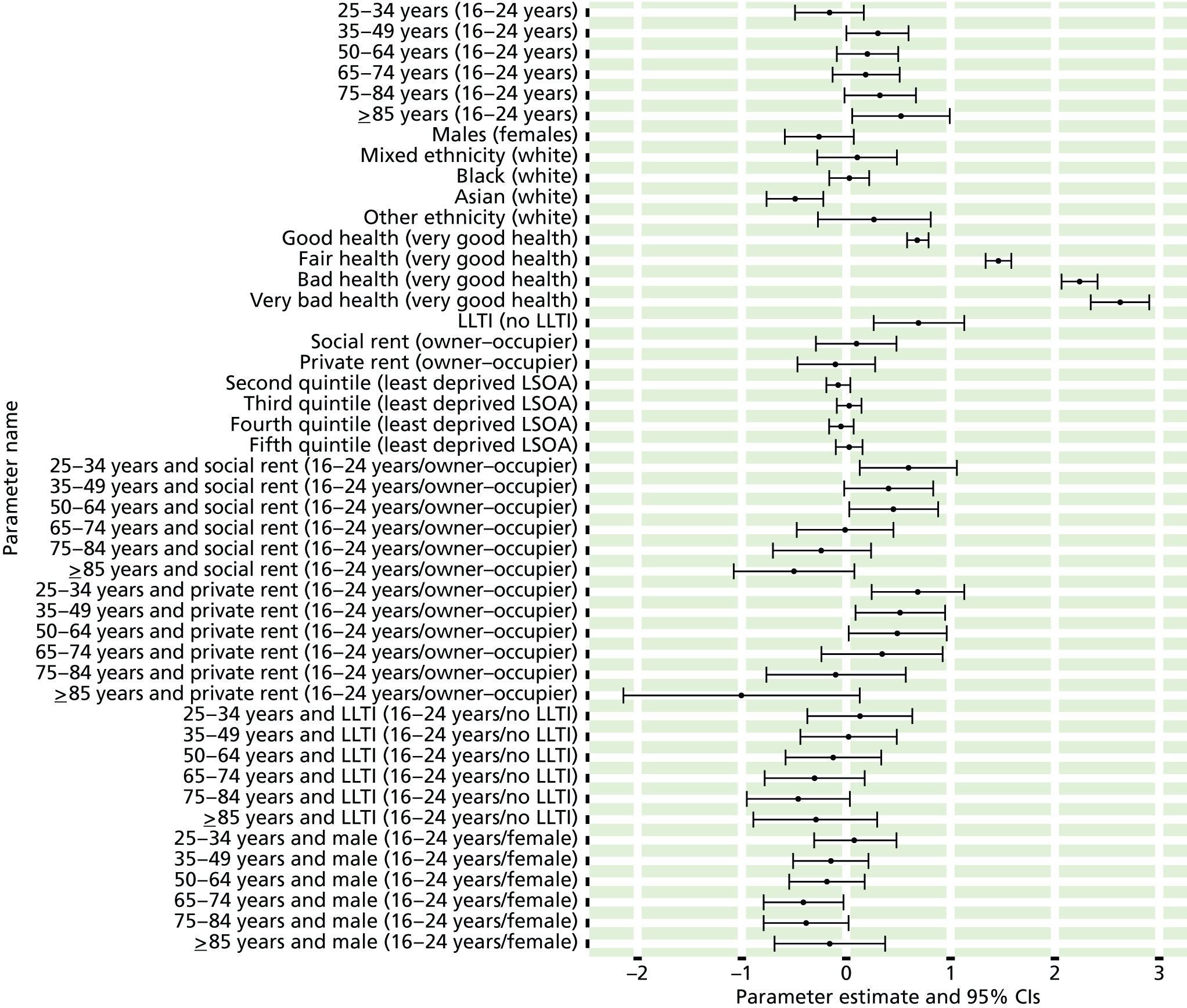
FIGURE 192.
Self-reported moderate/extreme anxiety/depression or anxiety/depression drugs: individual estimates and their 95% CIs. (a) MSOAs; (b) LAs; (c) CCGs; and (d) regions (GORs).
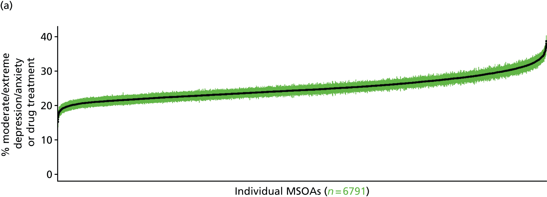
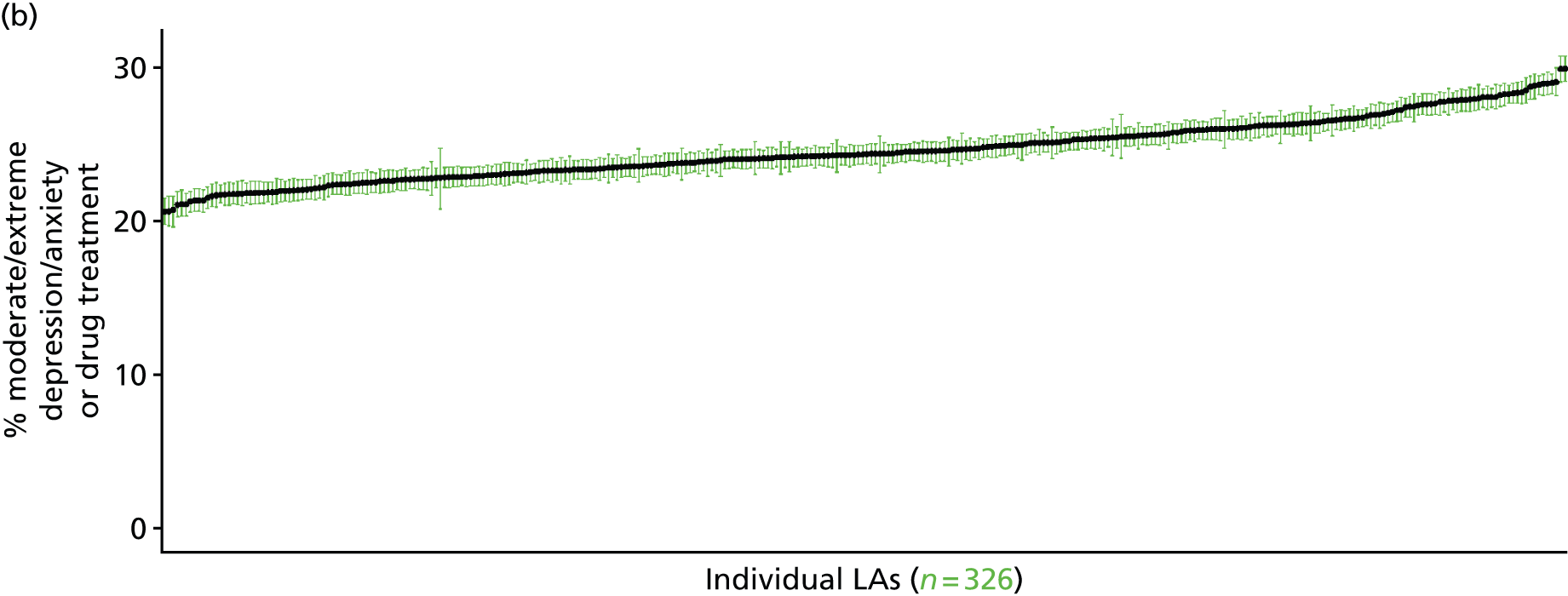
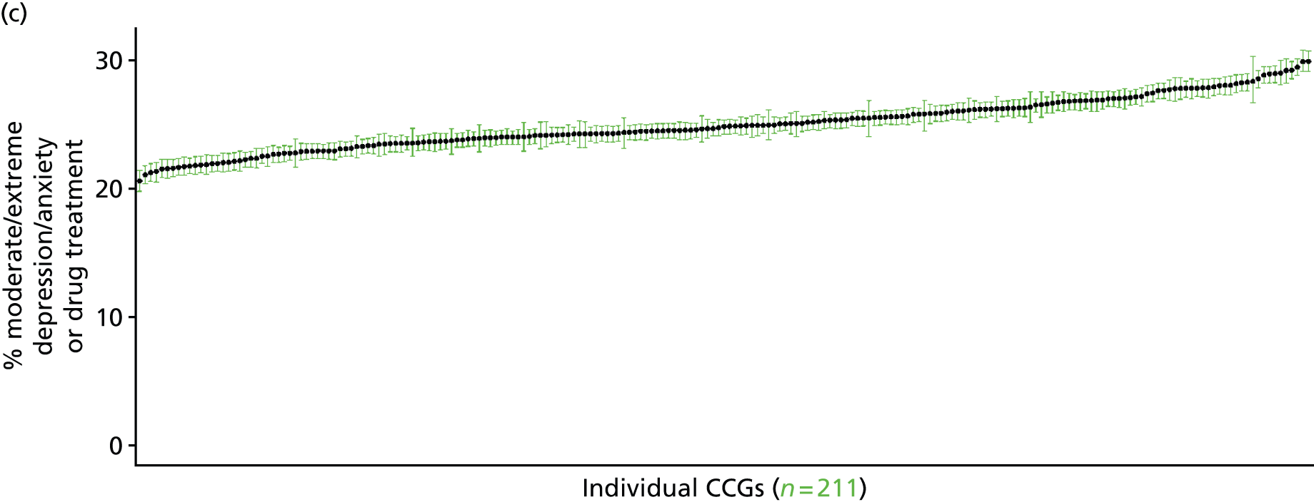

Self-reported extreme anxiety/depression or currently prescribed anxiety/depression drugs (Health Survey for England, 2006, 2008 and 2010–11)
FIGURE 193.
Self-reported extreme anxiety/depression or anxiety/depression drugs: LSOA-level map. Contains Ordnance Survey data © Crown copyright and database right 2012.
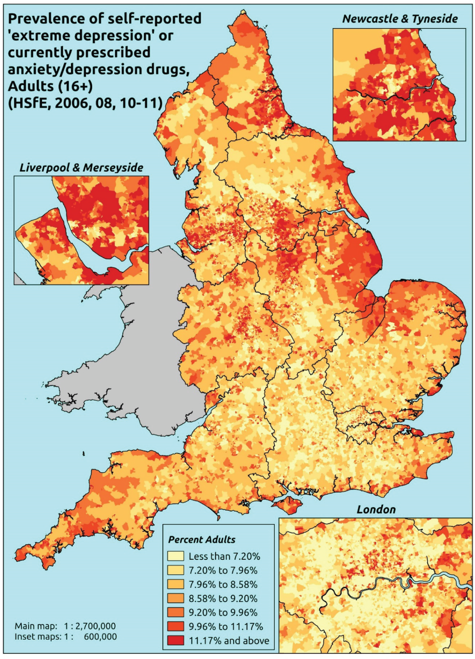
Response variable definition, provenance and prediction
Based on the recorded use of prescribed medication in addition to the EuroQol EQ-5D General Health instrument that was included in the HSfE in 2006, 2008 and 2010–11, respondents were asked to select one of the following options: (a) I am not anxious or depressed; (b) I am moderately anxious or depressed; or (c) I am extremely anxious or depressed. Here we capture those who have responded ‘yes’ to (c) or who are currently prescribed drugs for depression and/or anxiety (BNF 4.1.1–4.1.3 or 4.3.1–4.3.4487). This aims to capture individuals would have answered that they were extremely anxious or depressed because they are receiving medication. The problem, of course, is that here we will pick up individuals who would have been prescribed medication for moderate anxiety/depression, and thus this marker will overestimate levels of underlying ‘extreme’ anxiety/depression. There is no evidence available on whether or not they are receiving any other type of treatment. This marker of need is vulnerable to any sociodemographic or geographic variations in access to, or uptake of, care.
The HSfE at this time includes multiple household respondents of all ages. The analytical data set is drawn from a subset of respondents aged ≥ 16 years for whom data are available across all model response and predictor variables, namely whether or not they responded to this EuroQol EQ-5D question, whether or not data are available on current prescriptions, along with information on age band, sex, ethnicity, general health status, LLTI, tenure and the IMD quintile of the LSOA of residence (n = 31,018). A single randomly selected adult is then drawn from each household, resulting in an analytical data set of 18,301 adults aged ≥ 16 years.
| Age band (years) | Females | Age band (years) | Males | ||||
|---|---|---|---|---|---|---|---|
| Does not have condition | Has condition | % | Does not have condition | Has condition | % | ||
| 16–24 | 722 | 25 | 3.3 | 16–24 | 499 | 5 | 1.0 |
| 25–34 | 1434 | 119 | 7.7 | 25–34 | 942 | 42 | 4.3 |
| 35–49 | 2544 | 345 | 11.9 | 35–49 | 1921 | 119 | 5.8 |
| 50–64 | 2350 | 362 | 13.3 | 50–64 | 1923 | 183 | 8.7 |
| 65–74 | 1204 | 186 | 13.4 | 65–74 | 1059 | 92 | 8.0 |
| 75–84 | 868 | 154 | 15.1 | 75–84 | 628 | 48 | 7.1 |
| ≥ 85 | 288 | 54 | 15.8 | ≥ 85 | 164 | 21 | 11.4 |
| Females | 9410 | 1245 | 11.7 | Males | 7136 | 510 | 6.7 |
| Total (males and females) | 16,546 | 1755 | 9.6 | ||||
Model parameters are applied to microsimulated LSOA-level census data to produce estimates of the number (and proportion) of people expected to report extreme anxiety and/or depression or who are currently being prescribed drugs for depression and/or anxiety (BNF 4.1.1–4.1.3 or 4.3.1–4.3.4487) in each age–sex cohort (and overall) in each of the 32,844 English LSOAs. As discussed in the report, bootstrapping is used to derive 95% CIs for the estimates. These LSOA-level prevalence rate estimates (and 95% CIs) are aggregated into a number of higher geographies, namely MSOAs, LAs, CCGs and regions (GORs). Proportionate attribution is used to restructure the prevalence rate estimates to align with 2001 MSOAs, as well as GP practice populations as defined by the 2011 NHS ADS.
Table 215 summarises how expected prevalence rates vary by age, sex and local deprivation (as measured by the 2010 IMD). There are 6569 LSOAs (with 9,226,227 adults) classified as being in the least deprived quintile; 6568 LSOAs (9,525,344 adults) in the second least deprived quintile; 6568 LSOAs (9,658,444 adults) in the third least deprived quintile; 6568 LSOAs (9,650,576 adults) in the fourth least deprived quintile; and 6568 LSOAs (9,535,167 adults) in the most deprived quintile. Note that, as a general rule, variations in prevalence rates reflect variations in the socioeconomic composition of populations in the different types of LSOA rather than variations in deprivation per se.
| Cohort | Least deprived quintile LSOAs | Second least deprived quintile LSOAs | Third least deprived quintile LSOAs | Fourth least deprived quintile LSOAs | Most deprived quintile LSOAs | All England |
|---|---|---|---|---|---|---|
| Female 16–24 | 2.5 (1.7 to 3.5) | 2.2 (1.4 to 3.1) | 2.4 (1.6 to 3.2) | 2.3 (1.6 to 3.0) | 2.7 (1.8 to 3.5) | 2.4 (1.7 to 3.2) |
| Female 25–34 | 5.2 (4.4 to 6.2) | 4.8 (4.1 to 5.7) | 5.5 (4.7 to 6.3) | 5.7 (4.9 to 6.4) | 7.2 (6.2 to 8.1) | 5.8 (5.1 to 6.5) |
| Female 35–49 | 9.6 (8.4 to 10.5) | 9.3 (8.4 to 10.4) | 11.2 (10.1 to 12.2) | 12.0 (10.8 to 13.0) | 15.5 (13.6 to 16.7) | 11.5 (10.7 to 12.2) |
| Female 50–64 | 12.4 (11.3 to 13.7) | 12.3 (11.1 to 13.7) | 14.7 (13.5 to 16.1) | 16.3 (15.0 to 17.6) | 21.3 (19.1 to 23.0) | 15.1 (14.2 to 16.1) |
| Female 65–74 | 14.1 (12.7 to 15.9) | 13.6 (12.1 to 15.6) | 15.6 (13.9 to 17.3) | 16.2 (14.5 to 18.5) | 19.7 (17.6 to 22.7) | 15.6 (14.3 to 17.4) |
| Female ≥ 75 | 19.1 (16.7 to 21.0) | 17.4 (15.3 to 19.8) | 19.0 (16.3 to 21.2) | 18.1 (16.0 to 20.7) | 19.8 (16.9 to 22.3) | 18.6 (16.6 to 20.6) |
| Females | 11.0 (9.7 to 12.3) | 10.4 (9.2 to 11.8) | 11.7 (10.4 to 13.0) | 11.6 (10.3 to 12.9) | 13.9 (12.1 to 15.3) | 11.7 (10.7 to 12.8) |
| Male 16–24 | 1.1 (0.7 to 1.5) | 1.0 (0.7 to 1.4) | 1.1 (0.8 to 1.5) | 1.1 (0.8 to 1.5) | 1.5 (1.0 to 2.0) | 1.2 (0.8 to 1.6) |
| Male 25–34 | 2.5 (2.1 to 3.0) | 2.4 (2.0 to 2.9) | 2.8 (2.4 to 3.3) | 3.1 (2.6 to 3.6) | 4.5 (3.7 to 5.1) | 3.2 (2.7 to 3.6) |
| Male 35–49 | 4.4 (3.9 to 4.9) | 4.5 (4.0 to 5.1) | 5.8 (5.0 to 6.5) | 6.6 (5.7 to 7.4) | 9.5 (8.2 to 10.6) | 6.2 (5.6 to 6.7) |
| Male 50–64 | 6.3 (5.6 to 7.2) | 6.6 (5.8 to 7.4) | 8.4 (7.5 to 9.4) | 9.8 (8.8 to 10.9) | 14.0 (12.6 to 15.3) | 8.8 (8.2 to 9.5) |
| Male 65–74 | 7.6 (6.8 to 9.0) | 7.4 (6.6 to 8.8) | 9.0 (7.9 to 10.4) | 9.6 (8.5 to 11.6) | 12.5 (10.8 to 14.4) | 9.0 (8.1 to 10.3) |
| Male ≥ 75 | 10.1 (8.5 to 11.7) | 9.2 (8.0 to 10.8) | 10.2 (8.7 to 11.9) | 10.0 (8.5 to 12.0) | 11.4 (9.6 to 13.7) | 10.1 (8.8 to 11.7) |
| Males | 5.4 (4.7 to 6.2) | 5.2 (4.6 to 6.1) | 6.2 (5.3 to 7.0) | 6.4 (5.6 to 7.4) | 8.5 (7.4 to 9.6) | 6.3 (5.7 to 7.1) |
| All | 8.3 (7.6 to 8.9) | 7.9 (7.4 to 8.7) | 9.0 (8.3 to 9.7) | 9.1 (8.4 to 9.8) | 11.3 (10.3 to 12.0) | 9.1 (8.8 to 9.4) |
| Factor (reference group) | Model coefficients | 95% CI | ||
|---|---|---|---|---|
| Estimate | Standard error | 2.5% CI | 97.50% | |
| (Intercept) | –4.38152 | 0.3483 | –5.06418 | –3.69886 |
| Age (16–24 years) | ||||
| 25–34 years | 0.58146 | 0.37304 | –0.14970 | 1.31263 |
| 35–49 years | 1.17971 | 0.34553 | 0.50247 | 1.85696 |
| 50–64 years | 1.11331 | 0.34603 | 0.43509 | 1.79153 |
| 65–74 years | 1.27780 | 0.35440 | 0.58318 | 1.97243 |
| 75–84 years | 1.58266 | 0.36123 | 0.87465 | 2.29066 |
| ≥ 85 years | 1.89093 | 0.41161 | 1.08418 | 2.69769 |
| Sex (females) | ||||
| Males | –1.03266 | 0.10445 | –1.23739 | –0.82794 |
| Ethnicity (white) | ||||
| Mixed | –0.53974 | 0.37780 | –1.28023 | 0.20074 |
| Black | –0.76690 | 0.23181 | –1.22125 | –0.31256 |
| Asian | –0.79977 | 0.28152 | –1.35155 | –0.24799 |
| Other | –1.50919 | 1.04268 | –3.55285 | 0.53447 |
| General health status (very good) | ||||
| Good health | 0.74735 | 0.10667 | 0.53828 | 0.95643 |
| Fair health | 1.54514 | 0.12499 | 1.30016 | 1.79013 |
| Bad health | 2.81559 | 0.23646 | 2.35213 | 3.27906 |
| Very bad health | 2.99189 | 0.58551 | 1.84429 | 4.13949 |
| LLTI (no LTTI) | ||||
| LLTI | 1.17926 | 0.46327 | 0.27126 | 2.08726 |
| Tenure (owner–occupier) | ||||
| Social rent | 0.34248 | 0.44355 | –0.52689 | 1.21184 |
| Private rent or other tenure | –0.19424 | 0.50045 | –1.17511 | 0.78663 |
| LSOA deprivation quintile (least deprived quintile) | ||||
| Second quintile | –0.16484 | 0.08802 | –0.33735 | 0.00768 |
| Third quintile | –0.09180 | 0.08662 | –0.26157 | 0.07797 |
| Fourth quintile | –0.18701 | 0.09006 | –0.36353 | –0.01049 |
| Fifth quintile ( = most deprived quintile) | –0.12155 | 0.09256 | –0.30297 | 0.05987 |
| Interaction effects | ||||
| 25–34 years and LLTI (16–24 years/no LLTI) | 0.10368 | 0.43812 | –0.75504 | 0.96240 |
| 35–49 years and LLTI (16–24 years/no LLTI) | –0.24095 | 0.41402 | –1.05243 | 0.57053 |
| 50–64 years and LLTI (16–24 years/no LLTI) | –0.32910 | 0.41334 | –1.13924 | 0.48104 |
| 65–74 years and LLTI (16–24 years/no LLTI) | –0.68726 | 0.42386 | –1.51803 | 0.14350 |
| 75–84 years and LLTI (16–24 years/no LLTI) | –1.17761 | 0.43139 | –2.02313 | –0.33208 |
| ≥ 85 years and LLTI (16–24 years/no LLTI) | –1.25070 | 0.48478 | –2.20086 | –0.30054 |
| 25–34 years and social rent (16–24 years/owner–occupier) | 0.39106 | 0.49096 | –0.57122 | 1.35333 |
| 35–49 years and social rent (16–24 years/owner–occupier) | 0.17378 | 0.45968 | –0.72719 | 1.07475 |
| 50–64 years and social rent (16–24 years/owner–occupier) | –0.00972 | 0.45811 | –0.90761 | 0.88817 |
| 65–74 years and social rent (16–24 years/owner–occupier) | –0.31994 | 0.47161 | –1.24430 | 0.60443 |
| 75–84 years and social rent (16–24 years/owner–occupier) | –0.56243 | 0.47781 | –1.49894 | 0.37408 |
| ≥ 85 years and social rent (16–24 years/owner–occupier) | –0.97606 | 0.53275 | –2.02025 | 0.06813 |
| 25–34 years and private rent (16–24 years/owner–occupier) | 0.74691 | 0.54402 | –0.31938 | 1.81320 |
| 35–49 years and private rent (16–24 years/owner–occupier) | 0.69327 | 0.52295 | –0.33171 | 1.71824 |
| 50–64 years and private rent (16–24 years/owner–occupier) | 0.77457 | 0.53215 | –0.26846 | 1.81759 |
| 65–74 years and private rent (16–24 years/owner–occupier) | 0.23286 | 0.58882 | –0.92122 | 1.38694 |
| 75–84 years and private rent (16–24 years/owner–occupier) | –0.03171 | 0.63747 | –1.28116 | 1.21774 |
| ≥ 85 years and private rent (16–24 years/owner–occupier) | –0.32670 | 0.82406 | –1.94186 | 1.28845 |
| Male and LLTI (female/no LLTI) | 0.32475 | 0.12409 | 0.08152 | 0.56797 |
| Good health and LLTI (very good health/no LLTI) | 0.10680 | 0.26249 | –0.40767 | 0.62127 |
| Fair health and LLTI (very good health/no LLTI) | –0.08419 | 0.26411 | –0.60184 | 0.43346 |
| Bad health and LLTI (very good health/no LLTI) | –0.71388 | 0.33408 | –1.36868 | –0.05908 |
| Very bad health and LLTI (very good health/no LLTI) | –0.33156 | 0.63924 | –1.58448 | 0.92135 |
| Male and social rent (female/owner–occupier) | 0.28414 | 0.13860 | 0.01250 | 0.55579 |
| Male and private rent (female/owner–occupier) | 0.09122 | 0.18933 | –0.27986 | 0.46230 |
| Male and mixed (female/white) | 0.51708 | 0.73034 | –0.91438 | 1.94854 |
| Male and black (female/white) | 0.46737 | 0.35697 | –0.23230 | 1.16704 |
| Male and Asian (female/white) | –1.56020 | 1.05067 | –3.61952 | 0.49913 |
| Male and other (female/white) | 2.24701 | 1.21302 | –0.13051 | 4.62454 |
FIGURE 194.
Parameter plots: self-reported extreme anxiety/depression or anxiety/depression drugs.
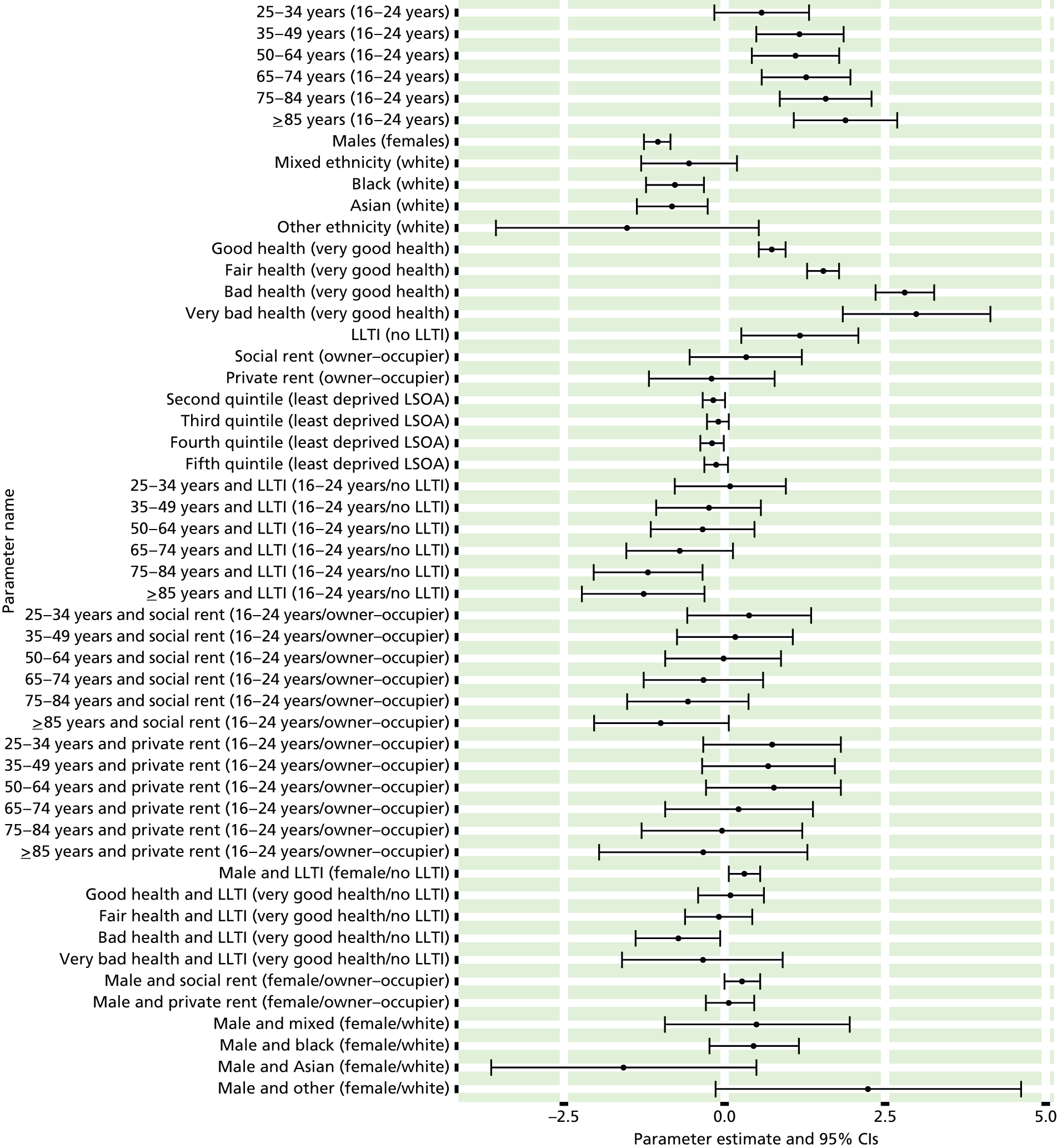
FIGURE 195.
Self-reported extreme anxiety/depression or anxiety/depression drugs: individual estimates and their 95% CIs. (a) MSOAs; (b) LAs; (c) CCGs; and (d) regions (GORs).


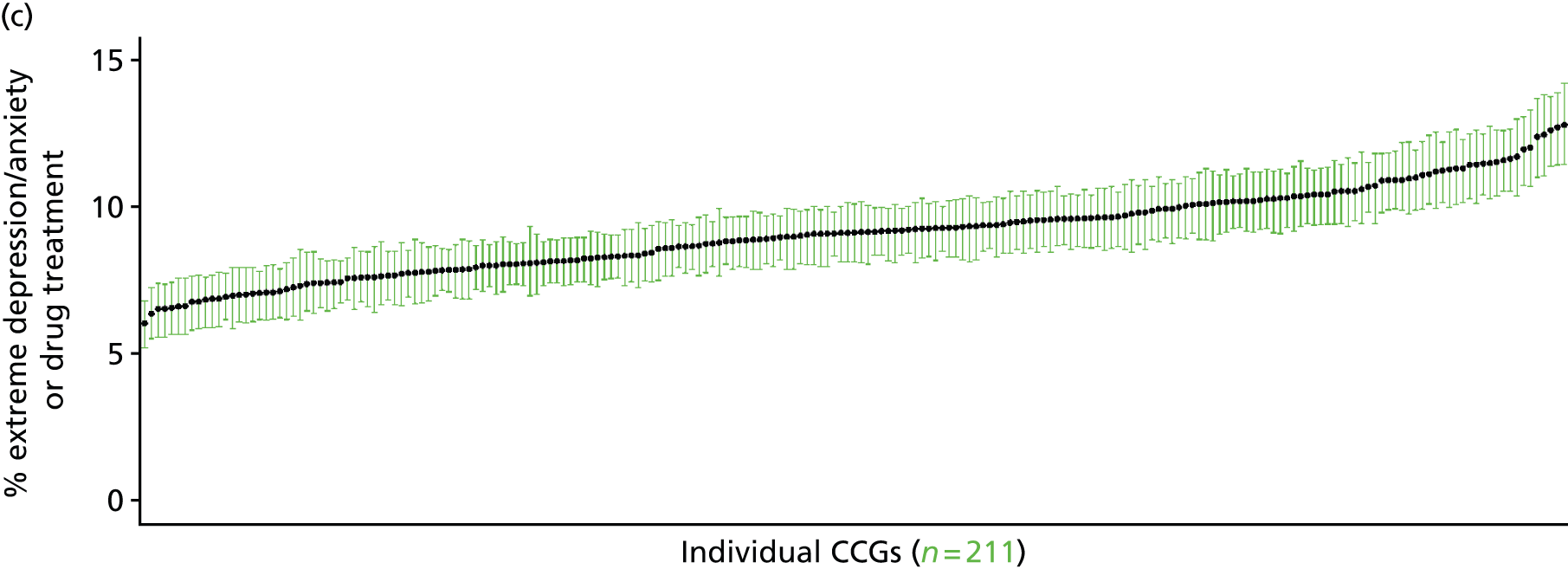
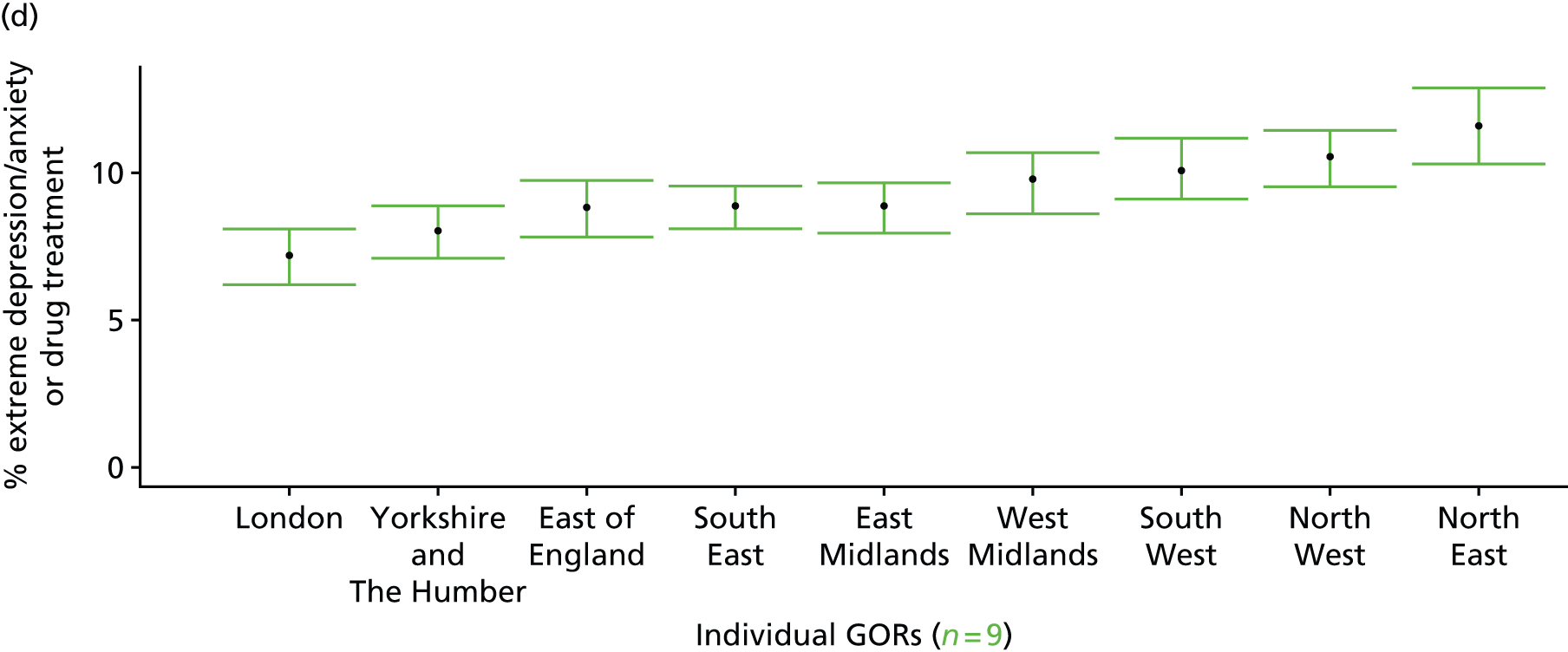
Self-reported ‘ever had a mental health issue’ (Adult Psychiatric Morbidity Survey, 2007)
FIGURE 196.
Self-reported ‘ever had a mental health issue’: LSOA-level map. Contains Ordnance Survey data © Crown copyright and database right 2012.
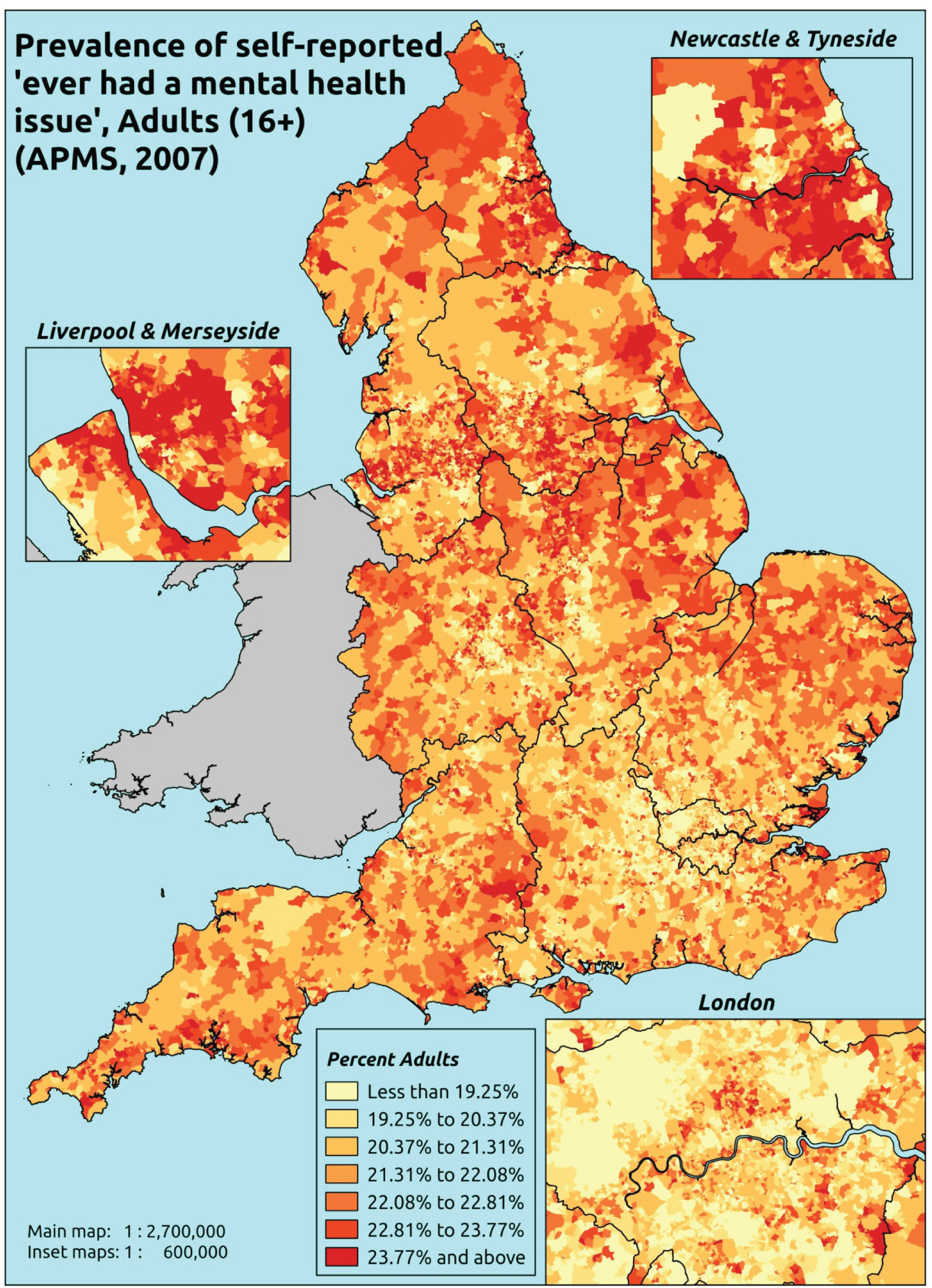
Response variable definition, provenance and prediction
Respondents to the APMS were asked whether or not they had any of a series of conditions since the age of 16 years, including ‘anxiety, depression or other mental health issue’. Unlike the three APMS variables above, addressing mental health issues experienced during the previous 12 months, this does not specify that they should say yes ‘even if you have not experienced any symptoms because you use medication or an aid’. This is, however, unlikely to be an issue as, unlike the previous APMS questions, this question is not given a time frame. This, of course, is not so much a marker of ‘need for mental health-care services’ as a measure of the proportion of people who have been affected by mental health issues at some point in their adult life – although one might expect this to be strongly correlated with need for care services.
Although this does not specify that the ‘mental health issue’ needs to have been specifically doctor diagnosed, this measure will still be influenced by access to, and use of, health-care services; this is in part because individuals are presumably more likely to report a mental health issue if they have been diagnosed with such, and in part because somatisation means that many mental health conditions initially present as physical symptoms, and individuals will recognise that they have a ‘mental health issue’ only once it has been identified as such by a GP or other health professional.
The APMS data set (n = 7403) comprises adults aged ≥ 16 years (living in England) and surveyed only one person per household; thus, the analytical data set contains all respondents for whom data are available across all model response and predictor variables, namely CIS-R score, age band, sex, ethnicity, LLTI, tenure and IMD quintile of LSOA of residence (n = 7323).
| Age band (years) | Females | Age band (years) | Males | ||||
|---|---|---|---|---|---|---|---|
| Does not have condition | Has condition | % | Does not have condition | Has condition | % | ||
| 16–24 | 236 | 57 | 19.5 | 16–24 | 243 | 23 | 8.6 |
| 25–34 | 432 | 182 | 29.6 | 25–34 | 335 | 72 | 17.7 |
| 35–49 | 740 | 376 | 33.7 | 35–49 | 683 | 188 | 21.6 |
| 50–64 | 681 | 332 | 32.8 | 50–64 | 655 | 142 | 17.8 |
| 65–74 | 422 | 139 | 24.8 | 65–74 | 403 | 57 | 12.4 |
| 75–84 | 368 | 67 | 15.4 | 75–84 | 255 | 30 | 10.5 |
| ≥ 85 | 112 | 21 | 15.8 | ≥ 85 | 63 | 9 | 12.5 |
| Females | 2991 | 1174 | 28.2 | Males | 2637 | 521 | 16.5 |
| Total (males and females) | 5628 | 1695 | 23.1 | ||||
Model parameters are applied to microsimulated LSOA-level census data to produce estimates of the number (and proportion) of people who have ever had a mental health issue in each age–sex cohort (and overall) in each of the 32,844 English LSOAs. As discussed in the report, bootstrapping is used to derive 95% CIs for the estimates. These LSOA-level prevalence rate estimates (and 95% CIs) are aggregated into a number of higher geographies, namely MSOAs, LAs, CCGs and regions (GORs). Proportionate attribution is used to restructure the prevalence rate estimates to align with 2001 MSOAs, as well as GP practice populations as defined by the 2011 NHS ADS.
Table 218 summarises how expected prevalence rates vary by age, sex and local deprivation (as measured by the 2010 IMD). There are 6569 LSOAs (with 9,226,227 adults) classified as being in the least deprived quintile; 6568 LSOAs (9,525,344 adults) in the second least deprived quintile; 6568 LSOAs (9,658,444 adults) in the third least deprived quintile; 6568 LSOAs (9,650,576 adults) in the fourth least deprived quintile; and 6568 LSOAs (9,535,167 adults) in the most deprived quintile. Note that, as a general rule, variations in prevalence rates reflect variations in the socioeconomic composition of populations in the different types of LSOA rather than variations in deprivation per se.
| Cohort | Least deprived quintile LSOAs | Second least deprived quintile LSOAs | Third least deprived quintile LSOAs | Fourth least deprived quintile LSOAs | Most deprived quintile LSOAs | All England |
|---|---|---|---|---|---|---|
| Female 16–24 | 16.3 (12.6 to 19.4) | 17.8 (14.5 to 21.4) | 17.6 (14.3 to 21.3) | 15.8 (12.3 to 18.6) | 16.5 (13.2 to 19.8) | 16.7 (13.4 to 19.7) |
| Female 25–34 | 26.7 (22.5 to 30.2) | 28.9 (25.1 to 32.5) | 28.6 (24.6 to 31.6) | 26.1 (22.7 to 29.2) | 27.4 (24.0 to 31.1) | 27.5 (24.4 to 30.1) |
| Female 35–49 | 30.5 (27.7 to 33.6) | 33.7 (31.0 to 36.7) | 34.1 (31.3 to 37.0) | 32.5 (29.1 to 35.3) | 35.2 (31.5 to 38.6) | 33.2 (31.0 to 35.5) |
| Female 50–64 | 28.7 (25.6 to 31.5) | 32.0 (29.3 to 35.0) | 32.5 (29.7 to 35.7) | 31.2 (27.6 to 34.0) | 34.5 (31.3 to 38.4) | 31.7 (29.6 to 33.7) |
| Female 65–74 | 22.3 (19.3 to 25.2) | 25.1 (22.1 to 27.9) | 25.4 (22.1 to 29.1) | 24.1 (20.1 to 26.8) | 26.2 (22.8 to 30.0) | 24.5 (21.8 to 27.1) |
| Female ≥ 75 | 16.3 (13.3 to 19.3) | 18.1 (15.4 to 20.9) | 18.1 (15.0 to 21.1) | 16.6 (13.2 to 19.0) | 17.5 (14.4 to 21.5) | 17.3 (14.8 to 19.8) |
| Females | 25.2 (22.0 to 28.2) | 27.7 (24.7 to 30.8) | 27.7 (24.6 to 30.9) | 26.0 (22.5 to 28.8) | 27.9 (24.5 to 31.5) | 26.9 (24.3 to 29.3) |
| Male 16–24 | 8.7 (6.6 to 10.7) | 9.7 (7.7 to 12.2) | 9.6 (7.5 to 12.0) | 8.7 (6.7 to 10.7) | 9.7 (7.3–12.0) | 9.3 (7.3 to 11.3) |
| Male 25–34 | 15.1 (12.4 to 17.8) | 16.6 (14.4 to 19.1) | 16.6 (13.6 to 18.7) | 15.2 (12.7 to 17.5) | 16.7 (14.4 to 19.4) | 16.1 (14.0 to 18.1) |
| Male 35–49 | 17.4 (15.7 to 19.6) | 19.8 (17.6 to 22.5) | 20.4 (18.4 to 22.8) | 19.7 (17.1 to 21.6) | 22.7 (20.3 to 25.4) | 20.0 (18.5 to 21.8) |
| Male 50–64 | 16.1 (14.2 to 18.5) | 18.5 (16.5 to 20.8) | 19.1 (16.9 to 21.5) | 18.6 (16.2 to 21.2) | 21.7 (19.5 to 24.8) | 18.7 (17.1 to 20.5) |
| Male 65–74 | 12.0 (10.1 to 14.0) | 13.9 (11.7 to 16.3) | 14.3 (12.2 to 16.5) | 13.8 (11.1 to 15.8) | 15.8 (13.3 to 18.4) | 13.9 (12.0 to 15.7) |
| Male ≥ 75 | 8.3 (6.7 to 10.3) | 9.4 (7.8 to 11.5) | 9.6 (7.8 to 11.6) | 8.8 (6.9 to 10.3) | 9.7 (7.7 to 12.0) | 9.1 (7.5 to 10.7) |
| Males | 14.1 (12.2 to 16.3) | 15.9 (13.9 to 18.4) | 16.3 (14.0 to 18.6) | 15.5 (13.1 to 17.6) | 17.6 (15.3 to 20.3) | 15.9 (14.1 to 17.7) |
| All | 19.8 (17.9 to 21.6) | 22.0 (20.2 to 23.6) | 22.2 (20.7 to 23.9) | 20.9 (18.9 to 22.4) | 22.9 (21.1 to 24.7) | 21.6 (20.7 to 22.3) |
| Factor (reference group) | Model coefficients | 95% CI | ||
|---|---|---|---|---|
| Estimate | SE | 2.5% CI | 97.50% | |
| (Intercept) | –1.86456 | 0.16303 | –2.18410 | –1.54502 |
| Age (16–24 years) | ||||
| 25–34 years | 0.69887 | 0.16601 | 0.37349 | 1.02425 |
| 35–49 years | 0.81609 | 0.15700 | 0.50837 | 1.12381 |
| 50–64 years | 0.63722 | 0.16385 | 0.31607 | 0.95836 |
| 65–74 years | 0.13799 | 0.19455 | –0.24332 | 0.51931 |
| 75–84 years | –0.35353 | 0.26269 | –0.86842 | 0.16135 |
| ≥ 85 years | –0.17576 | 0.49551 | –1.14696 | 0.79545 |
| Sex (females) | ||||
| Males | –0.76074 | 0.07577 | –0.90926 | –0.61222 |
| Ethnicity (white) | ||||
| Mixed | 0.39582 | 0.29784 | –0.18794 | 0.97957 |
| Black | –0.86151 | 0.20301 | –1.25941 | –0.46361 |
| Asian | –0.70151 | 0.21056 | –1.11420 | –0.28881 |
| Other | –1.13537 | 0.49610 | –2.10773 | –0.16301 |
| LLTI (no LTTI) | ||||
| LLTI | 1.58179 | 0.31519 | 0.96401 | 2.19957 |
| Tenure (owner–occupier) | ||||
| Social rent | 0.21547 | 0.09676 | 0.02583 | 0.40511 |
| Private rent or other tenure | 0.33644 | 0.12101 | 0.09926 | 0.57363 |
| LSOA deprivation quintile (least deprived quintile) | ||||
| Second quintile | 0.10396 | 0.09246 | –0.07725 | 0.28517 |
| Third quintile | 0.07976 | 0.09532 | –0.10706 | 0.26659 |
| Fourth quintile | –0.05889 | 0.09842 | –0.25179 | 0.13401 |
| Fifth quintile ( = most deprived quintile) | –0.02319 | 0.10107 | –0.22129 | 0.17490 |
| Interaction effects | ||||
| 25–34 years and LLTI (16–24 years/no LLTI) | –0.20380 | 0.36496 | –0.91912 | 0.51152 |
| 35–49 years and LLTI (16–24 years/no LLTI) | –0.11992 | 0.33627 | –0.77901 | 0.53917 |
| 50–64 years and LLTI (16–24 years/no LLTI) | –0.52149 | 0.33429 | –1.17670 | 0.13373 |
| 65–74 years and LLTI (16–24 years/no LLTI) | –0.65828 | 0.35651 | –1.35704 | 0.04049 |
| 75–84 years and LLTI (16–24 years/no LLTI) | –0.85698 | 0.40452 | –1.64984 | –0.06412 |
| ≥ 85 years and LLTI (16–24 years/no LLTI) | –1.13189 | 0.61043 | –2.32834 | 0.06456 |
| Male and social rent (female/owner–occupier) | 0.35195 | 0.15326 | 0.05155 | 0.65235 |
| Male and private rent (female/owner–occupier) | –0.15301 | 0.19703 | –0.53920 | 0.23318 |
FIGURE 197.
Parameter plots: self-reported ‘ever had a mental health issue’.
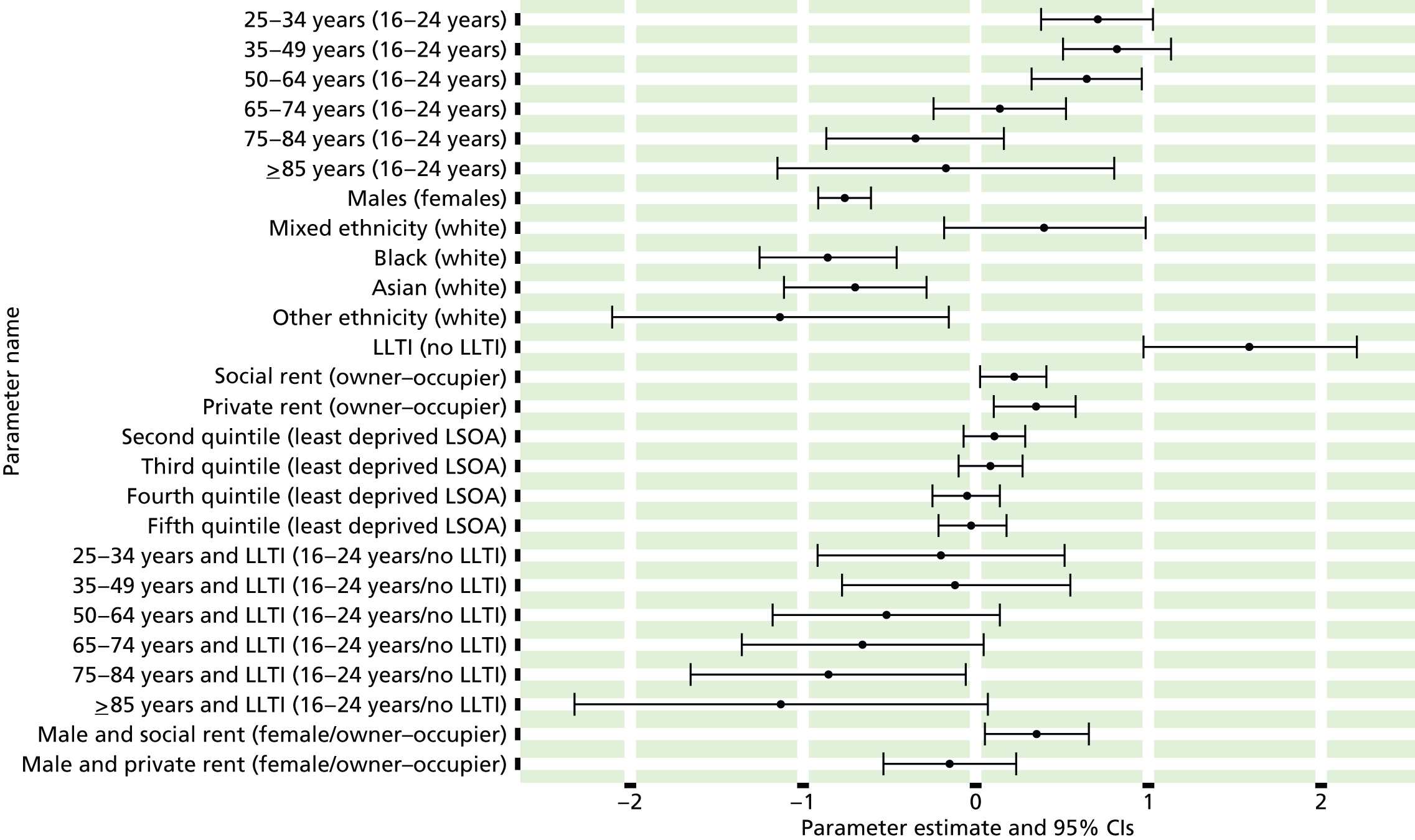
FIGURE 198.
Self-reported ‘ever had a mental health issue’: individual estimates and their 95% CIs. (a) MSOAs; (b) LAs; (c) CCGs; and (d) regions (GORs). MH, mental health.
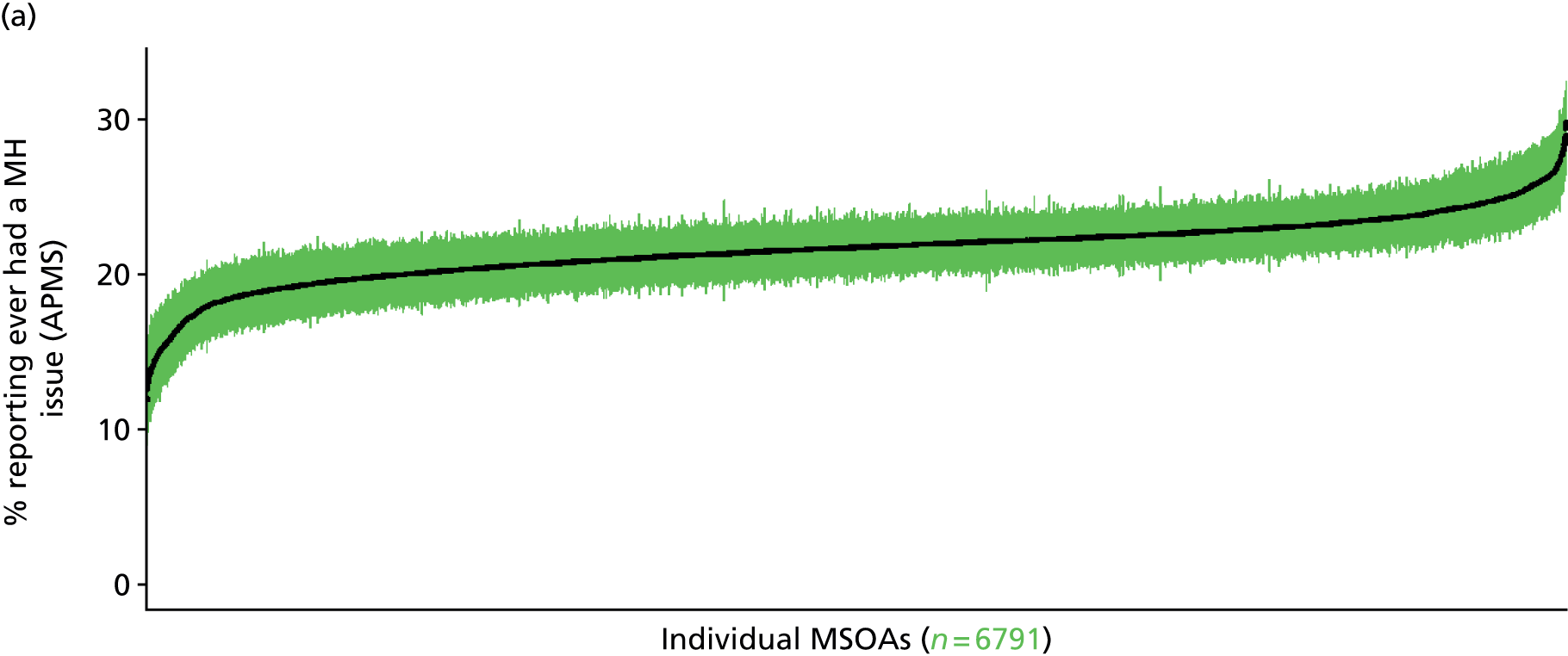
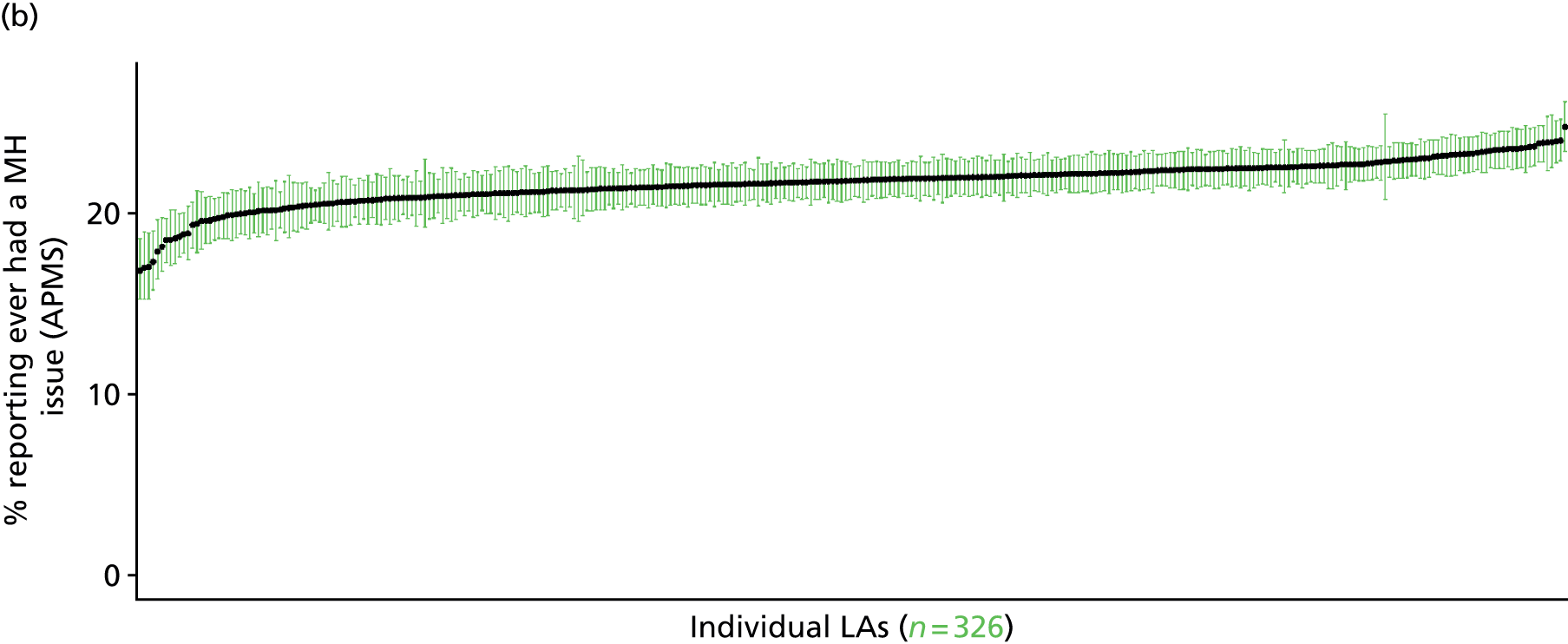
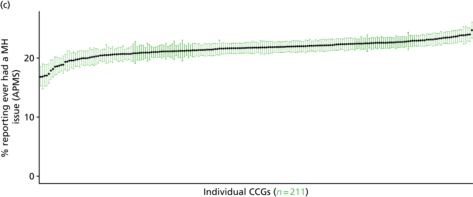
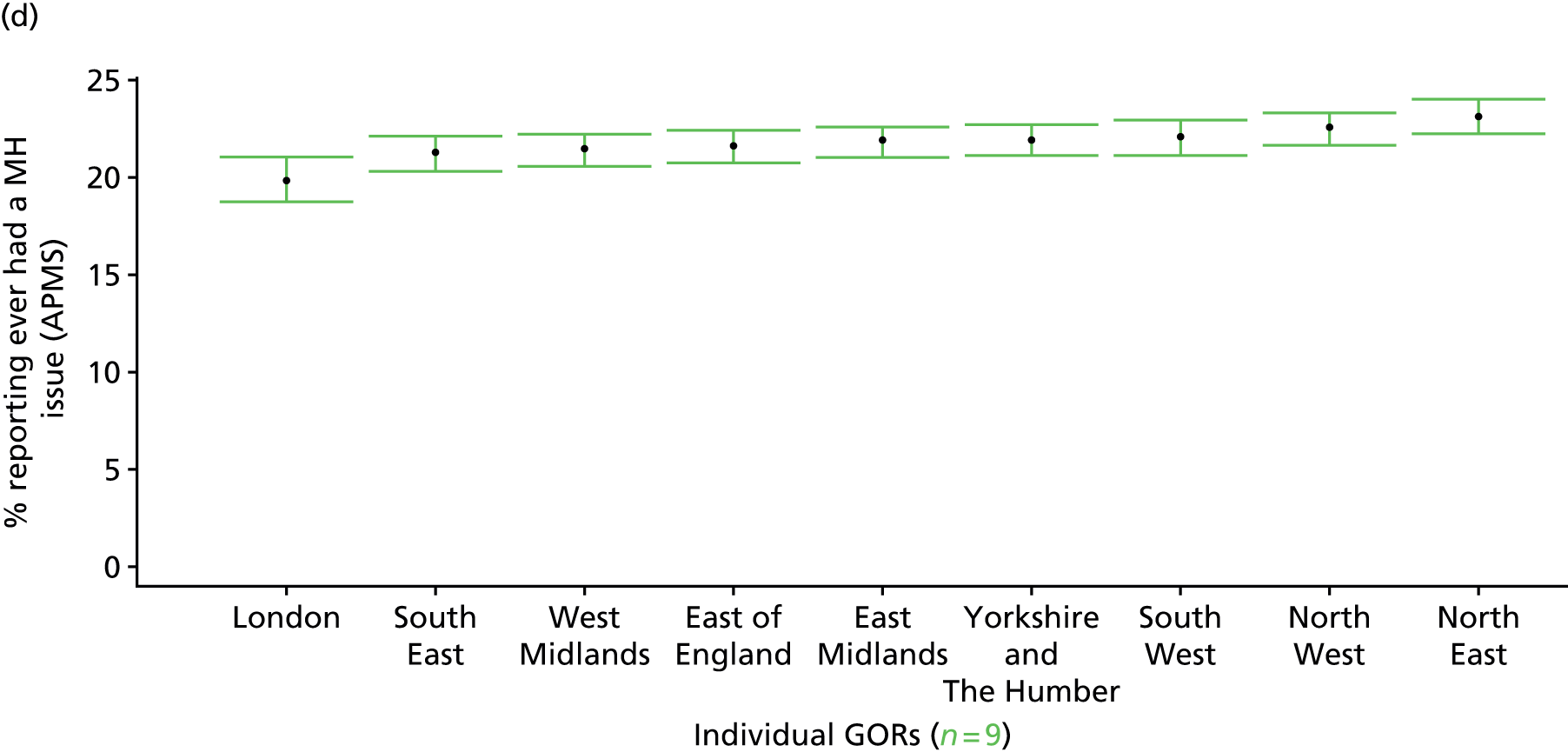
Self-reported ‘mental health issue’ in last 12 months (Adult Psychiatric Morbidity Survey, 2007)
FIGURE 199.
Self-reported ‘mental health issue’ in last 12 months: LSOA-level map. Contains Ordnance Survey data © Crown copyright and database right 2012.
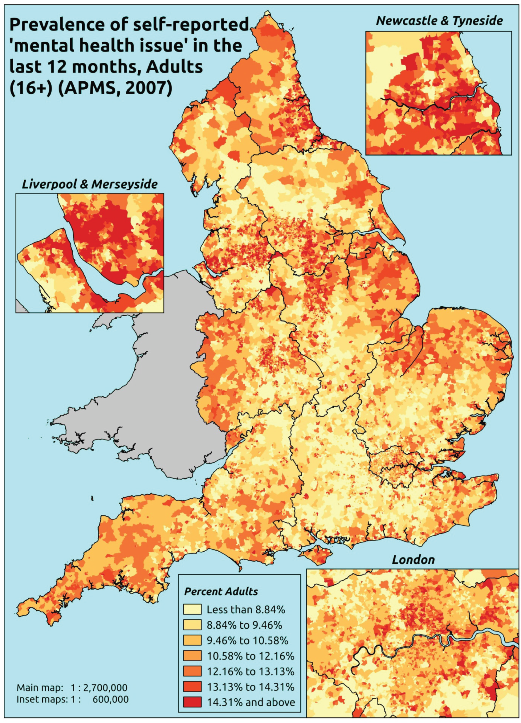
Response variable definition, provenance and prediction
Respondents to the APMS who have said that they have had any ‘anxiety, depression or other mental health issue’ since the age of 16 years were then asked whether or not they had had the condition in the past 12 months, and directed to say yes ‘even if you have not experienced any symptoms because you use medication or an aid’ [our emphasis]. This addresses the issue discussed at length in the previous section, and thus this measure is likely to be a much more reliable marker of ‘need for health care’ than simply the presence of a self-reported long-standing mental health problem. Note, however, that this question does not specify how long the condition has been present, and so it is not entirely comparable (see below for a more direct comparator). Although possibly less affected by sociodemographic and/or geographic variations in access to, or uptake of, mental health care than most measures, this will nevertheless be influenced by access to, and use of, primary services, as somatisation means that many mental health conditions initially present as physical symptoms, and individuals will recognise that they have a ‘mental health issue’ only once it has been identified as such by a GP or another health professional.
The APMS data set (n = 7403) comprises adults ≥ 16 years (living in England) and surveyed only one person per household, and thus the analytical data set contains all respondents for whom data are available across all model response and predictor variables, namely CIS-R score, age band, sex, ethnicity, LLTI, tenure and IMD quintile of LSOA of residence (n = 7323).
| Age band (years) | Females | Age band (years) | Males | ||||
|---|---|---|---|---|---|---|---|
| Does not have condition | Has condition | % | Does not have condition | Has condition | % | ||
| 16–24 | 254 | 39 | 13.3 | 16–24 | 251 | 15 | 5.6 |
| 25–34 | 517 | 97 | 15.8 | 25–34 | 370 | 37 | 9.1 |
| 35–49 | 900 | 216 | 19.4 | 35–49 | 769 | 102 | 11.7 |
| 50–64 | 836 | 177 | 17.5 | 50–64 | 733 | 64 | 8.0 |
| 65–74 | 485 | 76 | 13.5 | 65–74 | 438 | 22 | 4.8 |
| 75–84 | 398 | 37 | 8.5 | 75–84 | 270 | 15 | 5.3 |
| ≥ 85 | 125 | 8 | 6.0 | ≥ 85 | 65 | 7 | 9.7 |
| Females | 3515 | 650 | 15.6 | Males | 2896 | 262 | 8.3 |
| Total (males and females) | 6411 | 912 | 12.5 | ||||
Model parameters are applied to microsimulated LSOA-level census data to produce estimates of the number (and proportion) of people expected to have had a mental health issue in the last 12 months in each age–sex cohort (and overall) in each of the 32,844 English LSOAs. As discussed in the report, bootstrapping is used to derive 95% CIs for the estimates. These LSOA-level prevalence rate estimates (and 95% CIs) are aggregated into a number of higher geographies, namely MSOAs, LAs, CCGs and regions (GORs). Proportionate attribution is used to restructure the prevalence rate estimates to align with 2001 MSOAs, as well as GP practice populations as defined by the 2011 NHS ADS.
Table 221 summarises how expected prevalence rates vary by age, sex and local deprivation (as measured by the 2010 IMD). There are 6569 LSOAs (with 9,226,227 adults) classified as being in the least deprived quintile; 6568 LSOAs (9,525,344 adults) in the second least deprived quintile; 6568 LSOAs (9,658,444 adults) in the third least deprived quintile; 6568 LSOAs (9,650,576 adults) in the fourth least deprived quintile; and 6568 LSOAs (9,535,167 adults) in the most deprived quintile. Note that, as a general rule, variations in prevalence rates reflect variations in the socioeconomic composition of populations in the different types of LSOA rather than variations in deprivation per se.
| Cohort | Least deprived quintile LSOAs | Second least deprived quintile LSOAs | Third least deprived quintile LSOAs | Fourth least deprived quintile LSOAs | Most deprived quintile LSOAs | All England |
|---|---|---|---|---|---|---|
| Female 16–24 | 10.0 (7.6 to 12.8) | 10.0 (7.9 to 12.9) | 13.2 (10.6 to 16.5) | 11.3 (8.5 to 14.3) | 12.5 (9.8 to 15.6) | 11.5 (9.2 to 14.3) |
| Female 25–34 | 12.2 (9.7 to 14.5) | 12.2 (9.7 to 15.0) | 16.0 (13.1 to 19.1) | 14.1 (11.6 to 16.6) | 16.0 (13.3 to 18.9) | 14.4 (12.1 to 16.5) |
| Female 35–49 | 15.1 (12.7 to 17.2) | 15.8 (13.8 to 18.7) | 21.1 (18.6 to 24.0) | 19.5 (17.0 to 22.1) | 23.1 (20.5 to 25.8) | 18.9 (17.5 to 20.8) |
| Female 50–64 | 12.3 (10.2 to 14.0) | 13.2 (11.3 to 15.5) | 18.4 (15.9 to 21.5) | 17.8 (15.4 to 20.5) | 22.5 (19.5 to 25.4) | 16.6 (14.8 to 18.5) |
| Female 65–74 | 9.7 (7.3 to 11.8) | 10.4 (8.4 to 12.7) | 14.7 (11.8 to 17.3) | 14.0 (10.1 to 16.1) | 17.3 (13.5 to 20.7) | 12.9 (10.4 to 15.2) |
| Female ≥ 75 | 7.8 (5.9 to 9.9) | 8.1 (6.2 to 10.5) | 11.4 (9.0 to 14.4) | 10.2 (7.5 to 12.5) | 11.9 (9.0 to 15.3) | 9.8 (7.7 to 12.0) |
| Females | 11.9 (9.6 to 13.9) | 12.3 (10.3 to 14.9) | 16.7 (14.1 to 19.7) | 15.3 (12.6 to 17.9) | 18.2 (15.4 to 21.2) | 14.9 (13.0 to 17.0) |
| Male 16–24 | 4.9 (3.5 to 6.3) | 5.0 (3.8 to 6.5) | 6.8 (5.4 to 9.0) | 6.1 (4.4 to 7.9) | 7.3 (5.7 to 9.4) | 6.1 (4.9 to 7.7) |
| Male 25–34 | 6.0 (4.5 to 7.4) | 6.1 (4.7 to 7.9) | 8.3 (6.8 to 10.4) | 7.6 (5.9 to 9.1) | 9.3 (7.4 to 11.3) | 7.7 (6.4 to 9.2) |
| Male 35–49 | 7.4 (5.7 to 8.7) | 7.8 (6.4 to 9.6) | 11.2 (9.7 to 13.4) | 10.7 (8.8 to 12.4) | 14.0 (11.8 to 16.4) | 10.2 (8.9 to 11.8) |
| Male 50–64 | 5.9 (4.7 to 6.9) | 6.5 (5.3 to 7.8) | 9.6 (8.4 to 11.6) | 9.6 (8.1 to 11.4) | 13.2 (11.3 to 15.4) | 8.8 (7.8 to 10.1) |
| Male 65–74 | 4.6 (3.3 to 5.8) | 5.0 (3.9 to 6.2) | 7.5 (5.9 to 9.1) | 7.4 (5.5 to 9.1) | 9.9 (7.7 to 12.2) | 6.6 (5.4 to 8.0) |
| Male ≥ 75 | 3.6 (2.5 to 4.6) | 3.8 (2.8 to 5.0) | 5.5 (4.1 to 7.3) | 5.1 (3.7 to 6.5) | 6.5 (4.7 to 8.7) | 4.8 (3.6 to 6.0) |
| Males | 5.8 (4.4 to 7.0) | 6.1 (4.9 to 7.6) | 8.8 (7.4 to 10.8) | 8.4 (6.7 to 10.1) | 10.9 (8.9 to 13.1) | 8.0 (6.8 to 9.4) |
| All | 8.9 (7.5 to 10.0) | 9.3 (8.2 to 10.8) | 12.9 (11.6 to 14.7) | 12.0 (10.3 to 13.5) | 14.6 (13.0 to 16.4) | 11.6 (10.9 to 12.4) |
| Factor (reference group) | Model coefficients | 95% CI | ||
|---|---|---|---|---|
| Estimate | SE | 2.5% CI | 97.50% | |
| (Intercept) | –2.38568 | 0.18871 | –2.75556 | –2.01579 |
| Age (16–24 years) | ||||
| 25–34 years | 0.23602 | 0.18104 | –0.11881 | 0.59085 |
| 35–49 years | 0.41002 | 0.16815 | 0.08045 | 0.73959 |
| 50–64 years | –0.08679 | 0.17477 | –0.42933 | 0.25575 |
| 65–74 years | –0.69976 | 0.19489 | –1.08175 | –0.31777 |
| 75–84 years | –1.29323 | 0.21978 | –1.72400 | –0.86246 |
| ≥ 85 years | –1.49555 | 0.31857 | –2.11994 | –0.87115 |
| Sex (females) | ||||
| Males | –0.86436 | 0.10492 | –1.06999 | –0.65872 |
| Ethnicity (white) | ||||
| Mixed | 0.79588 | 0.38042 | 0.05025 | 1.54151 |
| Black | –0.78471 | 0.36836 | –1.50671 | –0.06272 |
| Asian | –1.27150 | 0.51498 | –2.28086 | –0.26215 |
| Other | 0.04608 | 0.61879 | –1.16674 | 1.25891 |
| LLTI (no LTTI) | ||||
| LLTI | 1.44479 | 0.10197 | 1.24493 | 1.64465 |
| Tenure (owner–occupier) | ||||
| Social rent | 0.03959 | 0.16677 | –0.28729 | 0.36647 |
| Private rent or other tenure | –0.09467 | 0.19333 | –0.47360 | 0.28426 |
| LSOA deprivation quintile (least deprived quintile) | ||||
| Second quintile | –0.01192 | 0.12922 | –0.26520 | 0.24136 |
| Third quintile | 0.32596 | 0.12485 | 0.08126 | 0.57067 |
| Fourth quintile | 0.14178 | 0.12930 | –0.11165 | 0.39521 |
| Fifth quintile ( = most deprived quintile) | 0.24202 | 0.13005 | –0.01288 | 0.49692 |
| Interaction effects | ||||
| Male and social rent (female/owner–occupier) | 0.54132 | 0.18738 | 0.17405 | 0.90859 |
| Male and private rent (female/owner–occupier) | –0.01901 | 0.26552 | –0.53942 | 0.50141 |
| LLTI and social rent (no LLTI/owner–occupier) | 0.32311 | 0.18870 | –0.04675 | 0.69296 |
| LLTI and private rent (no LLTI/owner–occupier) | 0.61669 | 0.25114 | 0.12446 | 1.10893 |
| Mixed and LLTI (white/no LLTI) | –0.16195 | 0.76671 | –1.66471 | 1.34081 |
| Black and LLTI (white/no LLTI) | 0.75725 | 0.48955 | –0.20226 | 1.71675 |
| Asian and LLTI (white/no LLTI) | 0.54326 | 0.62646 | –0.68460 | 1.77112 |
| Other and LLTI (white/no LLTI) | –12.8935 | 165.4733 | –337.221 | 311.4342 |
FIGURE 200.
Parameter plots: self-reported ‘mental health issue’ in last 12 months.
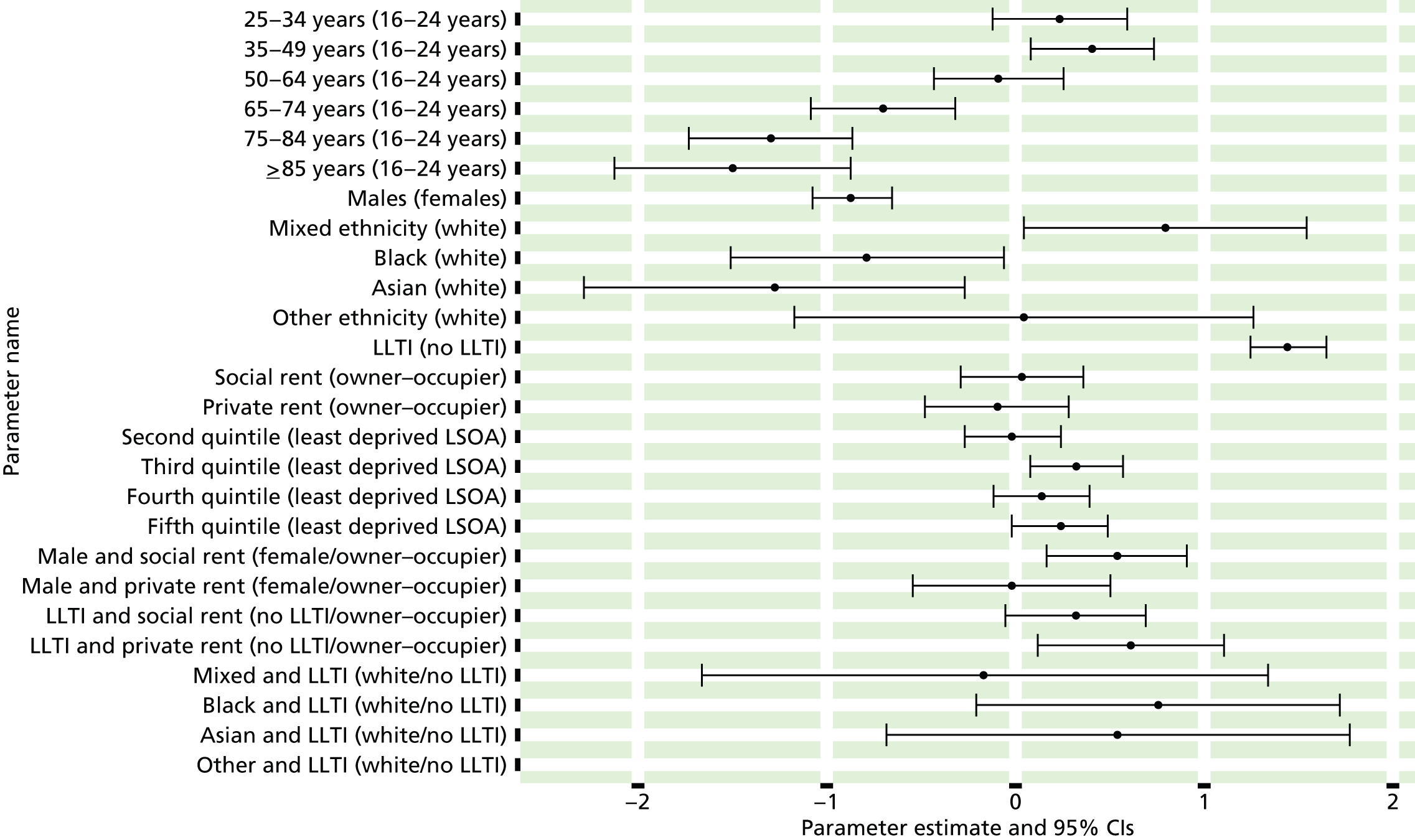
FIGURE 201.
Self-reported ‘mental health issue’ in last 12 months: individual estimates and their 95% CIs. (a) MSOAs; (b) LAs; (c) CCGs; and (d) regions (GORs). MH, mental health.
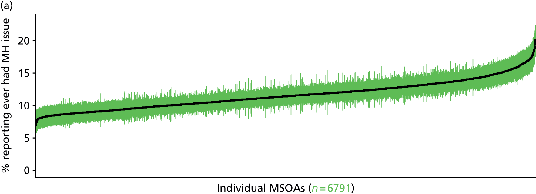

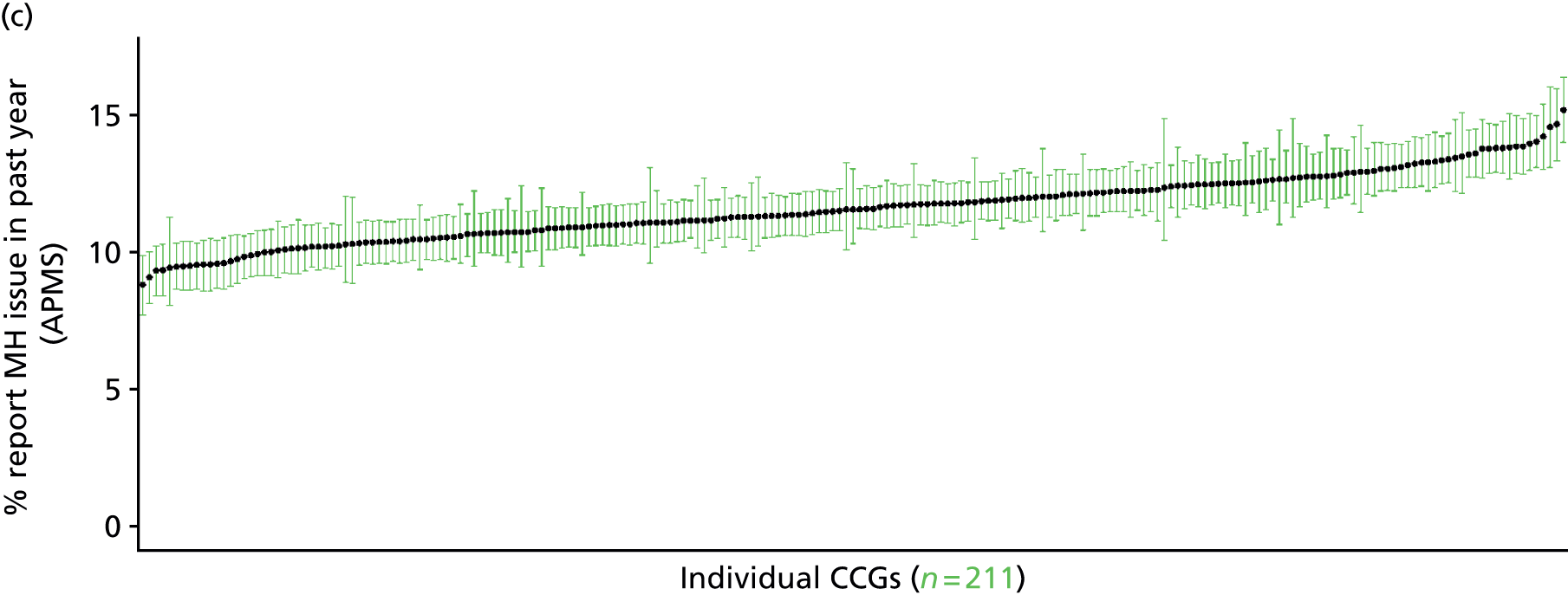
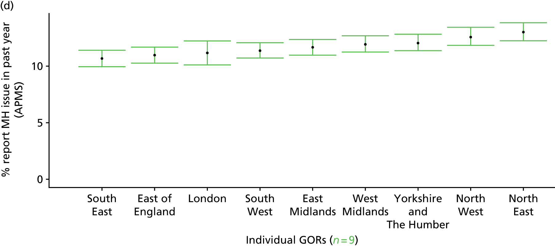
Self-reported ‘mental health issue’ in last 12 months first experienced at least 1 year previously (Adult Psychiatry Morbidity Survey, 2007)
FIGURE 202.
Self-reported ‘mental health issue’ in last 12 months first experienced > 1 year ago: LSOA-level map. Contains Ordnance Survey data © Crown copyright and database right 2012.
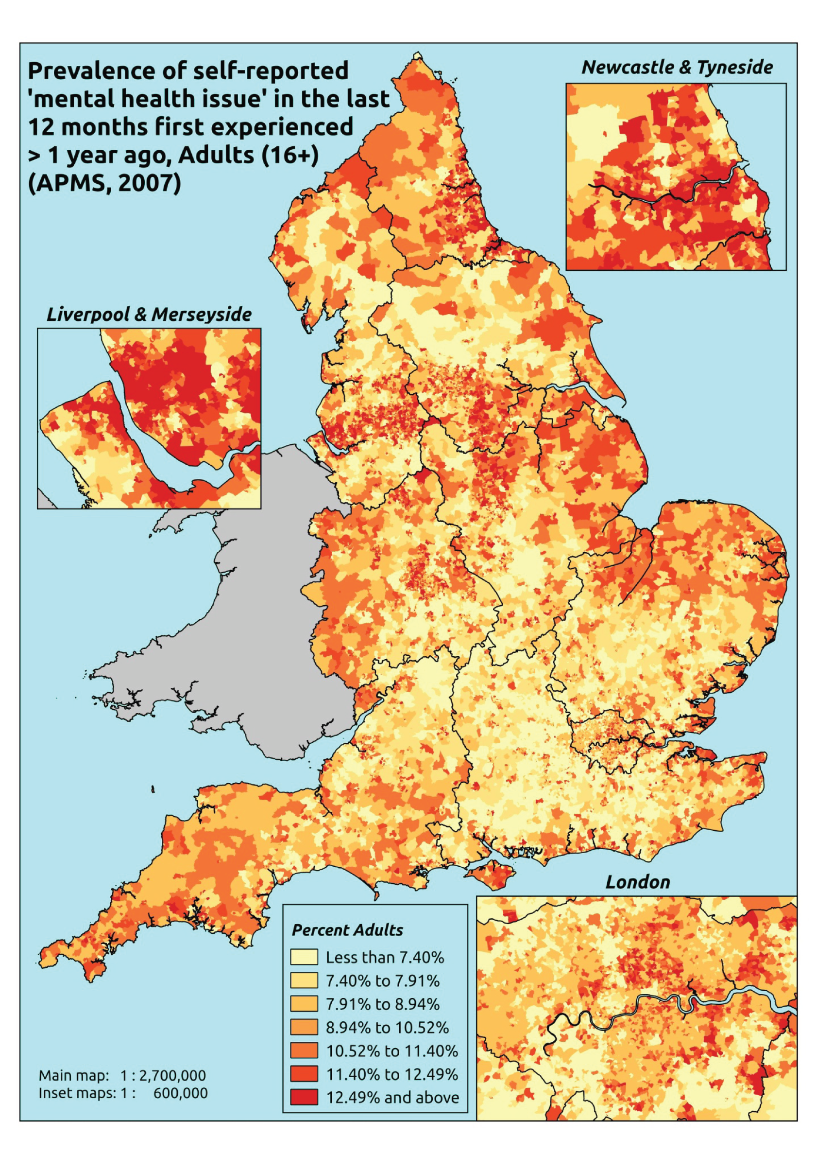
Response variable definition, provenance and prediction
Respondents to the APMS who state that they have had any ‘anxiety, depression or other mental health issue’ over the last 12 months are asked whether they first suffered from it over 1 year ago. Once again, it is explicitly stated that they should say yes ‘even if you have not experienced any symptoms because you use medication or an aid’. This gets closer to representing a ‘long-standing’ condition (although the wording means that a respondent could respond yes if they had a condition that lasted only, say, 4 months from 14 months to 10 months previously). Such notwithstanding, this appears a better measure of a long-standing mental health problem than the HSfE version, which does not explicitly draw attention to conditions controlled by drugs or other treatments. The difference between this measure (with an overall adult prevalence rate of 10.8%) and the HSfE self-reported long-standing mental health problem prevalence rate (of 4.4%) is possibly indicative of the impact of treatment on whether or not individuals are likely to view their condition as having ‘troubled’ them.
Although possibly less affected by sociodemographic and/or geographic variations in access to, or uptake of, mental health care than most measures, this will nevertheless be influenced by access to, and use of, primary services, as somatisation means that many mental health conditions initially present as physical symptoms, and individuals will only recognise that they have a ‘mental health issue’ once it has been identified as such by a GP or another health professional.
The APMS data set (n = 7403) comprises adults ≥ 16 (living in England) and surveyed only one person per household, and thus the analytical data set contains all respondents for whom data are available across all model response and predictor variables, namely CIS-R score, age band, sex, ethnicity, LLTI, tenure and IMD quintile of LSOA of residence (n = 7323).
| Age band (years) | Females | Age band (years) | Males | ||||
|---|---|---|---|---|---|---|---|
| Does not have condition | Has condition | % | Does not have condition | Has condition | % | ||
| 16–24 | 261 | 32 | 10.9 | 16–24 | 254 | 12 | 4.5 |
| 25–34 | 533 | 81 | 13.2 | 25–34 | 377 | 30 | 7.4 |
| 35–49 | 934 | 182 | 16.3 | 35–49 | 777 | 94 | 10.8 |
| 50–64 | 855 | 158 | 15.6 | 50–64 | 738 | 59 | 7.4 |
| 65–74 | 495 | 66 | 11.8 | 65–74 | 439 | 21 | 4.6 |
| 75–84 | 403 | 32 | 7.4 | 75–84 | 273 | 12 | 4.2 |
| ≥ 85 | 128 | 5 | 3.8 | ≥ 85 | 66 | 6 | 8.3 |
| Females | 3609 | 556 | 13.3 | Males | 2924 | 234 | 7.4 |
| Total (males and females) | 6533 | 790 | 10.8 | ||||
Model parameters are applied to microsimulated LSOA-level census data to produce estimates of the number (and proportion) of people expected to have had a mental health issue in the last 12 months which was first experienced over a year ago in each age–sex cohort (and overall) in each of the 32,844 English LSOAs. As discussed in the report, bootstrapping is used to derive 95% CIs for the estimates. These LSOA-level prevalence rate estimates (and 95% CIs) are aggregated into a number of higher geographies, namely MSOAs, LAs, CCGs and regions (GORs). Proportionate attribution is used to restructure the prevalence rate estimates to align with 2001 MSOAs, as well as GP practice populations as defined by the 2011 NHS ADS.
Table 224 summarises how expected prevalence rates vary by age, sex and local deprivation (as measured by the 2010 IMD). There are 6569 LSOAs (with 9,226,227 adults) classified as being in the least deprived quintile; 6568 LSOAs (9,525,344 adults) in the second least deprived quintile; 6568 LSOAs (9,658,444 adults) in the third least deprived quintile; 6568 LSOAs (9,650,576 adults) in the fourth least deprived quintile; and 6568 LSOAs (9,535,167 adults) in the most deprived quintile. Note that, as a general rule, variations in prevalence rates reflect variations in the socioeconomic composition of populations in the different types of LSOA rather than variations in deprivation per se.
| Cohort | Least deprived quintile LSOAs | Second least deprived quintile LSOAs | Third least deprived quintile LSOAs | Fourth least deprived quintile LSOAs | Most deprived quintile LSOAs | All England |
|---|---|---|---|---|---|---|
| Female 16–24 | 8.3 (5.9 to 12.1) | 8.3 (5.6 to 11.4) | 11.5 (8.3 to 15.5) | 9.8 (7.1 to 13.5) | 10.8 (7.8 to 14.8) | 9.9 (7.2 to 13.4) |
| Female 25–34 | 9.8 (7.4 to 12.4) | 9.8 (7.7 to 12.4) | 13.4 (10.9 to 16.7) | 11.7 (9.6 to 14.2) | 13.4 (11.0 to 16.4) | 11.9 (9.8 to 14.2) |
| Female 35–49 | 11.9 (9.9 to 14.9) | 12.4 (10.4 to 14.8) | 17.4 (14.9 to 20.3) | 16.1 (13.8 to 19.0) | 19.3 (17.0 to 22.5) | 15.4 (13.8 to 17.6) |
| Female 50–64 | 11.1 (9.1 to 13.5) | 11.8 (9.7 to 14.1) | 17.1 (14.3 to 20.2) | 16.6 (13.7 to 19.3) | 20.9 (17.9 to 24.4) | 15.2 (13.1 to 17.6) |
| Female 65–74 | 8.8 (6.2 to 11.3) | 9.4 (6.8 to 11.4) | 13.9 (10.7 to 16.7) | 13.1 (10.1 to 15.9) | 16.2 (12.4 to 19.9) | 12.0 (9.4 to 14.2) |
| Female ≥ 75 | 5.3 (3.3 to 7.2) | 5.4 (3.5 to 7.0) | 7.9 (5.4 to 10.3) | 7.0 (4.8 to 8.6) | 8.2 (5.6 to 11.0) | 6.7 (4.6 to 8.6) |
| Females | 9.8 (7.6 to 12.5) | 10.1 (8.0 to 12.4) | 14.3 (11.6 to 17.4) | 13.2 (10.6 to 15.9) | 15.7 (12.9 to 19.0) | 12.6 (10.5 to 15.0) |
| Male 16–24 | 3.2 (1.6 to 5.0) | 3.3 (1.6 to 5.1) | 4.8 (2.5 to 7.2) | 4.2 (2.2 to 6.2) | 5.2 (2.8 to 7.9) | 4.2 (2.2 to 6.2) |
| Male 25–34 | 4.5 (3.0 to 6.3) | 4.5 (3.0 to 6.4) | 6.5 (4.2 to 9.3) | 5.8 (3.8 to 7.9) | 7.3 (5.1 to 10.1) | 6.0 (4.0 to 8.1) |
| Male 35–49 | 6.9 (5.7 to 9.2) | 7.4 (5.7 to 9.4) | 11.0 (9.2 to 13.4) | 10.5 (8.5 to 12.4) | 13.8 (11.5 to 16.9) | 10.0 (8.4 to 11.8) |
| Male 50–64 | 4.7 (3.4 to 6.1) | 5.2 (3.8 to 6.5) | 8.1 (6.1 to 9.8) | 8.2 (6.1 to 10.0) | 11.3 (8.6 to 13.7) | 7.3 (5.7 to 8.8) |
| Male 65–74 | 3.4 (1.9 to 4.9) | 3.8 (2.1 to 5.3) | 5.9 (3.3 to 8.4) | 5.8 (3.5 to 8.1) | 7.8 (4.5 to 10.8) | 5.2 (3.0 to 7.0) |
| Male ≥ 75 | 4.6 (2.9 to 6.8) | 4.8 (2.8 to 7.5) | 7.1 (4.3 to 10.3) | 6.6 (3.9 to 9.6) | 8.1 (5.1 to 11.5) | 6.1 (3.7 to 8.8) |
| Males | 4.9 (3.5 to 6.8) | 5.2 (3.6 to 7.0) | 7.8 (5.6 to 10.2) | 7.4 (5.3 to 9.4) | 9.6 (7.1 to 12.4) | 7.0 (5.1 to 8.9) |
| All | 7.4 (6.3 to 8.9) | 7.8 (6.5 to 9.0) | 11.2 (9.7 to 12.4) | 10.4 (9.0 to 11.4) | 12.7 (11.3 to 14.3) | 9.9 (9.3 to 10.5) |
| Factor (reference group) | Model coefficients | 95% CI | ||
|---|---|---|---|---|
| Estimate | SE | 2.5% CI | 97.50% | |
| (Intercept) | –2.59699 | 0.23278 | –3.05324 | –2.14073 |
| Age (16–24 years) | ||||
| 25–34 years | 0.17544 | 0.23531 | –0.28576 | 0.63664 |
| 35–49 years | 0.29708 | 0.21984 | –0.13380 | 0.72797 |
| 50–64 years | –0.05439 | 0.22575 | –0.49686 | 0.38809 |
| 65–74 years | –0.66610 | 0.24793 | –1.15205 | –0.18015 |
| 75–84 years | –1.43499 | 0.28043 | –1.98463 | –0.88535 |
| ≥ 85 years | –2.37380 | 0.50399 | –3.36162 | –1.38598 |
| Sex (females) | ||||
| Males | –1.08677 | 0.38109 | –1.83371 | –0.33983 |
| Ethnicity (white) | ||||
| Mixed | 0.62252 | 0.36925 | –0.10121 | 1.34624 |
| Black | –0.38898 | 0.24988 | –0.87874 | 0.10078 |
| Asian | –0.82749 | 0.29855 | –1.41266 | –0.24232 |
| Other | –1.91437 | 1.03052 | –3.93418 | 0.10544 |
| LLTI (no LTTI) | ||||
| LLTI | 1.54562 | 0.10689 | 1.33611 | 1.75513 |
| Tenure (owner–occupier) | ||||
| Social rent | –0.07567 | 0.1869 | –0.44199 | 0.29065 |
| Private rent or other tenure | –0.09106 | 0.2128 | –0.50816 | 0.32603 |
| LSOA deprivation quintile (least deprived quintile) | ||||
| Second quintile | –0.01877 | 0.13969 | –0.29256 | 0.25503 |
| Third quintile | 0.35788 | 0.13371 | 0.09581 | 0.61994 |
| Fourth quintile | 0.16900 | 0.13862 | –0.10271 | 0.44070 |
| Fifth quintile ( = most deprived quintile) | 0.26538 | 0.13903 | –0.00712 | 0.53788 |
| Interaction effects | ||||
| LLTI and social rent (no LLTI/owner–occupier) | 0.45305 | 0.20597 | 0.04934 | 0.85675 |
| LLTI and private rent (no LLTI/owner–occupier) | 0.65368 | 0.26659 | 0.13116 | 1.17620 |
| Male and social rent (female/owner–occupier) | 0.56772 | 0.19858 | 0.17850 | 0.95693 |
| Male and private rent (female/owner–occupier) | –0.02797 | 0.28986 | –0.59610 | 0.54017 |
| 25–34 years and male (16–24 years/female) | 0.16070 | 0.43479 | –0.69149 | 1.01290 |
| 35–49 years and male (16–24 years/female) | 0.46049 | 0.39553 | –0.31475 | 1.23572 |
| 50–64 years and male (16–24 years/female) | 0.10807 | 0.40556 | –0.68682 | 0.90296 |
| 65–74 years and male (16–24 years/female) | 0.01093 | 0.45489 | –0.88065 | 0.90251 |
| 75–84 years and male (16–24 years/female) | 0.43998 | 0.51072 | –0.56103 | 1.44100 |
| ≥ 85 years and male (16–24 years female) | 2.07077 | 0.73329 | 0.63353 | 3.50801 |
FIGURE 203.
Parameter plots: self-reported ‘mental health issue’ in last 12 months first experienced > 1 year ago.

FIGURE 204.
Self-reported ‘mental health issue’ in last 12 months first experienced > 1 year ago: individual estimates and their 95% CIs. (a) MSOAs; (b) LAs; (c) CCGs; and (d) regions (GORs). MH, mental health.

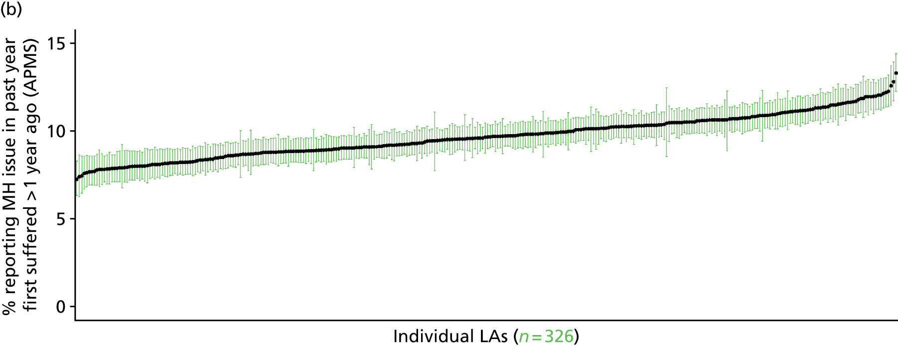

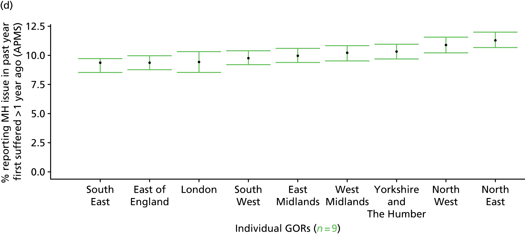
Self-reported ‘mental health issue’ in last 12 months first experienced at least 5 years previously (Adult Psychiatry Morbidity Survey, 2007)
FIGURE 205.
Self-reported ‘mental health issue’ in last 12 months first experienced > 5 years ago: LSOA-level map. Contains Ordnance Survey data © Crown copyright and database right 2012.
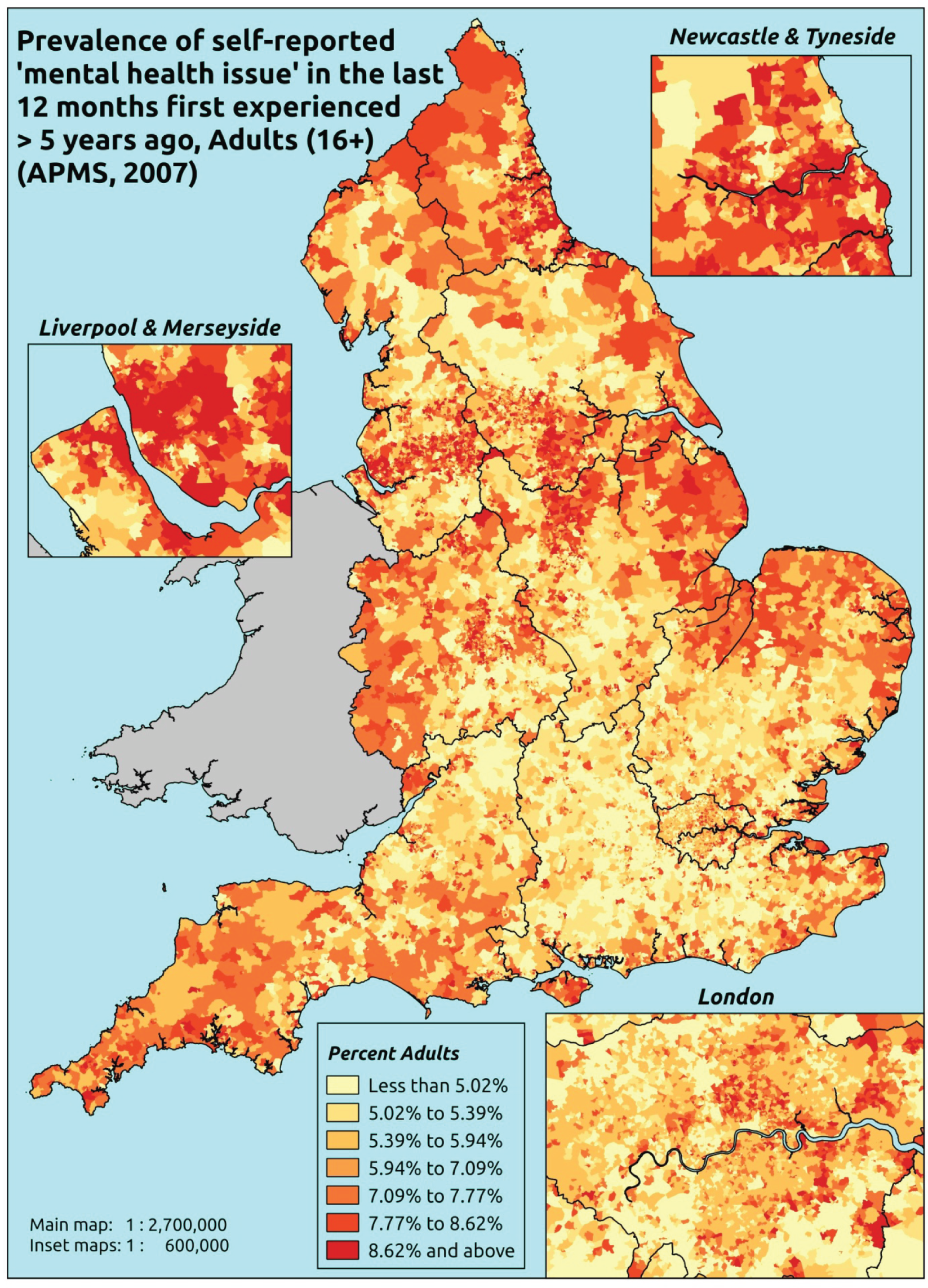
Response variable definition, provenance and prediction
Respondents to the APMS who stated that they have had any ‘anxiety, depression or other mental health issue’ over the last 12 months were asked whether they first suffered from it over 5 years ago. Once again, it is explicitly stated that they should say yes ‘even if you have not experienced any symptoms because you use medication or an aid’. This undoubtedly represents a ‘long-standing’ condition. Indeed, it might be interpreted as providing the basis for a measure of long-term, ongoing and unresolved mental health problems. Once again, although possibly less affected by sociodemographic and/or geographic variations in access to, or uptake of, mental health care than most measures, this will nevertheless be influenced by access to, and use of, primary services, as somatisation means many mental health conditions initially present as physical symptoms, and individuals will recognise that they have a ‘mental health issue’ only once it has been identified as such by a GP or another health professional.
The APMS data set (n = 7403) comprises adults ≥ 16 years (living in England) and surveyed only one person per household, and thus the analytical data set contains all respondents for whom data are available across all model response and predictor variables, namely CIS-R score, age band, sex, ethnicity, LLTI, tenure and IMD quintile of LSOA of residence (n = 7323).
| Age band (years) | Females | Age band (years) | Males | ||||
|---|---|---|---|---|---|---|---|
| Does not have condition | Has condition | % | Does not have condition | Has condition | % | ||
| 16–24 | 282 | 11 | 3.8 | 16–24 | 263 | 3 | 1.1 |
| 25–34 | 563 | 51 | 8.3 | 25–34 | 387 | 20 | 4.9 |
| 35–49 | 981 | 135 | 12.1 | 35–49 | 804 | 67 | 7.7 |
| 50–64 | 888 | 125 | 12.3 | 50–64 | 758 | 39 | 4.9 |
| 65–74 | 510 | 51 | 9.1 | 65–74 | 442 | 18 | 3.9 |
| 75–84 | 414 | 21 | 4.8 | 75–84 | 279 | 6 | 2.1 |
| ≥ 85 | 131 | 2 | 1.5 | ≥ 85 | 68 | 4 | 5.6 |
| Females | 3769 | 396 | 9.5 | Males | 3001 | 157 | 5.0 |
| Total (males and females) | 6770 | 553 | 7.6 | ||||
Model parameters are applied to microsimulated LSOA-level census data to produce estimates of the number (and proportion) of people expected to have a long-term, ongoing and unresolved mental health issue in each age–sex cohort (and overall) in each of the 32,844 English LSOAs. As discussed in the report, bootstrapping is used to derive 95% CIs for the estimates. These LSOA-level prevalence rate estimates (and 95% CIs) are aggregated into a number of higher geographies, namely MSOAs, LAs, CCGs, and regions (GORs). Proportionate attribution is used to restructure the prevalence rate estimates to align with 2001 MSOAs, as well as GP practice populations as defined by the 2011 NHS ADS.
Table 227 summarises how expected prevalence rates vary by age, sex and local deprivation (as measured by the 2010 IMD). There are 6569 LSOAs (with 9,226,227 adults) classified as being in the least deprived quintile; 6568 LSOAs (9,525,344 adults) in the second least deprived quintile; 6568 LSOAs (9,658,444 adults) in the third least deprived quintile; 6568 LSOAs (9,650,576 adults) in the fourth least deprived quintile; and 6568 LSOAs (9,535,167 adults) in the most deprived quintile. Note that, as a general rule, variations in prevalence rates reflect variations in the socioeconomic composition of populations in the different types of LSOA rather than variations in deprivation per se.
| Cohort | Least deprived quintile LSOAs | Second least deprived quintile LSOAs | Third least deprived quintile LSOAs | Fourth least deprived quintile LSOAs | Most deprived quintile LSOAs | All England |
|---|---|---|---|---|---|---|
| Female 16–24 | 2.5 (1.6 to 4.5) | 2.3 (1.5 to 4.0) | 3.4 (2.3 to 5.5) | 2.8 (1.9 to 4.5) | 3.3 (2.2 to 5.6) | 2.9 (2.0 to 4.8) |
| Female 25–34 | 6.1 (4.5 to 8.2) | 5.9 (4.1 to 7.7) | 8.3 (6.1 to 10.6) | 7.2 (5.1 to 9.0) | 8.6 (6.6 to 10.5) | 7.4 (5.7 to 9.1) |
| Female 35–49 | 9.3 (7.5 to 11.3) | 9.4 (7.4 to 11.2) | 13.6 (11.3 to 15.8) | 12.4 (10.3 to 14.3) | 15.5 (13.0 to 18.6) | 12.0 (10.5 to 13.5) |
| Female 50–64 | 8.1 (6.7 to 10.2) | 8.5 (6.8 to 10.3) | 12.6 (10.8 to 15.3) | 12.2 (9.9 to 14.9) | 16.0 (13.4 to 18.8) | 11.3 (10.1 to 13.2) |
| Female 65–74 | 6.8 (5.0 to 8.7) | 7.1 (5.0 to 8.4) | 10.5 (7.9 to 12.8) | 9.9 (7.3 to 12.1) | 12.7 (9.3 to 15.3) | 9.2 (7.2 to 10.7) |
| Female ≥ 75 | 3.8 (2.4 to 5.6) | 3.8 (2.6 to 5.3) | 5.6 (3.7 to 8.1) | 5.0 (3.3 to 6.8) | 6.1 (4.1 to 8.6) | 4.8 (3.2 to 6.6) |
| Females | 6.9 (5.3 to 8.9) | 6.9 (5.2 to 8.6) | 9.9 (7.9 to 12.3) | 8.9 (7.0 to 11.0) | 11.1 (8.8 to 13.7) | 8.8 (7.3 to 10.5) |
| Male 16–24 | 1.1 (0.8 to 2.0) | 1.1 (0.7 to 1.9) | 1.7 (1.1 to 2.8) | 1.5 (1.0 to 2.4) | 1.9 (1.2 to 3.1) | 1.5 (1.0 to 2.4) |
| Male 25–34 | 2.9 (2.1 to 4.0) | 2.8 (2.0 to 3.9) | 4.1 (3.0 to 5.5) | 3.6 (2.7 to 4.9) | 4.8 (3.7 to 6.3) | 3.8 (2.9 to 5.0) |
| Male 35–49 | 4.2 (3.3 to 5.5) | 4.4 (3.4 to 5.6) | 6.7 (5.6 to 8.5) | 6.5 (5.3 to 8.2) | 9.0 (7.4 to 11.3) | 6.2 (5.3 to 7.4) |
| Male 50–64 | 3.7 (2.9 to 5.0) | 4.0 (3.2 to 5.1) | 6.4 (5.2 to 8.0) | 6.4 (5.0 to 8.2) | 9.2 (7.9 to 11.5) | 5.8 (5.0 to 7.1) |
| Male 65–74 | 3.2 (2.1 to 4.3) | 3.3 (2.2 to 4.4) | 5.3 (3.8 to 6.9) | 5.2 (3.7 to 6.5) | 7.2 (5.0 to 9.2) | 4.7 (3.4 to 5.9) |
| Male ≥ 75 | 1.7 (1.1 to 2.6) | 1.7 (1.2 to 2.6) | 2.7 (1.9 to 3.9) | 2.5 (1.6 to 3.6) | 3.3 (2.2 to 4.7) | 2.3 (1.6 to 3.2) |
| Males | 3.1 (2.4 to 4.3) | 3.3 (2.4 to 4.3) | 5.0 (3.9 to 6.5) | 4.7 (3.6 to 6.1) | 6.5 (5.1 to 8.3) | 4.5 (3.7 to 5.7) |
| All | 5.1 (4.2 to 6.2) | 5.1 (4.2 to 6.0) | 7.5 (6.6 to 8.7) | 6.9 (5.9 to 7.9) | 8.8 (7.7 to 10.1) | 6.7 (6.3 to 7.3) |
| Factor (reference group) | Model coefficients | 95% CI | ||
|---|---|---|---|---|
| Estimate | SE | 2.5% CI | 97.50% | |
| (Intercept) | –3.92446 | 0.31244 | –4.53684 | –3.31209 |
| Age (16–24 years) | ||||
| 25–34 years | 0.96319 | 0.30647 | 0.36250 | 1.56388 |
| 35–49 years | 1.31954 | 0.29113 | 0.74893 | 1.89016 |
| 50–64 years | 0.89480 | 0.29564 | 0.31535 | 1.47425 |
| 65–74 years | 0.33609 | 0.31171 | –0.27485 | 0.94704 |
| 75–84 years | –0.58354 | 0.34780 | –1.26522 | 0.09815 |
| ≥ 85 years | –1.06311 | 0.50606 | –2.05499 | –0.07122 |
| Sex (females) | ||||
| Males | –0.87628 | 0.13412 | –1.13916 | –0.61340 |
| Ethnicity (white) | ||||
| Mixed | 0.55396 | 0.45978 | –0.34721 | 1.45512 |
| Black | –0.41378 | 0.30214 | –1.00598 | 0.17842 |
| Asian | –1.03550 | 0.38095 | –1.78217 | –0.28884 |
| Other | –13.2644 | 214.23420 | –433.163 | 406.63450 |
| LLTI (no LTTI) | ||||
| LLTI | 1.57871 | 0.12409 | 1.33550 | 1.82193 |
| Tenure (owner–occupier) | ||||
| Social rent | –0.12239 | 0.23336 | –0.57977 | 0.33499 |
| Private rent or other tenure | –0.11457 | 0.27212 | –0.64793 | 0.41879 |
| LSOA deprivation quintile (least deprived quintile) | ||||
| Second quintile | –0.05368 | 0.16417 | –0.37545 | 0.26810 |
| Third quintile | 0.32647 | 0.15567 | 0.02136 | 0.63158 |
| Fourth quintile | 0.13382 | 0.16187 | –0.18346 | 0.45109 |
| Fifth quintile ( = most deprived quintile) | 0.26904 | 0.16137 | –0.04726 | 0.58533 |
| Interaction effects | ||||
| Male and social rent | 0.63092 | 0.22852 | 0.18302 | 1.07882 |
| Male and private rent or other tenure | –0.05390 | 0.34161 | –0.72347 | 0.61566 |
| LLTI and social rent | 0.47104 | 0.25159 | –0.02208 | 0.96417 |
| LLTI and private rent or other tenure | 0.71913 | 0.32289 | 0.08627 | 1.35198 |
FIGURE 206.
Parameter plots: self-reported ‘mental health issue’ in last 12 months first experienced > 5 years ago.

FIGURE 207.
Self-reported ‘mental health issue’ in last 12 months first experienced > 5 years ago: individual estimates and their 95% CIs. (a) MSOAs; (b) LAs; (c) CCGs; and (d) regions (GORs).
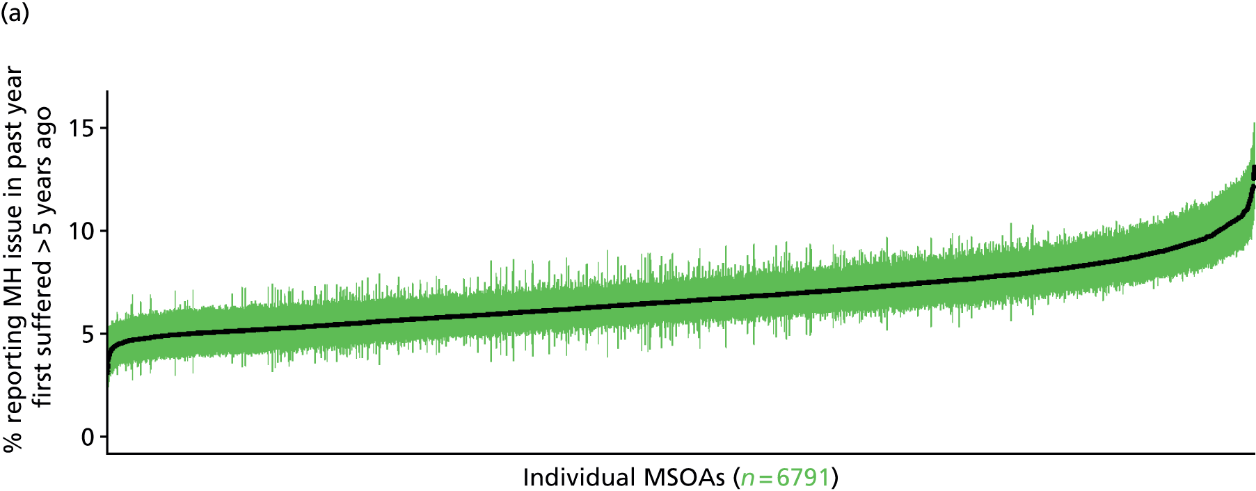

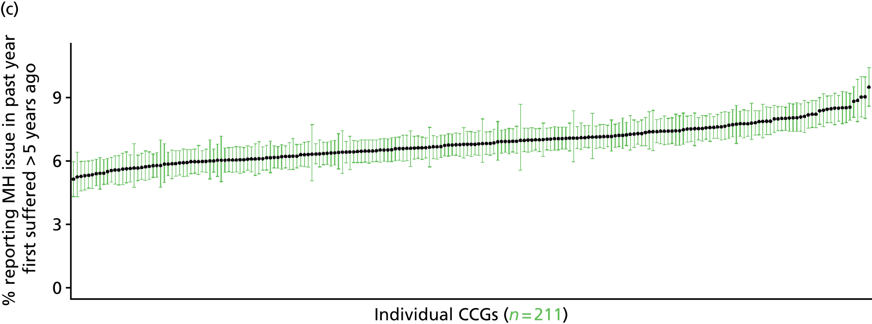
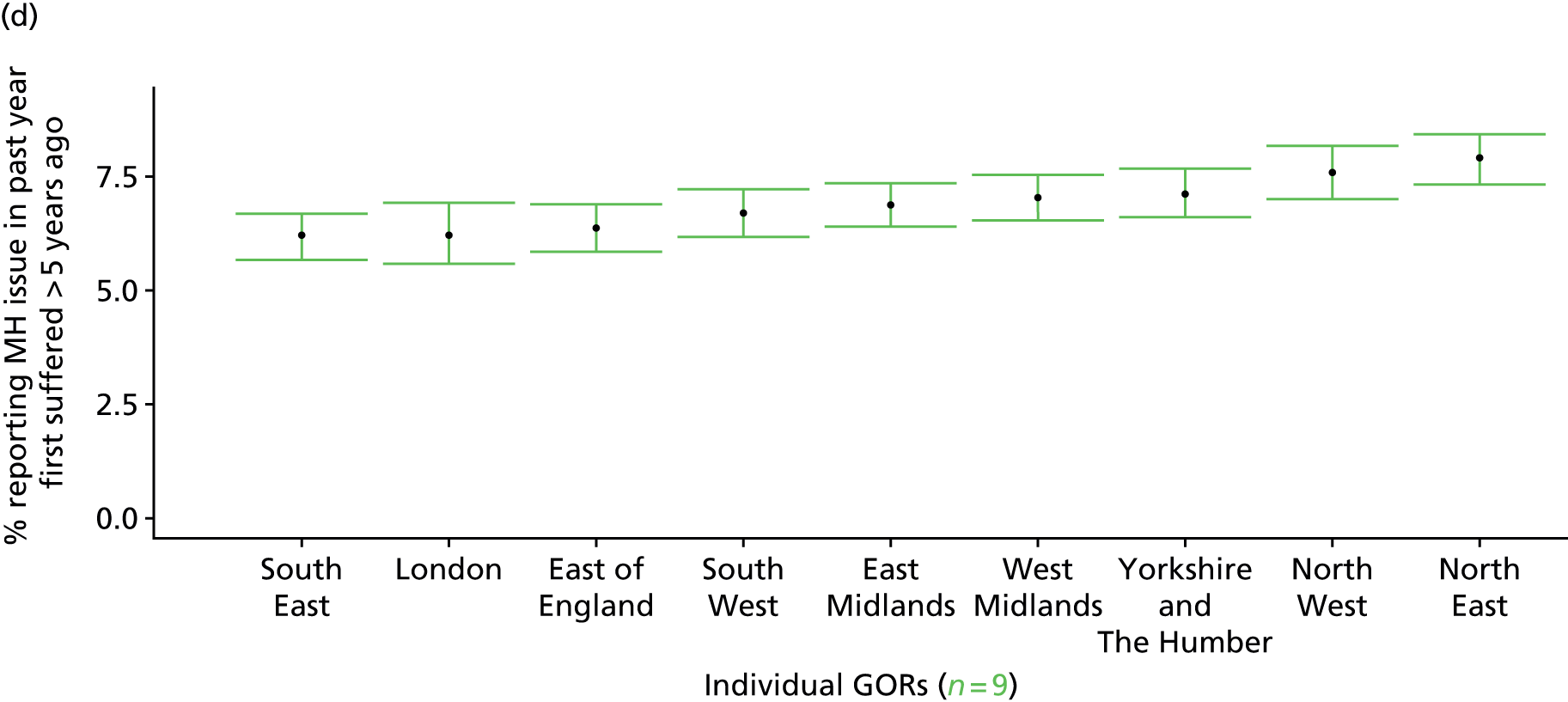
Self-reported long-standing mental health problem (Health Survey for England, 2006–11)
FIGURE 208.
Self-reported long-standing mental health problem: LSOA-level map. Contains Ordnance Survey data © Crown copyright and database right 2012.
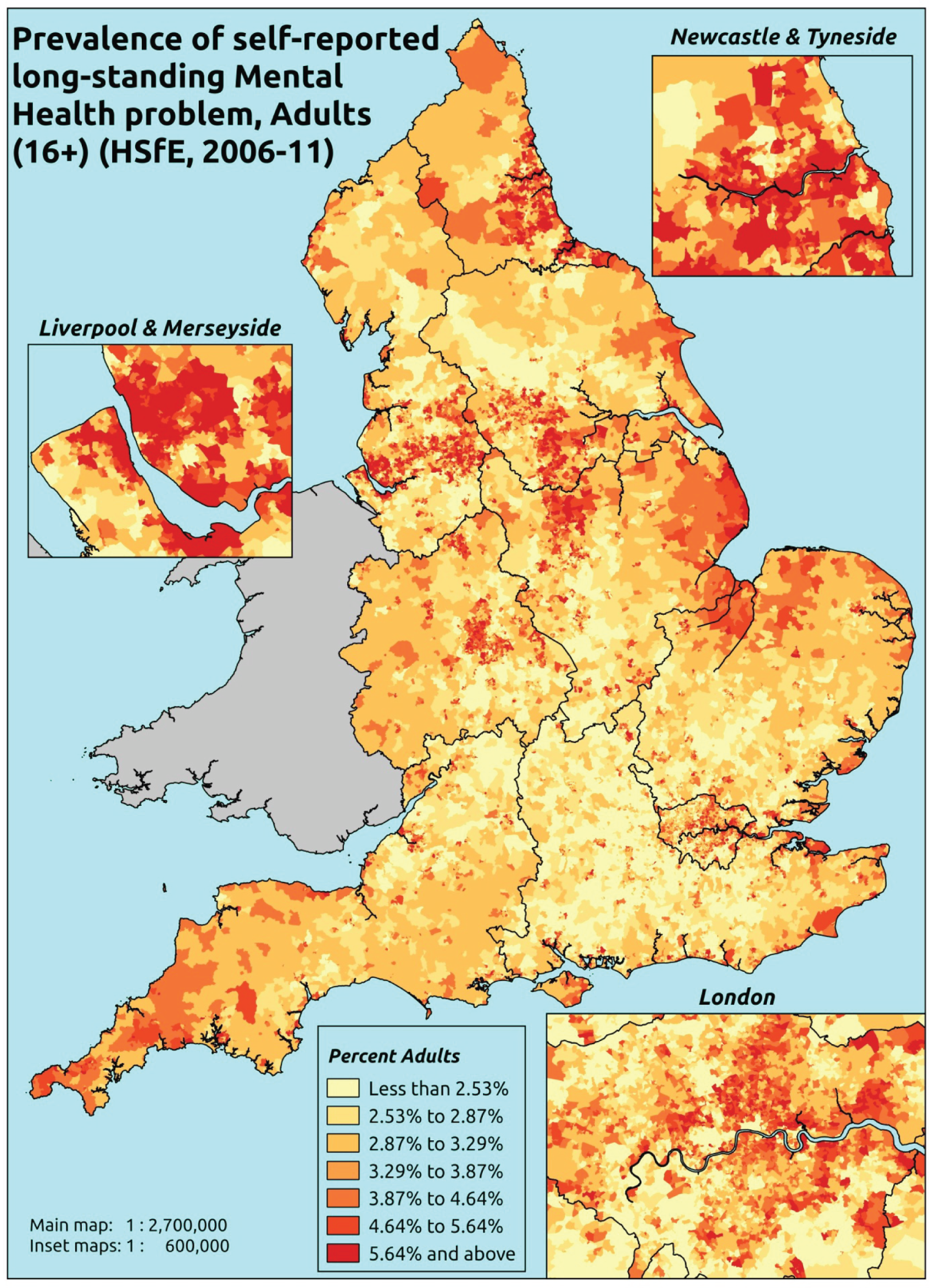
Response variable definition, provenance and prediction
Based on an open-ended question asked annually of all HSfE respondents: ‘Do you have any long-standing illness, disability or infirmity? By long-standing I mean anything that has troubled you over a period of time, or that is likely to affect you over a period of time?’ Responses are then categorised under a number of standard headings, including ‘04 Mental illness/anxiety/depression/nerves (nes)’.
Interestingly, and perhaps counterintuitively, there is surprisingly little overlap between those currently being prescribed medication for a mental health problem (BNF 4.1.x–4.6.x and 4.10.x–4.11.x487) and those self-reporting a long-standing mental health problem. Thus, as shown in Table 229, although 2.5% of all adult (≥ 16 years) respondents in the 2006–11 HSfE were self-reporting a mental health problem and being prescribed mental health medication, 1.4% of adults self-reported a mental health problem without being prescribed mental health medication (although we have no evidence on other treatments, such as IAPT or other psychological therapies), and fully 6.8% were being prescribed mental health medication while not admitting to a long-standing mental health problem. In other words, 73% of people being prescribed mental health medication did not see themselves as having a mental health problem.
| Self-reported long-standing mental health problem? | Respondents | Percentages | ||||
|---|---|---|---|---|---|---|
| Not currently prescribed mental health drugs | Currently prescribed mental health drugs | Total | Not currently prescribed mental health drugs | Currently prescribed mental health drugs | Total | |
| No | 36,373 | 2779 | 39,152 | 89.2% | 6.8% | 96.0% |
| Yes | 586 | 1030 | 1616 | 1.4% | 2.5% | 4.0% |
| Total | 36,959 | 3809 | 40,768 | 90.7% | 9.3% | 100.0% |
A very similar pattern is observed if one restricts the range of drugs to hypnotics and anxiolytics (BNF 4.1.1–4.1.3487) and antidepressants (BNF 4.3.1–4.3.4487), as shown in Table 230.
| Self-reported long-standing mental health problem? | Respondents | Percentages | ||||
|---|---|---|---|---|---|---|
| Not currently prescribed drugs for anxiety/depression | Currently prescribed drugs for anxiety/depression | Total | Not currently prescribed drugs for anxiety/depression | Currently prescribed drugs for anxiety/depression | Total | |
| No | 36,792 | 2360 | 39,152 | 90.2% | 5.8% | 96.0% |
| Yes | 686 | 930 | 1616 | 1.7% | 2.3% | 4.0% |
| Total | 37,478 | 3290 | 40,768 | 91.9% | 8.1% | 100.0% |
It is difficult to satisfactorily account for this dislocation between self-reported long-standing mental health problems and use of prescription drugs. Presumably some individuals on medication do not consider their mental health problems to be long-standing, but one must suspect that a majority of respondents on medication simply feel that their mental health problem is being sufficiently well contained that it has not ‘troubled’ them over a period of time, and is not likely to in the future. To that extent the presence of a self-reported mental health problem cannot be taken as a marker of health care. What we have here seems to be a marker of a recognised but unresolved mental health problem. Once again, this statistic is likely to be affected by sociodemographic and/or geographic variations in access to, or uptake of, prescribing – particularly if it is indeed the treatment people receive which means that respondents are able to ‘dismiss’ the fact that they may have a longstanding mental health problem.
The HSfE at this time includes multiple household respondents of all ages. The analytical data set is drawn from a subset of respondents aged ≥ 16 years for whom data are available across all model response and predictor variables, namely whether or not they responded to this EQ-5D question, along with information on age band, sex, ethnicity, general health status, LLTI, tenure and the IMD quintile of the LSOA of residence (n = 57,363). A single randomly selected adult is then drawn from each household, resulting in an analytical data set of 30,228 adults aged ≥ 16 years.
| Age band (years) | Females | Age band (years) | Males | ||||
|---|---|---|---|---|---|---|---|
| Does not have condition | Has condition | % | Does not have condition | Has condition | % | ||
| 16–24 | 727 | 38 | 5.0 | 16–24 | 444 | 12 | 2.6 |
| 25–34 | 2382 | 144 | 5.7 | 25–34 | 1638 | 69 | 4.0 |
| 35–49 | 4666 | 278 | 5.6 | 35–49 | 3461 | 184 | 5.0 |
| 50–64 | 3823 | 242 | 6.0 | 50–64 | 3653 | 177 | 4.6 |
| 65–74 | 2030 | 53 | 2.5 | 65–74 | 2123 | 43 | 2.0 |
| 75–84 | 1673 | 39 | 2.3 | 75–84 | 1293 | 22 | 1.7 |
| ≥ 85 | 649 | 15 | 2.3 | ≥ 85 | 344 | 6 | 1.7 |
| Females | 15,950 | 809 | 4.8 | Males | 12,956 | 513 | 3.8 |
| Total (males and females) | 28,906 | 1322 | 4.4 | ||||
Model parameters are applied to microsimulated LSOA-level census data to produce estimates of the number (and proportion) of people expected to report a long-standing mental health problem in each age–sex cohort (and overall) in each of the 32,844 English LSOAs. As discussed in the report, bootstrapping is used to derive 95% CIs for the estimates. These LSOA-level prevalence rate estimates (and 95% CIs) are aggregated into a number of higher geographies, namely MSOAs, LAs, CCGs and regions (GORs). Proportionate attribution is used to restructure the prevalence rate estimates to align with 2001 MSOAs, as well as GP practice populations as defined by the 2011 NHS ADS.
Table 232 summarises how expected prevalence rates vary by age, sex and local deprivation (as measured by the 2010 IMD). There are 6569 LSOAs (with 9,226,227 adults) classified as being in the least deprived quintile; 6568 LSOAs (9,525,344 adults) in the second least deprived quintile; 6568 LSOAs (9,658,444 adults) in the third least deprived quintile; 6,568 LSOAs (9,650,576 adults) in the fourth least deprived quintile; and 6568 LSOAs (9,535,167 adults) in the most deprived quintile. Note that, as a general rule, variations in prevalence rates reflect variations in the socioeconomic composition of populations in the different types of LSOA rather than variations in deprivation per se.
| Cohort | Least deprived quintile LSOAs | Second least deprived quintile LSOAs | Third least deprived quintile LSOAs | Fourth least deprived quintile LSOAs | Most deprived quintile LSOAs | All England |
|---|---|---|---|---|---|---|
| Female 16–24 | 1.2 (0.5 to 1.9) | 1.3 (0.7 to 2.1) | 1.7 (1.0 to 2.5) | 2.2 (1.4 to 3.0) | 2.6 (1.9 to 3.5) | 1.9 (1.2 to 2.7) |
| Female 25–34 | 2.9 (2.3 to 3.5) | 3.0 (2.4 to 3.5) | 3.6 (3.0 to 4.1) | 4.4 (3.8 to 4.9) | 5.1 (4.5 to 5.8) | 4.0 (3.5 to 4.4) |
| Female 35–49 | 3.4 (2.8 to 3.8) | 3.8 (3.2 to 4.3) | 5.0 (4.3 to 5.6) | 6.7 (5.8 to 7.4) | 8.2 (7.2 to 9.0) | 5.4 (4.8 to 5.8) |
| Female 50–64 | 4.2 (3.5 to 4.8) | 4.7 (4.0 to 5.3) | 6.0 (5.2 to 6.8) | 7.9 (6.9 to 9.0) | 9.3 (8.3 to 10.7) | 6.2 (5.6 to 6.9) |
| Female 65–74 | 2.6 (2.0 to 3.2) | 2.7 (2.1 to 3.5) | 3.3 (2.6 to 4.0) | 4.1 (3.1 to 5.0) | 4.2 (3.3 to 5.2) | 3.3 (2.6 to 4.0) |
| Female ≥ 75 | 3.0 (2.1 to 3.6) | 3.0 (2.2 to 3.8) | 3.5 (2.7 to 4.4) | 4.1 (3.1 to 5.0) | 3.8 (2.8 to 4.9) | 3.4 (2.7 to 4.2) |
| Females | 3.1 (2.5 to 3.7) | 3.4 (2.8 to 4.0) | 4.2 (3.5 to 4.9) | 5.3 (4.4 to 6.1) | 6.1 (5.2 to 7.0) | 4.4 (3.8 to 5.0) |
| Male 16–24 | 0.9 (0.5 to 1.4) | 1.0 (0.6 to 1.6) | 1.4 (0.9 to 2.0) | 1.9 (1.3 to 2.6) | 2.7 (2.0 to 3.5) | 1.7 (1.2 to 2.3) |
| Male 25–34 | 2.0 (1.6 to 2.4) | 2.1 (1.8 to 2.5) | 2.6 (2.3 to 3.1) | 3.4 (3.0 to 3.8) | 4.5 (4.0 to 5.2) | 3.1 (2.8 to 3.6) |
| Male 35–49 | 2.1 (1.7 to 2.5) | 2.6 (2.1 to 2.9) | 3.5 (3.1 to 4.0) | 5.1 (4.5 to 5.7) | 7.2 (6.4 to 8.1) | 4.1 (3.7 to 4.5) |
| Male 50–64 | 2.8 (2.3 to 3.2) | 3.3 (2.8 to 3.8) | 4.4 (3.8 to 5.3) | 6.4 (5.6 to 7.4) | 8.3 (7.5 to 9.6) | 4.9 (4.4 to 5.5) |
| Male 65–74 | 1.7 (1.3 to 2.2) | 1.9 (1.5 to 2.5) | 2.4 (1.9 to 3.1) | 3.1 (2.4 to 4.0) | 3.5 (2.8 to 4.5) | 2.4 (2.0 to 3.0) |
| Male ≥ 75 | 1.9 (1.4 to 2.4) | 1.9 (1.5 to 2.6) | 2.4 (1.8 to 3.1) | 2.9 (2.3 to 3.7) | 3.0 (2.3 to 4.0) | 2.4 (1.9 to 3.0) |
| Males | 2.1 (1.6 to 2.5) | 2.4 (1.9 to 2.8) | 3.1 (2.6 to 3.7) | 4.2 (3.6 to 4.9) | 5.5 (4.8 to 6.4) | 3.4 (3.0 to 4.0) |
| All | 2.6 (2.2 to 2.9) | 2.9 (2.5 to 3.3) | 3.6 (3.3 to 4.1) | 4.8 (4.3 to 5.2) | 5.8 (5.3 to 6.3) | 4.0 (3.7 to 4.2) |
| Factor (reference group) | Model coefficients | 95% CI | ||
|---|---|---|---|---|
| Estimate | SE | 2.5% CI | 97.50% | |
| (Intercept) | –6.79508 | 0.79181 | –8.34702 | –5.24314 |
| Age (16–24 years) | ||||
| 25–34 years | 1.65553 | 0.79558 | 0.09620 | 3.21487 |
| 35–49 years | 1.87656 | 0.78253 | 0.34280 | 3.41032 |
| 50–64 years | 1.77963 | 0.78466 | 0.24169 | 3.31757 |
| 65–74 years | 1.27734 | 0.80621 | –0.30284 | 2.85751 |
| 75–84 years | 1.31947 | 0.81630 | –0.28048 | 2.91942 |
| ≥ 85 years | –11.70700 | 183.49721 | –371.36154 | 347.94754 |
| Sex (females) | ||||
| Males | –0.71655 | 0.13897 | –0.98894 | –0.44416 |
| Ethnicity (white) | ||||
| Mixed | –0.17813 | 0.28754 | –0.74170 | 0.38545 |
| Black | –0.58186 | 0.17214 | –0.91924 | –0.24447 |
| Asian | –1.44568 | 0.30316 | –2.03987 | –0.85148 |
| Other | –0.62763 | 0.45913 | –1.52753 | 0.27228 |
| General health status (very good health) | ||||
| Good health | 0.94617 | 0.17035 | 0.61229 | 1.28005 |
| Fair health | 1.88629 | 0.18403 | 1.52559 | 2.24700 |
| Bad health | 2.59859 | 0.32908 | 1.95358 | 3.24359 |
| Very bad health | 3.13191 | 0.56661 | 2.02134 | 4.24247 |
| LLTI (no LTTI) | ||||
| LLTI | 3.55988 | 0.42736 | 2.72226 | 4.39749 |
| Tenure (owner–occupier) | ||||
| Social rent | 1.80924 | 0.77058 | 0.29890 | 3.31957 |
| Private rent or other tenure | 1.46351 | 0.77232 | –0.05024 | 2.97725 |
| LSOA deprivation quintile (least deprived quintile) | ||||
| Second quintile | –0.04968 | 0.11419 | –0.27349 | 0.17412 |
| Third quintile | 0.05808 | 0.10885 | –0.15527 | 0.27143 |
| Fourth quintile | 0.17668 | 0.10630 | –0.03166 | 0.38503 |
| Fifth quintile ( = most deprived quintile) | 0.08311 | 0.10900 | –0.13053 | 0.29675 |
| Interaction effects | ||||
| 25–34 years and LLTI | –0.40779 | 0.39564 | –1.18326 | 0.36767 |
| 35–49 years and LLTI | –1.16162 | 0.37346 | –1.89361 | –0.42963 |
| 50–64 years and LLTI | –1.45454 | 0.37954 | –2.19845 | –0.71064 |
| 65–74 years and LLTI | –1.89815 | 0.43336 | –2.74755 | –1.04876 |
| 75–84 years and LLTI | –2.56334 | 0.45679 | –3.45865 | –1.66802 |
| ≥ 85 years and LLTI | 10.938320 | 183.49599 | –348.71382 | 370.590460 |
| Male and social rent | 0.77654 | 0.13954 | 0.50305 | 1.05004 |
| Male and private rent or other tenure | 0.24249 | 0.18815 | –0.12628 | 0.61125 |
| 25–34 years and social rent | –1.34892 | 0.79313 | –2.90345 | 0.20561 |
| 35–49 years and social rent | –1.09327 | 0.77826 | –2.61866 | 0.43212 |
| 50–64 years and social rent | –1.57804 | 0.77909 | –3.10506 | –0.05102 |
| 65–74 years and social rent | –2.30459 | 0.81071 | –3.89358 | –0.71560 |
| 75–84 years and social rent | –1.76754 | 0.81942 | –3.37361 | –0.16147 |
| ≥ 85 years and social rent | –2.60182 | 0.9347 | –4.43384 | –0.76981 |
| 25–34 years and private rent or other tenure | –1.16539 | 0.79734 | –2.72817 | 0.39739 |
| 35–49 years and private rent or other tenure | –1.11734 | 0.78904 | –2.66386 | 0.42918 |
| 50–64 years and private rent or other tenure | –0.92503 | 0.79384 | –2.48096 | 0.63091 |
| 65–74 years and private rent or other tenure | –1.07728 | 0.87441 | –2.79113 | 0.63656 |
| 75–84 years and private rent or other tenure | –1.01182 | 0.94135 | –2.85686 | 0.83321 |
| ≥ 85 years and private rent or other tenure | –0.75172 | 1.10436 | –2.91626 | 1.41281 |
| Good health and LLTI | –0.61271 | 0.27205 | –1.14593 | –0.07948 |
| Fair health and LLTI | –0.87063 | 0.27319 | –1.40609 | –0.33517 |
| Bad health and LLTI | –1.33602 | 0.38832 | –2.09713 | –0.57491 |
| Very bad health and LLTI | –1.67931 | 0.60965 | –2.87422 | –0.48439 |
| Male and LLTI | 0.27043 | 0.14713 | –0.01795 | 0.55880 |
FIGURE 209.
Parameter plots: self-reported long-standing mental health problem.
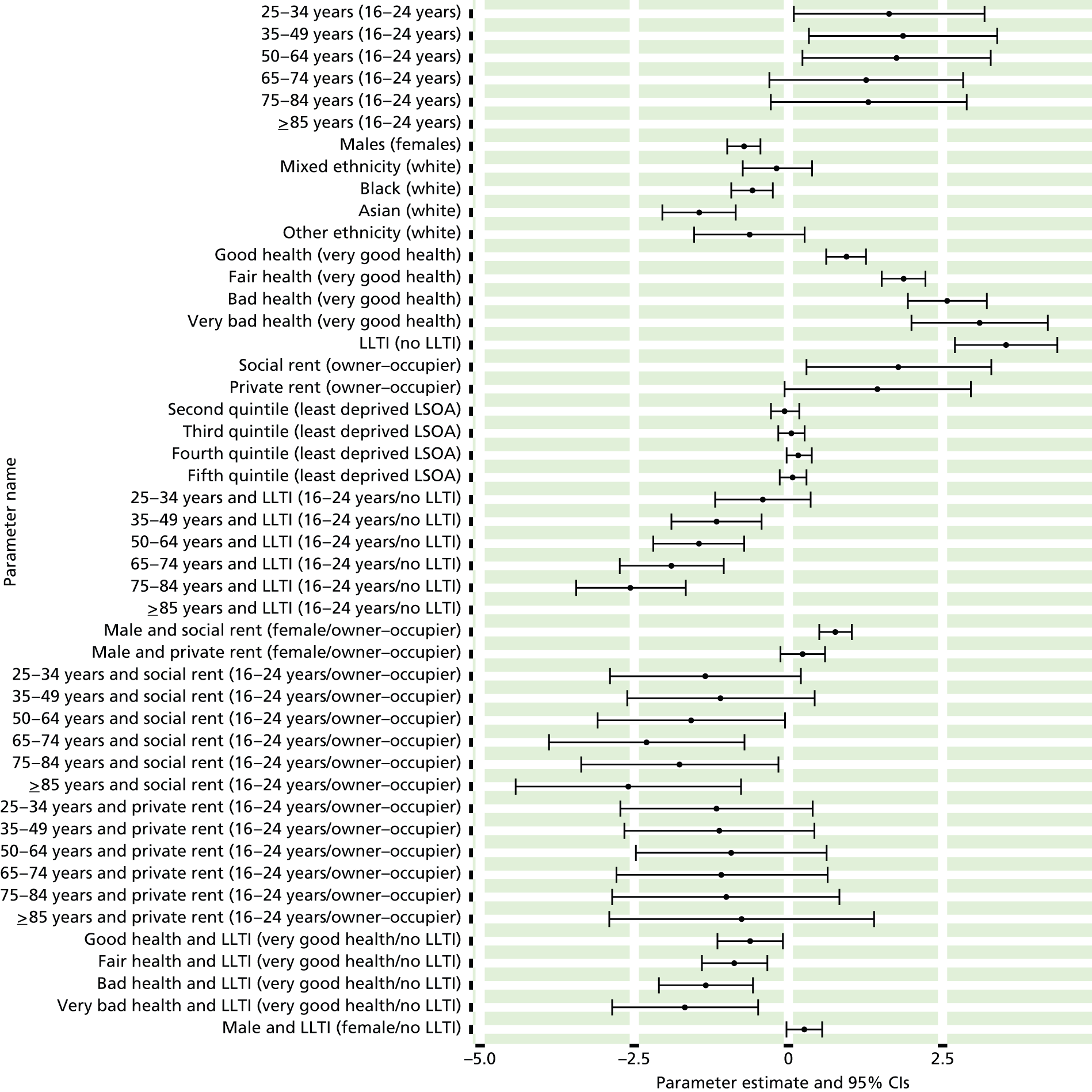
FIGURE 210.
Self-reported long-standing mental health problem: individual estimates and their 95% CIs. (a) MSOAs; (b) LAs; (c) CCGs; and (d) regions (GORs). LS, long-standing; MH, mental health.


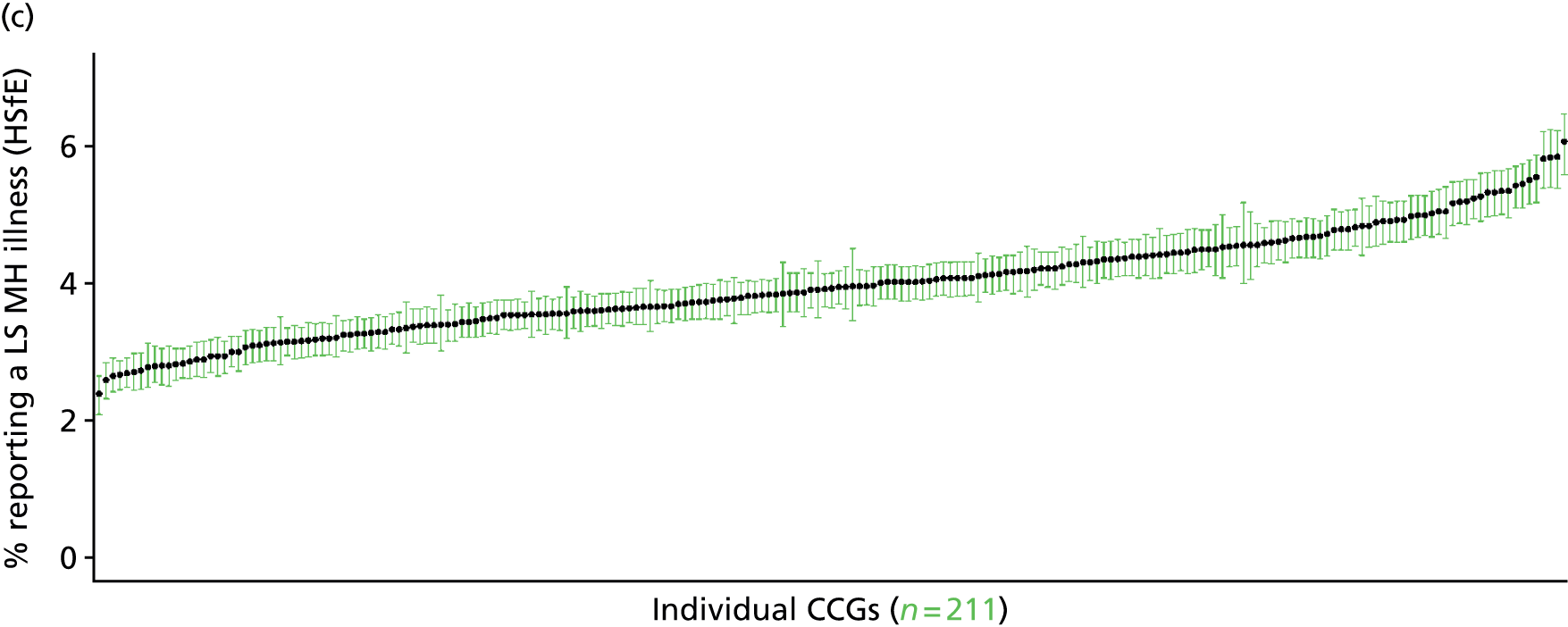
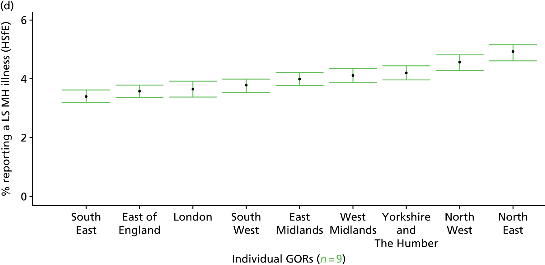
Glossary
- Access
- The processes by which people gain entry to the health-care system (or from lower to higher levels of the health-care system), which may be measured through service availability, service utilisation, service quality and service outcomes.
- Adjudication
- The process by which claims to candidacy (or expressed need) are judged and acted on by health professionals. Again, systematic differences in adjudication at the population level are of interest in this quantitative study. For example, are there differences in the primary or specialist management of disease according to age, sex, socioeconomic status or ethnicity?
- Candidacy
- The way(s) in which people recognise their eligibility for medical attention, leading them to express their needs to health professionals. A key issue is whether or not and how demand-side factors influence this process.
- Deep end
- A term often applied to socioeconomically deprived areas with populations suffering complex and interacting physical and mental health problems, financial difficulties, social and emotional problems, substance abuse, chaotic lifestyles, etc. The expression aims to highlight the difficulties local general practitioners face in such areas.
- Demand-side factors
- Factors that influence a person’s decision to seek health care in the first place, or to accept offers of care. In addition to clinical need, these may include knowledge, information, psychological fears such as fear or stigma and practical issues such as difficulties in taking time off work. Here, we are interested in systematic differences in the ways in which people express candidacy at a population level. For example, are people of lower socioeconomic status less or more likely to seek health care for the same symptoms?
- Extra-welfarism
- An economic theory that departs from traditional welfare economics by prioritising outcomes over utility, allowing gains in health to outweigh losses and promoting social over individual values.
- Health-care equity
- Equal availability or equal utilisation or health care for those in equal clinical need of health care.
- Health equity
- Equality in terms of health outcomes (i.e. no inequalities in health status).
- Horizontal equity
- The equal treatment of equals (i.e. those who have equal levels of clinical need have equal access to health care).
- Illegitimate variation
- Variations in access which reflect unmet need or unjustified supply.
- Inverse care law
- An observation first made by Julian Tudor Hart in 1971, whereby the availability of good medical care varies inversely with the need for it in the population served. Tudor Hart was particularly concerned with inverse care in the distribution of general practitioners. However, the term is now applied beyond primary care and tends to be associated with the needs of socioeconomically deprived populations.
- Legitimate variation
- Variations in utilisation which reflect variations in underlying need.
- Residualism
- Access to welfare is targeted at those who fall below a certain (e.g. income) threshold (see also Selectivism). This approach is associated with means testing and social stigmatisation, although targeted approaches to NHS provision have avoided this association because the NHS is still classed as a universal service.
- Rule of rescue
- Health care is provided in response to immediate clinical need.
- Selectivism
- Access to welfare excludes those who are not considered sufficiently needy (see also Residualism); that is, access is targeted.
- Supply-side factors
- System/organisational factors that affect people’s ability to access care. Includes lack of capacity (e.g. to provide specialist services or to ensure reasonable waiting times); variations in quality (e.g. single-handed practice issues, specialist vs. generalist consultants); and differences in resource allocation and features of service configuration (e.g. access to regional centres).
- Universalism
- The unconditional and (other than responding to need) unfixed provision of social welfare for all, financed by government on a non-discriminatory basis. It is the opposite of selective or residual welfare.
- Vertical equity
- The unequal treatment of equals (i.e. those who have equal levels of clinical need) in order to achieve a greater equality in health outcomes (such as life expectancy).
- Weighted capitation
- The approach by which per-capita needs for NHS funding are determined. In England, this has been dominated by an econometric approach (where need for services over and above that determined by age and sex and unavoidable differences in cost is established through the regression modelling of use of services, attempting to control for supply).
List of abbreviations
- A&E
- accident and emergency
- ACE
- angiotensin-converting-enzyme
- ADS
- Attribution Data Set
- APHO
- Association of Public Health Observatories
- APMS
- Adult Psychiatric Morbidity Survey
- ARB
- angiotensin receptor blocker
- AREA
- Allocation of Resources to English Areas
- BNF
- British National Formulary
- CABG
- coronary artery bypass graft
- CCG
- Clinical Commissioning Group
- CHD
- coronary heart disease
- CI
- confidence interval
- CIS-R
- Clinical Interview Schedule – Revised
- CKD
- chronic kidney disease
- CMHD
- common mental health disorder
- COPD
- chronic obstructive pulmonary disease
- CRD
- Centre for Reviews and Dissemination
- CRHT
- crisis resolution and home treatment
- CVD
- cardiovascular disease
- GHQ12
- 12-item General Health Questionnaire
- GHS
- General Household Survey
- GOR
- Government Office Region
- GP
- general practitioner
- HSCIC
- Health and Social Care Information Centre
- HSfE
- Health Survey for England
- IAPT
- Improving Access to Psychological Therapies
- IMD
- Index of Multiple Deprivation
- LA
- local authority
- LLTI
- limiting long-term illness
- LSI
- long-standing illness
- LSOA
- lower-layer super output area
- MI
- myocardial infarction
- MSOA
- middle-layer super output area
- NEPHO
- North East Public Health Observatory
- NIC
- net ingredient cost
- NICE
- National Institute for Health and Care Excellence
- ONS
- Office for National Statistics
- PBC
- Programme Budget Category
- PCI
- percutaneous coronary intervention
- PCT
- primary care trust
- PHE
- Public Health England
- PSU
- primary sampling unit
- QALY
- quality-adjusted life-year
- QOF
- Quality and Outcomes Framework
- RCGP
- Royal College of General Practitioners
- SHA
- Strategic Health Authority
- SMR
- standardised mortality rate
- TIA
- transient ischaemic attack
- UKHLS
- UK Household Longitudinal Study