Notes
Article history
The research reported in this issue of the journal was funded by the HTA programme as project number 11/46/03. The contractual start date was in October 2012. The draft report began editorial review in September 2016 and was accepted for publication in January 2017. The authors have been wholly responsible for all data collection, analysis and interpretation, and for writing up their work. The HTA editors and publisher have tried to ensure the accuracy of the authors’ report and would like to thank the reviewers for their constructive comments on the draft document. However, they do not accept liability for damages or losses arising from material published in this report.
Declared competing interests of authors
none
Permissions
Copyright statement
© Queen’s Printer and Controller of HMSO 2017. This work was produced by Birrell et al. under the terms of a commissioning contract issued by the Secretary of State for Health. This issue may be freely reproduced for the purposes of private research and study and extracts (or indeed, the full report) may be included in professional journals provided that suitable acknowledgement is made and the reproduction is not associated with any form of advertising. Applications for commercial reproduction should be addressed to: NIHR Journals Library, National Institute for Health Research, Evaluation, Trials and Studies Coordinating Centre, Alpha House, University of Southampton Science Park, Southampton SO16 7NS, UK.
Chapter 1 Background
Each year, the UK government publishes a document entitled the ‘National Risk Register of Civil Emergencies’. The latest edition of the register lists the outbreak of a pandemic influenza virus to be the highest priority non-terrorism risk faced by the UK population. 1 This highlights the importance of the country being in a high state of preparedness for such an outbreak. A key component of any protocol governing the public health response to an outbreak is a plan to monitor and predict the progress of a pandemic in real time.
During the 2009 outbreak of pandemic A/H1N1 influenza, much attention was devoted to the problem of capturing the epidemic dynamics through real-time modelling. The aim of such modelling was to provide up-to-the-moment assessments of the state of the epidemic, as well as to make predictions about its future course, all based on continually updating streams of information. The models used are mathematical constructs, that is, systems of equations designed to approximate epidemic dynamics, describing the changes over time in the number of people within a population who are susceptible to infection, the number currently infected and the number who are presently immune. These equations are governed by a few key (hitherto unknown) quantities known as parameters, which usually represent a physical characteristic of the epidemic (e.g. the average duration of infection or the relative rates of contact between members of relevant population groups). To enable assessment of the current state of the epidemic and its future evolution, values for these parameters need to be identified that are consistent with epidemic data. In addition, the uncertainty in the parameter values needs to be properly reflected in such assessments. To make formal, statistical estimations of model parameters, models can often be simplified to ensure that estimates can be derived from the available data, computational resources and expertise. More generally, as seen in research focused on the evaluation of in-pandemic mitigation strategies,2,3 parameter estimates have been obtained on a more ad hoc basis by using the models and assumed ranges of parameter values to simulate epidemic scenarios. A selection of these parameter values is then retained based on some informal comparison between the corresponding simulated epidemics and the observed data. This type of approach is common to the literature on real-time modelling prior to 2009, in which the proposed methodologies are heavily reliant on an idealised set of circumstances and/or on ad hoc estimation methods. 4
Bayesian statistical epidemic models provide a natural, rigorous framework for the incorporation of relevant contemporaneous surveillance data into the modelling process, alongside collateral information that may be available from other sources. Such models have been used in the context of real-time monitoring for other infectious diseases. For severe acute respiratory syndrome, models have been proposed and applied for real-time estimation where the focus is on the reproductive number,5–7 a key epidemic characteristic often denoted R0. A more complex Bayesian approach is utilised in an application to data stemming from the avian influenza epidemic in the UK poultry industry. 8 Here, the availability of individual-level data and the use of computationally intensive Bayesian techniques make it possible to carry out inference on the transmission dynamics, rather than merely the reproductive number. A similar model has been formulated within the Bayesian statistical paradigm to provide real-time estimates of the time-evolving effective reproductive number R0(t) for a generic emerging disease,9 an approach that has since been applied to an A/H7N9 outbreak in China10 and subsequently extended to a more complex version of the model. 11
However, the modelling approaches above have typically used a single data stream providing direct data on the number of new cases of an infectious disease over time. This is also the case in the context of the 2009 outbreak in Singapore,12 where a real-time reporting system for influenza-like illness (ILI) in sentinel general practices (GPs) was established, and the resulting data were used to predict the epidemic in real time. In practice, as illustrated by the 2009 outbreak in the UK, direct data are seldom available and it is more likely that multiple sources of data exist, each indirectly informing the epidemic development and each subject to possible sources of bias. This calls for more involved complex epidemic modelling that can synthesise the information held within a range of data sources to compensate for the lack of direct observation of the infection process. As a result of this, real-time modelling in the UK in the face of the 2009 A/H1N1pdm outbreak proved to be more demanding and more intricate than had been anticipated. 13
In response to the 2009 pandemic in England, two approaches to real-time modelling were developed. 14,15 In the first,14 the authors present a framework for the real-time assessment of the effectiveness and cost-effectiveness of vaccination strategies, considering the whole of England. Embedded inside a cost-effectiveness model is an age and risk group structured deterministic mass-action susceptible, exposed, infectious, recovered (SEIR) transmission model, parameterised in terms of an age-specific force of infection, that is, the rate at which susceptible individuals acquire infection. Model parameters are estimated by a hybrid of ad hoc approaches using the estimated weekly numbers of symptomatic cases routinely produced by the Health Protection Agency (HPA) [from 2011, Public Health England (PHE)] as data during the outbreak. 16 Uncertainty in key parameters (e.g. R0) is generated by sampling values of each parameter from a range or distribution to form a ‘scenario’ from each combination of parameter values. Results from each scenario are compared with the scaled estimates, and only the best-fitting 1% of the 60,000 realisations are retained to simulate future incidence and evaluate, with epidemiological uncertainty, the impact of different vaccination strategies on severe outcomes.
In the second approach,15 data were more directly utilised within a Bayesian statistical framework. The basic modelling features resemble those used to measure the effects of school closure as a strategy for epidemic mitigation in Hong Kong. 17 The primary difference is in the data used. Instead of using counts of case confirmations alone, an array of different data sets were combined: age- and region-stratified data on GP consultations for ILI;18 virological positivity data from individuals reporting symptoms of ILI available through the Royal College of General Practitioners (RCGP) surveillance network and the Regional Microbiology Network (RMN) of the HPA; virological case confirmations from the early part of the epidemic; and data on the seropositivity of sera samples taken before and during the 2009 pandemic and held by the Weekly Returns Service of the RCGP. The modelling details of this second approach are detailed in Modelling methodology: single region model and Appendix 1 for more details. 19 This work, however, considered only the London region.
After the 2009 experience, two main issues were left unresolved. The first is the development of a spatial characterisation of the epidemic. This would need to be carried out at a geographical level fine enough to ensure homogeneous epidemic activity within each geographical unit, yet coarse enough to guarantee enough available data to ensure that each unit has a sufficiently informative sample size. The second issue is the need to accommodate the greater wealth of epidemic surveillance data supposedly available in future pandemics. 20
Both developments pose a challenge to existing modelling approaches. With regard to the Bayesian approach,15 the challenge is to extend the model structure and increase the number of pandemic data sets to be assimilated into an already complex model in a sufficiently timely fashion for analysis to be feasible in real time. This requires the development of more computationally efficient methods for Bayesian inference.
Computational methods
The Bayesian approach is based on a computational technique known as Markov chain Monte Carlo (MCMC). 21 MCMC can be computationally burdensome when estimation and prediction of an evolving epidemic are needed in real time. Every time new data become available, MCMC reanalyses the data in their entirety, requiring possibly millions of evaluations of the model. This is computationally costly and will, consequently, limit the speed at which results can be obtained.
There are existing methods to approximate the estimation procedure, either by replacing the model with a more-readily evaluated proxy22 or by approximating the Bayesian approach. 23 However, sequential Monte Carlo (SMC) methods are a more appropriate alternative to MCMC. 24–26 The use of such methods to analyse epidemic data is relatively common,11,27 yet analyses with a real-time focus are rare,12 and those using a synthesis of numerous types of data do not exist.
A further complication, which is not considered in the existing literature, is the need to accommodate the impact that public health interventions might have on the surveillance data underpinning the real-time analysis. As infection becomes more widespread, health-care facilities become harder to access, with those in need of health care channelled elsewhere. Any effective real-time computational approach has to cope with the sudden shocks, unforeseen in some cases, that interventions might generate on the time course of the surveillance data.
Outline
The work reported here will expand on an existing framework for statistical epidemic modelling,15 increasing its complexity to allow for spatial heterogeneity in transmission. Two competing spatial modelling approaches are examined (see Chapter 3, Modelling methodology: multi-region models and Chapter 4, Spatial modelling) to investigate how epidemic activity in different regions can be most efficiently and accurately estimated. This increased complexity and the extra dimension added to each of the epidemic data sets add to the computational burden. A general algorithm for Bayesian statistical inference in such a scenario is developed and tested on a suite of synthetic pandemic data, incorporating the presence of ‘shocks’ in surveillance data arising from public health interventions (see Chapter 3, Monte Carlo methods and Chapter 4, Comparison of the real-time performance of the Monte Carlo methods). The report concludes with a discussion (see Chapter 5) and recommendations for future research (see Chapter 6).
Chapter 2 Study objectives
The central objective of this study is to advance the state of the art of real-time modelling of influenza epidemics and to provide a useful tool that can be used to monitor and predict the development of an ongoing pandemic outbreak. This advancement involves:
-
accounting for spatial heterogeneity in transmission – this may be done through the modelling of separate, non-interacting but parametrically linked epidemics in spatially disjoint regions of a country, or through further stratification of the population according to location
-
building capacity in terms of the different types and increasing the number of data that can be used for real-time modelling
-
improving the efficiency with which real-time statistical inference can be made
-
developing a real-time inferential system that is robust to likely pandemic mitigation or treatment interventions.
A suite of software has been produced to achieve the above objectives and provide support to national public health bodies in the event of a pandemic. This software has been tailored to the specific requirements of PHE, the responsible public health body in England.
Initially, there was also a component of this research promising support to the HPA (now PHE) in the event of a pandemic in their real-time production of estimates and projections of the health-care burden attributable to the pandemic. Such an outbreak did not occur over the duration of the study, and so this component of the project has been disregarded in the report.
Chapter 3 Methods
We shall begin by describing the modelling approaches used in this work (see Modelling methodology: single region model and Modelling methodology: multi-region models). In Data we will examine the data types that PHE currently envisage being available at some stage during a pandemic and discuss how the structure of the available data from 2009 helped to determine the precise parameterisation of the real-time model. Together, the modelling approaches and data types will inform the spatial modelling study.
Bayesian inference provides an introduction to Bayesian inference and Monte Carlo methods discusses the MCMC and SMC methods. Monte Carlo methods, in particular, contains a significant amount of technical detail, including the tuning of a number of algorithmic components necessary to achieve timely inference, and may be omitted by the reader not interested in such detail.
Modelling methodology: single-region model
The starting point for the investigation in this study is the model and analysis of Birrell et al. 15 Here, information from multiple sources is integrated into a composite model, including:
-
an age-structured dynamic transmission component
-
a disease component
-
a component describing the mechanism of symptom reporting to health-care facilities.
A schematic model representation is given in Figure 1. Transmission in the SEIR model is governed by a time- and age-varying force of infection that is dependent on the population structure, the transmissibility of the virus, the mixing patterns between population strata and the expected time spent in the E (exposed) and I (infectious) states. In the disease model layer, a proportion, ϕ, of the newly exposed individuals develop febrile symptoms. In the reporting model layer, further proportions of these symptomatic individuals consult their GP and/or have their symptoms officially confirmed through a virologically positive swab result.
FIGURE 1.
A schematic diagram of the model. Adapted from Birrell et al. 15 © 2011 National Academy of Sciences.
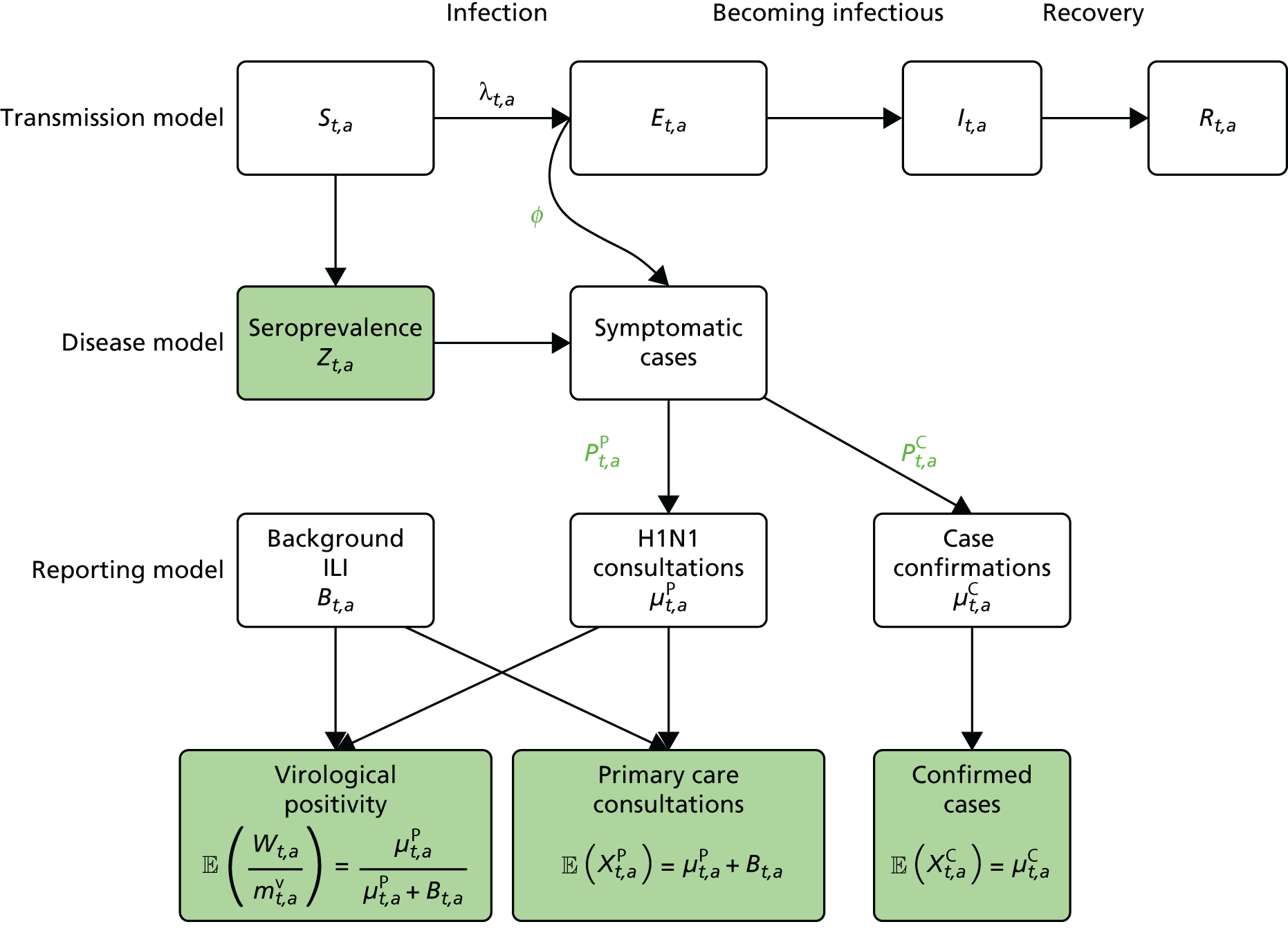
Ideally, direct data on the number of new infections would be available, and in studies of modelling methodology these types of data are often assumed. 11 However, more realistically, surveillance data sets are noisy and record events (such as GP consultations; see section entitled Pandemic data) that occur some time later than the infection. Specifically for influenza, disease reporting is frequently through syndromic surveillance, whereby non-disease specific symptoms are reported. Instead of reporting influenza infections, the reporting is of patients suffering with ILI. Therefore, data from such sources include contamination from patients carrying infections other than the pathogen of interest. This adds greater complexity to the task of disentangling the underlying disease incidence from the available information, particularly as this contamination is likely to vary substantially during the pandemic. To identify the disease incidence, these noisy consultation data are combined with information on virological positivity from complimentary surveillance systems (see Figure 1 and Data). When multiple time series data sets are available, data on events occurring as close as possible to the time of infection should be preferred, as they will be more informative. Alternatively, data arising as a result of severe symptoms are also valuable; severity is a property of the virus, and so the proportion of cases that appear in data will become more stable over time.
The equations governing the epidemic dynamics are included in Appendix 1.
Modelling methodology: multi-region models
The transmission model shown in Figure 1 and Appendix 1 is extended to accommodate spatial heterogeneity in the 2009 A/H1N1 pandemic data in two ways: (1) by using a parallel-region (PR) approach and (2) by using a meta-region (MR) approach. 28 These approaches will be introduced in the two following subsections, respectively.
The parallel-region model
In the PR modelling approach, the spatially heterogeneous epidemic is assumed to be composed of a number of smaller epidemics occurring in parallel within each spatial unit, with no direct interaction (specifically, no transmission) between regions. The rationale here is that the purpose of the real-time model is to monitor the pandemic once infection is widespread. By such a time, it is reasonable to assume that long-range inter-region transmission will be negligible in comparison with that occurring within each region.
The parallel epidemics are still jointly modelled; however, there is a sharing of information through a number of model parameters that either have a common value or a common temporal trend in each region. These parameters are typically those representing biological characteristics of the virus (mean infectious period, proportion symptomatic, etc.). Additionally, the mixing patterns are assumed to exhibit no regional variation. Appendix 1 presents a system of equations governing single-region dynamics. This system is driven by two key quantities: the reproductive number, R0, and the initial state of the system, defined by a parameter giving the initial number of infective individuals, I0. These are region specific parameters (R0,r, and I0,r, r = 1, . . . ,R) as they are functions of both the regional population and the virus. Together, these parameters account for the different timing of the pandemic activity in each region.
The system of dynamic equations given in Equation 18, Appendix 1 applies within each spatial unit, and so needs little modification.
The meta-region model
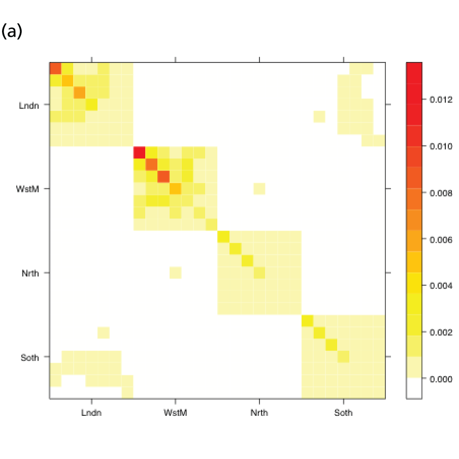
In the MR modelling approach, regions are assumed connected such that transmission is possible between individuals resident in different regions. Here, we look at the country as a whole and treat it as a metapopulation of R sub-regions. Therefore, we can generalise the notation in the system of equations (see Equation 18) in Appendix 1 so that the index a now takes values over the range 1, . . . ,RA. It is therefore necessary to define (RA × RA) contact matrices, Π(tk), k = 1, . . . ,K, that describe the rates at which individuals of the various (region- and age-defined) strata come into contact. In the single-region and PR models, this matrix describes the rates at which individuals of the various age groups interact, and was informed by UK data collected as part of the Improving Public Health Policy in Europe through the Modelling and Economic Evaluation of Interventions for the Control of Infectious Diseases (POLYMOD) study (see Equation 20 and relevant text). 29 In this expanded matrix, the entries that correspond to within-region contacts resemble the POLYMOD-based matrices. However, entries corresponding to inter-region interactions are typically of a lower order of magnitude, as people interact less frequently with others living in a different geographic region. These rates of contact are derived from census data on daily commuter movements between regions. The details of how, at the kth time point, tk, the POLYMOD matrices and the commuter data combine to produce contact matrices Π(tk) are given in Appendix 1. Figure 2 shows a heat map of the elements of Π(t1) as contact intensities on the absolute and log-scales. The strata are organised within regions, giving the matrix the appearance of an array of submatrix blocks within which the POLYMOD patterns of contact are repeated. The blocks on the diagonal give rates of within-region contact and, therefore, show much higher contact rates.
FIGURE 2.
Heat maps for the contact matrices used in the MR model (with regional density dependence) based on (a) contact rates; and (b) log-contact rates. The matrices show a strong, block-diagonal structure, with red areas indicating higher rates of contact. The blocks are ordered such that contacts involving residents of London are in the top row and in the first column, with the ordering of London, West Midlands, the North and, in the final row and column, the South. Within blocks, age is increasing from top to bottom and from left to right. Red squares indicate interactions of high frequency, white squares interactions of zero frequency. Adapted from Birrell et al. 28 © 2016, Macmillan Publishers Limited. This work is licensed under a Creative Commons Attribution 4.0 International License. The images or other third party material in this article are included in the article’s Creative Commons license, unless indicated otherwise in the credit line; if the material is not included under the Creative Commons license, users will need to obtain permission from the license holder to reproduce the material. To view a copy of this license, visit http://creativecommons.org/licenses/by/4.0/.

The MR model has only one system of dynamic equations of the type in shown in Equation 18 of Appendix 1, removing the flexibility of having region-specific values for R0 and the initial seeding of infectives, I0. However, there are a number of modelling considerations to be made when using the MR model, considerations that are not relevant to the PR modelling approach.
Density dependence
In a single-region model, the POLYMOD-based contact matrices give the relative frequency of contact between pairs of individuals of the different age groups. When these matrices are inserted into the block diagonal of the MR contact matrix (see Figure 2), an assumption of frequency-dependent contact is made. This implies that individuals are equally likely to have contact with any other individual in the region irrespective of the region in which they live. Therefore, individuals who live in regions with a higher population will make proportionately more contacts. This may not seem to be a reasonable assumption, as the total population of a region does not necessarily indicate a high population density. The alternative considered here is density-dependent contacts. In this case, the likelihood of a contact is scaled down by the population size, either of the regional population or of the strata (region and age) population. Both types of density dependence are considered.
Initial seeding of infectives
At the beginning of an epidemic, the transmission process is kick-started by a number of initial infectives. The POLYMOD-based contact matrices used for a single-region model (and in the PR model) will lead to rapid convergence towards a stable pattern of infection. In other words, for most reasonable choices of initial seeding, it takes only a short time for this seeding to be ‘forgotten’ by the transmission dynamics.
This is not the case in the MR model, with its block-structured matrix. Infection spreads very slowly between the regions, and so the initial seeding is not quickly forgotten. Epidemics seeded with infectives in different regions can lead to very different outcomes. Therefore, although the choice of the seeding in the PR model is not important, it is a significant modelling choice for the MR approach and a number of different seedings are considered: the single-region equilibrium distribution (i.e. the stable pattern of infection observed in the PR model) derived from the next generation matrix; the initial empirical age- and region-specific distribution of the initial confirmed cases; and a hybrid approach using a within-region equilibrium distribution scaled by the empirical distribution of the initial confirmed cases over regions.
Commuting at random
Each model makes the assumption of homogeneous mixing within each stratum. This means that all individuals within a population stratum are as likely to acquire or spread infection as any other individual of the same infection status. In the MR model, where infection is transmitted between regions through the routine movements of commuters, this assumption of homogeneity implies that on any day each individual is equally likely to commute. This is an unrealistic representation, however, as only a subset of people are likely to commute on a regular basis, and a (larger) subset are likely to stay within their home region. To account for this, adult age groups in each region are further subdivided into commuters and non-commuters, so that the commuters are a fixed group of people who move each day. This results in the effects of commuting on transmission being more transient, as there is a smaller, more rapidly exhaustible supply of susceptible individuals available to transfer infection from one region to another.
The downside to this further level of stratification is that it places an increased computational burden on the model, greatly slowing down the estimation process.
Data
During the 2009 pandemic, the HPA provided A/H1N1pdm incidence estimates for each of the then ten Strategic Health Authorities (SHAs) across England. Two of the SHAs, Greater London and the West Midlands, were believed to have experienced a significant, pre-summer wave of infection. Ideally, we would adopt the same geographical partition; however, the volume of data available from each of the SHAs is insufficient to do so. A reasonable compromise solution is to divide the country into four spatial units: London, the West Midlands (the two regions that had significant first waves of infection), the North and the South. The North and South regions each comprise four SHAs; in the North these are North East, North West, Yorkshire and Humberside, and East Midlands, and in the South they are East of England, South Central, South East Coast and South West.
The age categorisation favoured by the HPA, now PHE, is to break up the population into the age groups < 1 year, 1–4 years, 5–14 years, 15–24 years, 25–44 years, 45–64 years and ≥ 65 years. For the rest of this section, a will denote a general population stratum, whether defined by age alone or by both region and age.
The section, Pandemic data below, itemises the pandemic data streams that the real-time modelling framework is set up to work with, detailing, when applicable, how these data were used in modelling the 2009 pandemic and discussing how the various surveillance schemes have evolved over the intervening period. Distributional assumptions introduces some technical statistical details, showing how these data streams link into the SEIR transmission model, covering the distributional assumptions that are required to allow formal statistical inference to be made.
Pandemic data
General practice consultation data
Public Health England carry out syndromic surveillance to monitor influenza activity in the population by routinely collecting data on individuals presenting with an ILI at GPs. In 2009, such data were provided from two sources. The first source was the Weekly Returns Service of the RCGP, a sentinel GP network covering a weekly population of approximately 900,000. 30 The second source was the HPA/QSurveillance national surveillance system, which covers a much larger population of ≈23 million people. 31 ILI data from both schemes were available stratified by both age group and SHA. In the end, daily ILI reports from the QSurveillance system were used to guide the public health response to the pandemic. 31
The GP data are reported counts of consultations for non-pandemic specific symptoms, and include cases not infected with the pandemic pathogen. Therefore, information is required on the proportion of the reported counts that are truly of interest when tracking the levels of transmission of the pandemic infection. The RCGP augment their primary care surveillance with virological monitoring. 32 This monitoring involves taking respiratory swabs from a subset of patients (chosen at random) consulting for ILI at participating GPs. A polymerase chain reaction (PCR) assay is then employed to test the swabs for the presence of influenza strains as well as for other respiratory virus infections. Similar data are obtained and made available by PHE’s RMN, covering an additional 400,000 patients in England. 33 A complete account of the virological monitoring undertaken by the two schemes throughout the 2009 pandemic can be found elsewhere,34 but together they provide data on the positivity of the swabs taken in GPs together with the epidemiological information attached to each sample. To ensure high sensitivity of the testing process, swabs were only included in any analysis presented here if the time between symptom onset and the swab being taken was ≤ 5 days. Combining this swabbing information with the GP consultation data, the number of consultations that are actually directly due to the pandemic can be estimated.
Since 2009, PHE has expanded its primary care surveillance portfolio, now additionally working with The Phoenix Partnership to access anonymous GP records through its SystmOne™ computer system (The Phoenix Partnership, Leeds, UK). 35 These data could either be combined with the QSurveillance data or provide an additional sample of data used for model validation. When infection becomes widespread, the National Pandemic Flu Service (NPFS) will be activated. The NPFS is an internet and telephone service designed to expedite the administration of antiviral drugs, alleviating the burden placed on GP surgeries. This service was launched in 2009, and, after a short bedding-in period, was observed to be subject to the same trends as the GP-based data. Those using the service were also swabbed, to understand the underlying pandemic incidence. Owing to an anticipated fall in the consultation numbers that would arise as a result of a NPFS launch, these data could easily be added (if the degree of overlap between the two data sets is understood) or used to replace the GP consultation data in order to build a picture of the numbers accessing primary care services for ILI.
Virologically continued cases
Management strategies over the initial stages of the 2009 pandemic were primarily concerned with containing the spread of the epidemic, before moving into a treatment phase. The initial containment phase was a period of enhanced surveillance during which contacts of known infected individuals were traced and laboratory confirmations of the infection were obtained whenever possible. This work resulted in the generation of the first few hundred (FF100) and the FluZone databases. 34 Routine laboratory confirmations were discontinued on 25 June 2009, but we use here the data only up to 19 June 2009 to allow for the gradual cessation in the collection of this type of data. In practice, any real-time modelling is likely not to start within the first 5 weeks of the outbreak, given the anticipated difficulty in detecting any signal from the epidemic data at such early stages. Instead, it is anticipated that the information on confirmed cases in this period will inform the model construction and provide some prior information (see Model parameterisation) for various model parameters. In the analysis of the 2009 pandemic data, these data contributed to the analysis in the same way it is proposed that hospitalisation data will in future pandemics (see Hospitalisation data – UK Severe Influenza Surveillance System and Distributional assumptions).
Hospitalisation data – UK Severe Influenza Surveillance System
Prior to the 2009 pandemic, there was a gap in the surveillance of severe respiratory infections in the UK with regard to hospitalised cases of influenza. During the pandemic, a web-based hospital reporting system was established to meet this need. The data were available relatively late in the pandemic and, even now, the biases and weaknesses of the data derived from this reporting system are not well understood. This motivated the development of a more robust, well-tested surveillance scheme for the reporting and handling of such important data. As a result, the UK Severe Influenza Surveillance System (USISS) was initiated during the 2010/11 influenza season, becoming routine for each subsequent season. 36 Data collected during influenza seasons prior to any pandemic outbreak are anticipated to provide baseline information that may prove useful in identifying a pandemic ‘signal’.
Outside a pandemic, USISS is a two-stream surveillance system. All NHS hospital trusts carry out mandatory weekly reporting of admissions of severe influenza cases (i.e. patients admitted to a high-dependency unit or an intensive care unit (ICU) with laboratory confirmation of infection). USISS also provides sentinel influenza surveillance through an annually selected random sample of trusts, where testing for the presence of influenza in all patients presenting with ILI is mandatory, and results are reported together with an array of epidemiological information. In the event of a pandemic being declared, all trusts will switch to this level of reporting.
In a pandemic, therefore, USISS should provide a time series of reported cases that have two distinct advantages over the GP consultation data:
-
They are counts of laboratory confirmed cases, so there is no contamination from non-pandemic ILI.
-
The proportion of cases that are reported to USISS is a function of the severity of the virus and access to hospital services, and should therefore be less volatile over time.
However, hospital resources are finite, and, in a rapidly developing pandemic, may quickly become exhausted, so that patients may be turned away where previously they would have been hospitalised. In such a situation, the proportion of patients who are hospitalised will decrease as a function of the increasing incidence. This decrease may be difficult to characterise, potentially limiting the period of time for which the hospitalisation data can be reliably informative.
Serological data
Serological data are the only surveillance data source directly informing the transmission component of the real-time model. As the prevalence of immunity-conferring antibodies increases, the number of susceptibles decreases. In modelling the 2009 pandemic, the inclusion of serological data has been shown to be crucial to the reconstruction of the underlying epidemic curve. 15
Initially, the serological data used in the analysis of the 2009 data came from the HPA’s annual collection of residual blood serum samples submitted to microbiological laboratories for the purpose of carrying out cross-sectional antibody prevalence studies. 37 Later in the pandemic, it became clear that a more rapid, more representative approach to the collection of serum samples was required. Chemical pathology laboratories were therefore approached at hospitals in each of the RMN regions. This ensured a regular supply of age-stratified serum samples, obtained in a timely fashion and with good geographical coverage. 38 In all samples, a haemagglutin-inhibiting antibody titre of 32 was assumed to be sufficient to indicate protection against A/H1N1pdm influenza. 39–41 It is further assumed that there is a 2-week delay between infection and seroconversion. Each sample was, therefore, treated as representative of the level of cumulative infection among the population 14 days prior to the sampling date. Testing of some residual sera samples collected in 2008 also took place to provide age-specific estimates of baseline antibody prevalence.
In recent years, ahead of each winter influenza season, researchers at PHE have carried out stratified sampling from the population to select potential participants for a telephone survey regarding the public’s attitudes towards influenza vaccination. 36 At the end of the survey, respondents were asked if they would be willing to submit a blood serum sample. Those who agreed to take part submitted two samples, one at the start of the season and one at the end of the season. In the event of a pandemic outbreak that does not overlap with the winter flu season, the telephone surveys will be reactivated as rapidly as possible.
There is some uncertainty inherent in these data as to precisely what titre value will confer immunity. It is also possible that, to indicate long-standing immunity, different titre levels may be required from levels that indicate recent infection. The real-time modelling system does allow for this potential difference in the titre thresholds, but it does not yet account for any uncertainty in these values.
Commuting data
Commuting data were extracted from the UK 2001 census. 42 For individuals aged ≥ 16 years, these data are in the form of counts of the number of surveyed individuals in each age group and within each Government Office Region (GOR) who, on the day of the census, travelled into another GOR and the number who stayed within their home region. Data were then aggregated so that they conformed to the regional split chosen for modelling the 2009 pandemic: London, West Midlands, the North and the South. The number of people in age group a who moved on the day of the census from region r to region s are denoted by Cr,s*(a), and these numbers were standardised to give:
Equation 27 in Appendix 1 illustrates how these data are combined with information from the UK component of the POLYMOD study to generate contact matrices suitable for use in the MR approach to handling spatially heterogeneous epidemics.
Population totals stratified by agegroup and GOR were also derived from UK Office for National Statistics (ONS) data, using the 2008 mid-year estimates. 43
Distributional assumptions
Count data
General practice consultation data, virological confirmations and hospital admissions are all examples of count data that the real-time modelling framework has been designed to accommodate. We assume that these are realisations of either Poisson or Negative Binomial distributions. The expectations of these distributions have derivations that share some common features, accounting for:
-
A delay from infection to the health-care event being recorded.
-
The fact that these are a proportion of the symptomatic cases: those with a sufficiently severe illness or who make a particular health-care choice. For data on hospitalisations, this proportion is the case-hospitalisation or case-ICU risk, and, for GP consultations, it is a time-evolving propensity for individuals to seek consultation in the presence of symptoms.
Therefore, the expected number of daily reports of hospitalisations, denoted µah(tk) for day tk within stratum a is linked to the daily number of new infections through an expression of the type:
where pah(tk) is the relevant case-severity risk, qlh is the probability that the time taken from infection to being reported in data as having been hospitalised spans l time intervals, and Δa(infec)(tk) is the number of new infections at time tk as found from Equation 21 in Appendix 1.
For GP surveillance data, the expected number of consultations arising from the pandemic, µag(tk) is calculated via a similar expression to Equation 2:
Before this quantity can be related to data, however, there are three additional considerations to make:
-
The non-pandemic consultations need to be added. These consultations are denoted by Ba(tk), the expected values of these at time tk.
-
The within-week pattern of consultations has to be accounted for. Typically, no data are reported at weekends and on bank holidays. This leads to a strong artefactual peak in the number of consultations each week on Mondays.
-
Although the population coverage of PHE’s combined surveillance schemes in England is very high, it is still incomplete, and this needs to be accounted for. The expected number of consultations needs to be scaled to allow for this incomplete coverage. Surveillance schemes will report daily coverage figures as a proportion of the total population in each stratum, which we denote as Da(tk).
The expected daily counts of consultations in a general stratum a on day tk are E[Xk,ag] such that:
where d(tk) indicates the day of the week on which time tk falls and κd(tk) is the adjustment factor accounting for the within-week effects on reporting. These factors should be estimated subject to the constraint that ∏d=17κd=1.
In particular, the GP data are likely to be highly volatile owing to the sensitivity of the population’s health-care-seeking behaviour to governmental advice and media reporting. If it is decided that, as in 2009, the most appropriate distribution for the consultation data is the negative binomial, then the real-time model will include dispersion parameters, ηk,ag, such that the variance is given by:
Sampling data
Both the virological and serological data represent a number of positive readings in a sample of fixed size.
We denote the virological data as (mk,av,Wk,a) where mk,av gives the number of swabs tested within 5 days of symptom onset and Wk,a is the number of those swabs that test positive for the presence of the pandemic pathogen. If we assume that the PCR test has test sensitivity ksens and test specificity kspec, then these data are binomially distributed with the expected value:
In all of the analyses presented in this report, the virological testing procedure is assumed to be perfect, with
Similarly, we denote the number of blood sera samples that test positive for the presence of antibodies as Zk,a among a total of mk,as samples. The expected number of positive samples is linked to the level of susceptibility in the population, Sa(tk), via:
where k0 is a time lag representing the number of time-steps required for the development of antibodies. In 2009, this was taken to correspond to 14 days. If pre-season sampling occurs prior to the chosen t1, for modelling purposes these samples can be assumed to be informative about the population prevalence of antibodies on the first day of the outbreak, and can be added as data at this time.
Model parameterisation
Apart from parameters that describe some initial condition of the transmission model, parameters are permitted to vary over time, region and age. Appendix 2 details all the model parameters that can, in principle, be estimated within the real-time model framework. In reality, depending on the availability of relevant data, a subset of parameters is pragmatically chosen for estimation. Table 1 presents a list of the parameters estimated in the spatial analysis of the 2009 pandemic data, indicating whether each parameter varies across regions (denoted as ‘spatial’) or not (denoted as ‘global’).
| Parameter | Description | Model | |
|---|---|---|---|
| PR | MR | ||
| η | Dispersion parameters for GP consultation | Spatial | Spatial |
| d l | Average duration of infectious period | Global | Global |
| ɸ | Proportion of infections that lead to ILI symptoms | Global | Global |
| mk,k = 1, . . . ,5 | Parameters of the contact matricesa | Global | Global |
| ψ | Exponential growth rates | Spatial | Global |
| ν | Initial number of infectives, log-transformed | Spatial | Global |
| p g | Propensity of ILI patients to consult with their GP | Spatial | Spatial |
| p h | Propensity of ILI patients to receive case confirmation | Spatial | Spatial |
| β B | Regression parameters determining the rates of background ILI consultation | Spatial | Spatial |
| κ d | Day-of-the-week effects on the reporting of GP consultations | Global | Global |
Parameters dl and ɸ are deemed to be properties of the virus and therefore are treated as constant over region, time and age. Parameters ψr and vr describe initial conditions (see Appendix 2 for their interpretation) and therefore they have a region-specific value in the PR model and a global value in the MR model. As virological case confirmation data were used in the absence of consistent data on hospitalisations, the proportion of cases that received virological confirmation of their infection, here set to be ph, is an observation model parameter, relevant only for the first 50 days of the epidemic while this type of data were still being collected. Therefore, no temporal or age-specific variation is considered, although variation over regions is included on account of the very different levels of pandemic activity in each region over the early period. The specification of the parameter κd has already been discussed in the text following Equation 4.
Parameter vector m = (m1 , . . . , m5) consists of mulitpliers to specified elements of the contact matrices. These parameters are used to measure the impact of school holidays on contacts among 1- to 4-year-olds and 5- to 14-year-olds, and to down-weight the contribution of all contacts involving at least one adult.
Both parameter vectors η and pg are properties of the reporting model for the GP consultations. Therefore, they both have a temporal change point at time tk = 83 days, the time of the NPFS launch. Additionally, pg differs across ages (different values for children and adults), as well as changing value at two points later in the epidemic to account for the gradual reversion in the public’s health-care-seeking behaviour to pre-NPFS habits. Thus, η is an eight-dimensional parameter component and the pg parameters are 32-dimensional.
The parameters describing the rates of non-pandemic ILI consultations, known as the background rates of consultation, have the most complex specifications. Regional variation in these rates is specified through a log-linear regression model, allowing information on trends and age effects to be shared across regions. As the background rates of consultation are quite likely to be volatile over time, approximately fortnightly breakpoints are chosen, dividing the 245 days under study into 17 distinct time segments.
The modelling process begins with a first-phase of model choice within the PR modelling framework to specify the precise form of this regression. Letting τ(tk) denote the fortnightly interval into which time tk falls, and explicitly denoting the strata (r,a), a saturated model for the consultation rates, Br,a(tk), takes the form:
Parameters in Equations 9 and 10 represent the main effects of region (r), time period (τ) and age group (a) and their interactions; TX indicates the fortnightly time interval that concludes at the same time as the launch of the NPFS, and the regions {L, W, N, S} correspond to London, West Midlands, the North and the South, respectively. This specification implies that there are separate and non-interacting models for the periods pre- and post-NPFS launch. In a preliminary phase of modelling, regression terms from Equations 9 and 10 are sequentially removed until there is an appreciable loss of fit to the data, to obtain simplified versions of the regression equations (see Chapter 4, section Finding an optimal parameterisation).
Bayesian inference
In the Bayesian framework, statistical inference about an unknown parameter of interest, θ, proceeds by combining a priori information about θ with data from a current study. The initial information on θ is expressed in terms of a probability distribution, p(θ), known as a prior. This distribution encapsulates all that is known (or not known) about the parameter (e.g. from expert opinion or historical data) before the current study is carried out. After carrying out the study and observing data y, the knowledge about parameter θ is updated to give a probability distribution, known as the posterior, p(θ|y). This posterior distribution is found through Bayes’ formula:
where L(y; θ) is the likelihood function, expressing the likelihood of observing data y conditional on the parameter taking value θ. The likelihood for the spatial study and a summary of the chosen prior distributions for the parameters are given in Likelihood and Priors, below.
Likelihood
Denoting the number of days over which we have epidemic data as K, and using bold to denote (possible) vector quantities, we write that the epidemic data set is y1:K = (y1,. . .,yK). Each data vector yk contains components (wk,xkg,xkh,zk), consisting of the data types discussed in Distributional assumptions, with each data component containing stratum-specific data reported at time tk.
These data contribute to inference through the likelihood function. Conditional on all the model parameters, using θ to denote the parameters in Table 2, it is assumed that all observations can be considered independent. The likelihood is then expressed as:
| Transmission model parameter | Symbol | Prior/fixed value |
|---|---|---|
| Exponential growth rates | ψ r | ∼Γ (6.3 to 57) |
| Initial log-hazards of GP consultation | υ r | ∼N (-19.15, 16.44) |
| Mean infectious period | d I | 2 + Z, Z∼Γ (518, 357) |
| Mean latent period | d L | 2 |
| Contact matrix parameters | m i | ∼U[0,1],∀i |
| Initial proportion susceptible in age groupa | ρ a | 1 (< 1 year), 0.980 (1–4 years), 0.969 (5–14 years), 0.845 (15–24 years), 0.920 (25–44 years), 0.865 (45–64 years), 0.762 (≥ 65 years) |
| Disease and reporting model parameters | ||
| Mean (SD) of gamma-distributed incubation times | 1.6 (1.8) | |
| Proportion of infections symptomatic | ϕ | ∼β (32.5, 18.5) |
| Proportion of patients who consult a GP, varying by age, time and regiona | prag(tk) | prag(tk)=log(pr,i/(1−pr,i))pr,i∼{N(−0.187,0.166)i=1,2 (tk≤83)N(0.426,0.929)i=3,4 (tk≤130)N(−0.319,0.263)i=5,6 (tk≤178)N(−0.284,0.264)i=7,8 (tk>178) |
| Proportion of cases laboratory confirmed | prh | ∼β (1.03, 2.69) |
| Mean (SD) of gamma-distributed waiting time from symptoms to GP consultation | 2.0 (1.2) | |
| Mean (SD) of gamma-distributed waiting time from symptoms to laboratory confirmation | 6.6 (3.7) | |
| Mean (SD) of gamma-distributed reporting delay of GP consultations | 0.5 (0.5) | |
| Reporting delay of laboratory confirmations | 0 | |
| GP consultation data dispersion parameters | η r,i | ∼Γ (0.01, 0.01) |
| Regression parameters for the background consultation rates | β B | N61 (0,VB) |
| Day of the week effects on the reporting of ILI cases, log-transformed | log κd | N6 (0,Vκ) |
The terms inside the product correspond to the likelihood of virological swabbing data, GP consultation data, USISS hospitalisation data and serological data, all reported at time tk and for each stratum a (assuming here that this encompasses both age group and region).
Priors
Table 2 provides a summary list of model parameters and, in the spatial analysis, their assumed prior distributions, or fixed (known) values as applicable. In some rows of the table, dependence on region has been made explicit through the use of a subscript r.
The justifications for the majority of the choices in the table have been given elsewhere15 and Model parameterisation outlines which parameter components have been considered for the additional spatial variation. When regional variation exists, parameters are identically distributed in each region.
In short, parameters that are hard to estimate from this type of model and surveillance data, such as dI and ϕ, have informative prior distributions based on historical studies and analyses of early epidemic data. 15 The prior for pg uses information from FluSurvey,44 whereas the priors on the parameters ψr and νr can be considered to be relatively uninformative, and the priors for the components of η are particularly diffuse. The bottom two rows of Table 2 are for parameters used to calculate the background consultation rates and the day-of-the-week effects. These are given zero-mean multivariate normal distributions with covariance matrices VB and VK. The covariance matrices are designed so that the background quantities Br,a(tk) and κd, d = 1, . . . ,7, are uncorrelated and identically distributed wherever possible.
Monte Carlo methods
Typically, the posterior distribution of Equation 11 is known only up to a constant of proportionality and, as a result, is seldom possible to derive analytically, particularly when working with a model as complex as that of Figure 1. However, it is possible to obtain a sample from such a distribution. The class of methods used to produce such a sample are called Monte Carlo methods, and two of the most common such methods are discussed below.
Markov chain Monte Carlo
Markov chain Monte Carlo (MCMC), a widespread and popular algorithm for Bayesian computation, is used to derive estimates of the posterior distribution of the model parameters in the spatial analysis of 2009 pandemic data. More detailed introductions to MCMC can be found elsewhere;21 however, in short, MCMC techniques are used when it is necessary to sample from a distribution when this sampling cannot be done directly. In any complex modelling scenario, the posterior distribution in Equation 11 represents such a distribution. MCMC works by generating a sequence of values known as a Markov chain. If allowed to run for a long time, this chain will eventually constitute a dependent sample from the desired distribution. Typically, one would run a small number of such chains (approximately between two and five), starting each chain at dispersed values. The chains run for a burn-in period until samples derived from each are statistically similar. At this point, it can be said that the chains have converged, and then the chains run for a sufficient length of time to derive a sample of the desired quality. This can often require many iterations of the chain (in applications of dimension comparable with the dimension of the parameter vector in our example, often 104−106 iterations may be required) and can often be a time-consuming process as a result.
To see how to generate a sample from a posterior distribution, we introduced some technical detail outlining the Metropolis–Hastings (MH) algorithm, the most commonly used MCMC method. Formally suppose that, at time tk we are trying to derive a sample from the posterior p(θ|y1:k), where y1:k denotes all of the data observed up to the present time. Suppose the parameter value at the nth iteration of the chain is θn. From a carefully chosen probability distribution known as the proposal distribution, a new state for the chain is proposed, θ*∼qk(·|θn). This value is then accepted as the next state of the chain with the probability:
If the proposed parameter value is not accepted, then the chain stays where it is and θn+1 = θn.
The performance of a MCMC algorithm crucially rests on the choice of the proposal distributionzs qk(·|·). However, regardless of this choice, the algorithm remains highly linear, with minimal scope for taking advantage of the benefits offered by parallel computing. Therefore, this algorithm will struggle to reap any of the benefits of cluster computing. More importantly, in an iteration of the algorithm, the suitability of proposed values is evaluated using knowledge of the full data likelihood (from time t0 to time tk). This will require the evaluation of the system of equations in Equation 18 in Appendix 1 and of Equations 2 and 3. When repeated 105 (orders of magnitude) or more times, this can compromise the capacity for timely, real-time inference.
This motivates a more readily parallelisable algorithm, and one that is sequential in nature, demanding only the evaluation of the likelihood of the incoming batch of data, rather than the full data history.
Sequential Monte Carlo
In general terms, SMC provides a prescription to sample from a target probability distribution, denoted π(.), by sequentially moving through a number of, say, L intermediate distributions π0(·), . . . , πL(·) = π(·). By setting K = L and πL(·) = p(·|y1:L), it can be seen how this algorithm may lend itself to the problem of online inference. At the kth stage of the sequence of target distributions, a weighted sample of size nk from p(·|y1:k) is obtained, denoted:
Here, the weight ωk(j) attached to a parameter value θk(j), known in this context as a particle, indicates the relative importance of the jth particle to the sample (known as the particle set). This means that if we have a function of the parameter, such as the epidemic trajectory, which we denote as ƒ(θ), then we would estimate it by its weighted mean:
The basic idea is that the SMC algorithm proceeds, on observing a (k + 1)th batch of data, by reweighting the sample according to the likelihood of the new data. This reweighted sample is theoretically representative of the next target distribution πk + 1(·)=p(·|y1:(k + 1)). Therefore, we can base inferences at time tk + 1 on the previous sample of parameter values and the new set of weights, which require only the likelihood of the new data to be calculated. This represents a significantly reduced computational burden, and, as the reweighting for each of the particles can be calculated in parallel, it is also a highly parallelisable computation.
Unfortunately, such a process swiftly suffers from a phenomenon called particle degeneracy. This happens gradually over time as the particle weights scale in such a way that only a very small handful of particles have non-negligible weight. When this degeneracy occurs, although the weighted sample is of size nk, the low weight attached to the majority effectively removes them from the sample, and estimation and projections are made based on only a handful of particles and are, therefore, subject to significant error.
To prevent this degeneracy, the sample requires some rejuvenation. 45 The first step of this rejuvenation involves the removal of all those particles of too low weight. This is done through a process of resampling, in which a new sample is drawn from the old set of particles according to their weights. The consequence of doing this is that the sample is composed of multiple copies of a much smaller number of identical particles. It is therefore necessary to jitter this sample somehow. To do this, short MCMC implementations are run for each particle, using the current value of the particle as the starting state for the chain.
The sequential Monte Carlo algorithm
A brief overview of the SMC algorithm is shown below, based on the resample-move algorithm. 46
-
Set k = 0. At time t0, draw a sample {θ0(1),. . . ,θ0(n0)} from the prior distribution, π0(θ), set the weights ω0(j)=1/n0 for all j={1,. . . n0}.
-
Set k = k+1. Observe a new batch of data yk. The particles are reweighted according to the likelihood of the incoming data. ω˜k(j) ∝ ωk−1(j)L(yk;θk−1(j)).
-
Has the particle set become degenerate? If not, set θk(j)=θk−1(j),ωk(j)=ω˜k(j),nk=nk−1 and return to step 2.
-
Resample. Choose nk and sample {θ˜k(1), . . . ,θ˜k(nk)}from the set of particles {θk−1(1), . . . ,θk−1(nk−1)} with probabilities proportional to {ω˜k(1),. . . ,ω˜k(nk−1)}. Re-set ωk(j)=1/nk.
-
Move. For all j, move θ˜k(j) to θk(j) via a short MCMC chain. If k < K return to step 2, otherwise end.
Despite the presence of the short MCMC runs in step 5, this still presents a significant improvement over the plain original MCMC algorithm because:
-
The computationally intensive steps of the algorithm (steps 2 and 5) both allow for calculations on each particle to be made in parallel.
-
At most times the particle set will not be degenerate, and hence only the likelihood of the new data needs to be calculated to reweight the sample.
-
Each of the many parallel MCMC chains can be assumed to start from a point that is sampled from the target distribution. There is, therefore, no need to allow the chain time to reach convergence, and only very low numbers of iterations will be required.
-
Before the MCMC phase starts, we already have an estimated sample from the target distribution by using the weighted sample achieved in step 2. This estimate can be used to construct good proposal distributions for the MCMC, improving its efficiency.
A number of algorithmic tweaks have been required to make the algorithm robust to the vagaries of epidemic data and characteristics of the real-time model. The technical detail involved has been presented elsewhere,47 and only a brief overview is given here.
For how long should the Markov chain Monte Carlo run?
The MCMC chains should be run for long enough to have a rich sample of parameter values, but for no longer than is strictly necessary to maintain real-time efficiency. At the start of the MCMC phase, there may be many particles with the same parameter value, which can define a cluster. The MCMC should be run for long enough that particles from different clusters have fully intermingled and the original clusters are no longer identifiable.
To formally measure the dispersal of the particles, an estimate of the intraclass correlation coefficient (ICC) is used. 48 This measures the clustering in the value of a summary quantity calculated for each particle. The chosen summary was the projected epidemic ‘attack rate’ (the total cumulative incidence measured as a proportion of the total population). 47 At the start of the MCMC phase, the ICC = 1. As the iterations progress, this value will gradually fall and the MCMC iterations will stop once the ICC falls below a pre-defined limit. It has been shown elsewhere that values in the range of 0.1–0.2 should be adequate. 47
Choosing good Markov chain Monte Carlo proposals
Equation 13 gives the acceptance probability for a proposed value for the next state of the chain. Within SMC, the aim is to rapidly diversify the set of particles, without running the chain for too long. To do this, we want to propose values for θ* that are not too close to the current values, and that are likely to be accepted. By setting qk(θ|θk(n))=pk(θ|y1:k), the acceptance ratio would always be 1 (so the proposal will definitely be accepted). This has the added advantage that the proposal is independent of the current state of the chain, so the set of particles would be immediately intermingled.
Unfortunately, we cannot sample directly from pk(θ|y1:k) so easily. However, after step 2 of the algorithm, we have a weighted sample that should approximate a sample from this distribution. Therefore, by choosing qk(·|·) to be a multivariate normal distribution centred on the weighted mean and weighted covariance of the particle set calculated at the end of step 2, we have a distribution that approximates the target density and should ensure reasonable rates of acceptance while rapidly replenishing the particle set. This works well, provided that the particle set at the end of step 2 has not become impoverished to a degree that it cannot provide a reasonable approximation to the target distribution. 47
When to rejuvenate? When are the particles degenerate?
The standard approach is to rejuvenate the particle set when the effective sample size (ESS) falls below a specific level. 49 The ESS is a measure of the number of independent, equally weighted, observations from the target distribution that are as informative as the weighted particle set. At the end of step 2 of the algorithm, the ESS is calculated as:
Values of the ESS that are close to nk – 1 indicate a sample that contains plenty of information about the posterior distribution. A typical level above which the ESS is deemed to be acceptable (and, thus, there is no need to rejuvenate the sample) is ESS ≥ nk – 1/2.
In some of the examples, such as those considered in section Comparison of the real-time performance of the Monte Carlo methods (see Chapter 4), there are times when the addition of the next batch of data in the sequence can lead to a sudden drop in the ESS to very low values. In such cases the MCMC algorithms have too much work to do to adjust the sample and timely inference would not be possible. Therefore, to limit the depletion in the ESS, we introduce rejuvenation steps at intermediate times, between tk and tk + 1, by adding in the data fractionally. If we add a fraction of the data, α, such that 0 < α ≤ 1, then a value α0 can be identified such that the ESS falls to only approximately nk/2. The next batch of data to arrive is either the remaining portion of the time tk + 1 data, or a further portion of it, sufficient to once again bring the ESS down to the threshold value. This is the ‘real-time’ algorithm presented in the technical publication reporting this work. 47
Chapter 4 Results
Spatial modelling
This section presents the results obtained when applying the PR and MR models to reconstruct the 2009 A/H1N1pdm outbreak in England and, in particular, to characterise the impact of inter-region transmission. As discussed in Chapter 3, The meta-region model, there are a number of competing hypotheses regarding the precise formulation of the MR model, and initially we shall present results that assumed the ‘best fitting’ MR model, before discussing the exact composition of this model in Goodness of fit.
Reconstructing the epidemic
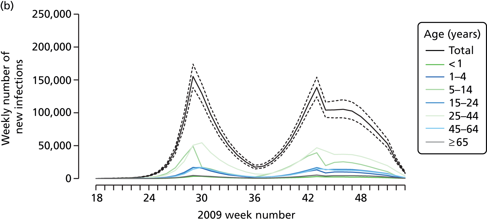
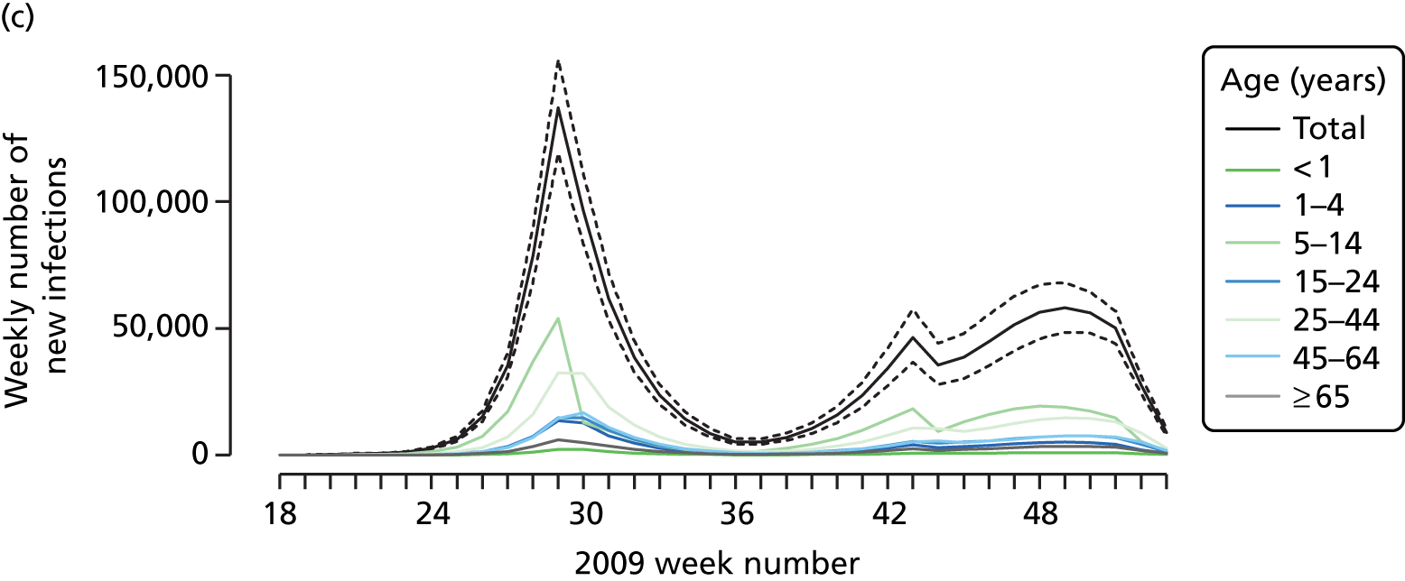
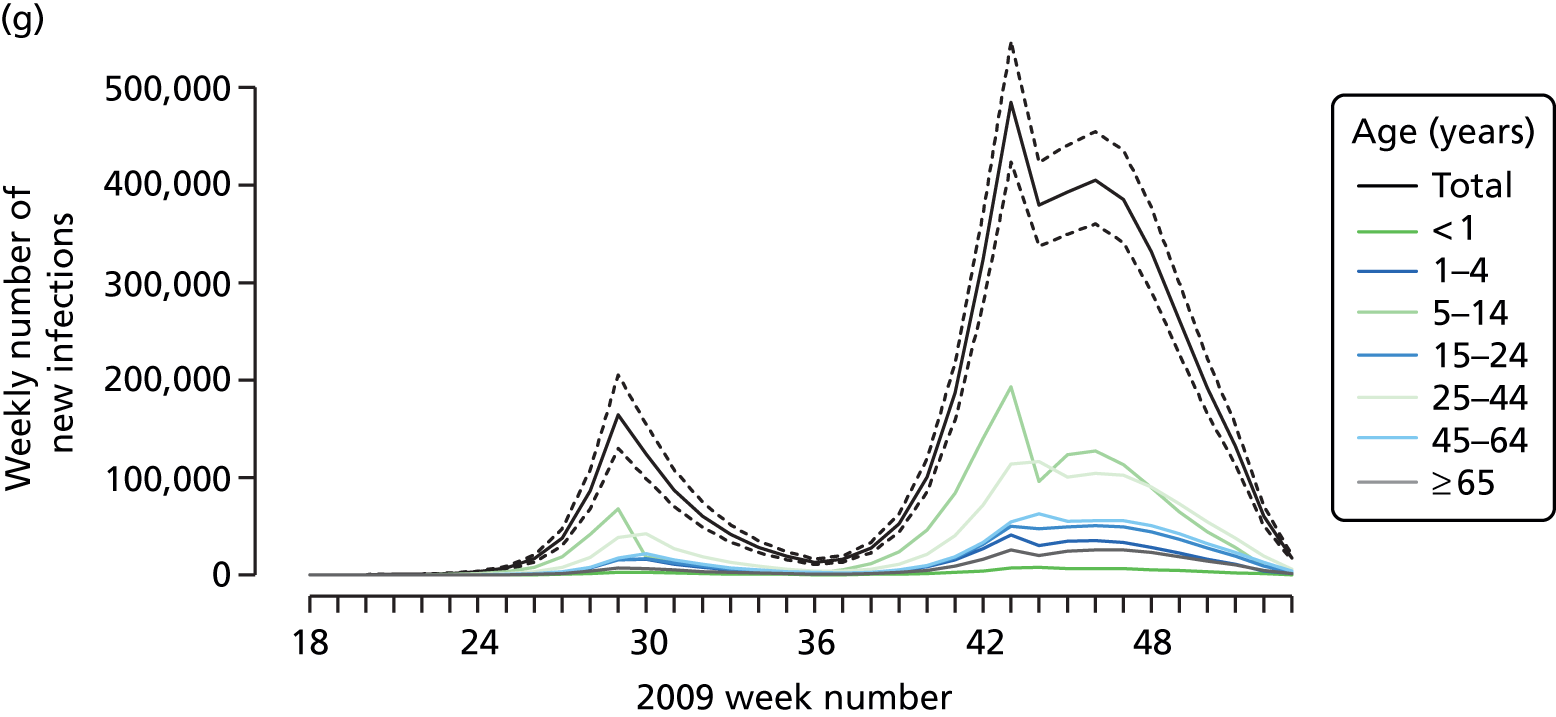
The PR and MR models are both sufficiently flexible to be able to reproduce the two epidemic waves of the 2009 pandemic. The estimated incidence curves are reproduced in Figure 3. The estimated epidemic in the North is consistent across both models. London and the West Midlands are characterised by bigger first waves of infection (and subsequently smaller second waves) under the PR model, the opposite being true for the South. This is apparent from the peaks in Figure 3 and the given population-level attack rates in Table 3 (age-specific attack rates can be found in Appendix 3). Peak timings in both waves of infection are the same under both modelling approaches, and coincide with the start of school holidays, with the exception of the second wave in the West Midlands. Here, a sufficient supply of susceptible individuals remains in the population after the holiday to allow transmission to increase once more (albeit briefly). This may well, however, be a phenomenon of different school term dates in this region to those that predominate elsewhere in the country.
FIGURE 3.
Estimated weekly number of new A/H1N1pdm infections for (a) London under the PR model; (b) London under the MR model; (c) the West Midlands under the PR model; (d) the West Midlands under the MR model; (e) the North under the PR model; (f) the North under the MR model; (g) the South under the PR model; and (h) the South under the MR model. Solid black lines represent incidence aggregated over age groups with associated 95% (CrIs) (dashed lines). Reproduced from Birrell et al. 28 © 2016, Macmillan Publishers Limited. This work is licensed under a Creative Commons Attribution 4.0 International License. The images or other third party material in this article are included in the article’s Creative Commons license, unless indicated otherwise in the credit line; if the material is not included under the Creative Commons license, users will need to obtain permission from the license holder to reproduce the material. To view a copy of this license, visit http://creativecommons.org/licenses/by/4.0/.




| London | West Midlands | North | South | |
|---|---|---|---|---|
| Parallel-region model | ||||
| May–August | ||||
| Infections | 988 (958 to 1124) | 525 (456 to 600) | 1058 (839 to 1316) | 692 (554 to 854) |
| Cases | 152 (123 to 184) | 80 (65 to 98) | 161 (121 to 215) | 105 (80 to 139) |
| Attack rate (%) | 13.2 (11.4 to 14.9) | 9.8 (8.5 to 11.2) | 5.6 (4.4 to 6.9) | 3.6 (2.9 to 4.5) |
| September–December | ||||
| Infections | 764 (641 to 901) | 571 (483 to 656) | 3671 (3379 to 3987) | 3750 (3508 to 4021) |
| Cases | 117 (91 to 153) | 87 (64 to 115) | 563 (462 to 689) | 576 (471 to 697) |
| Attack rate (%) | 10.1 (8.5 to 11.9) | 10.6 (9.0 to 12.2) | 19.3 (17.8 to 21.0) | 19.6 (18.3 to 21.0) |
| MR model | ||||
| May–August | ||||
| Infections | 751 (674 to 832) | 669 (621 to 718) | 886 (792 to 986) | 1150 (1036 to 1270) |
| Cases | 85 (74 to 98) | 76 (66 to 88) | 100 (87 to 117) | 130 (113 to 151) |
| Attack rate (%) | 9.9 (8.9 to 11.0) | 12.4 (11.5 to 13.3) | 4.7 (4.2 to 5.2) | 6.0 (5.4 to 6.6) |
| September–December | ||||
| Infections | 1228 (1129 to 1331) | 477 (405 to 559) | 3923 (3721 to 4129) | 3450 (3256 to 3658) |
| Cases | 140 (114 to 172) | 54 (42 to 69) | 447 (377 to 532) | 393 (329 to 472) |
| Attack rate (%) | 16.2 (14.9 to 17.6) | 8.9 (7.5 to 10.4) | 20.6 (19.6 to 21.7) | 18.0 (17.0 to 19.1) |
Estimated epidemic characteristics
Table 4 presents estimates of some key transmission parameters under both models. There is a pleasing consistency across the modelling approaches in the parameter estimates. For example, estimates for the (initial) reproductive number R0init, derived from the exponential growth rates, are centred on 1.8, with the region-specific estimates of the PR model being tightly distributed around this value. This is in broad agreement with other estimates for R0 obtained from a review of 2009 pandemic transmission parameters,50 and a slight increase on what had been estimated for the single region version of the model. 15 In a similar (single-region) modelling study, much higher estimates for the R0 associated with the A/H1N1pdm virus have been derived, although this was over the course of a later third wave of pandemic infection occurring in the winter season 2010–11. 51 Similarly, the estimates for the other transmission parameters are robust to the model specification [note the overlapping nature of the credible intervals (CrIs) in Table 4]. In particular, parameter m1, which gives the down-weighting applied to all contacts involving adults, is estimated consistently to be in the range 0.57–0.62. Estimates for m3 indicate that the summer school holiday period reduced the rate of effective infectious contacts among the 5–14 years age group to below 3% of the school term-time figure. However, when averaged over all age groups, this represents a drop in R0init of between 43% (in London) and 50% (in the South). To compare, a Canadian study recorded a 28% drop in transmissibility during a similar school holiday period. 52 The reduction in the effective contact rates in the other school holidays, as measured by parameters m4 and m5 were neither as well estimated (note the width of the CrI attached to the estimates for parameter m4) nor did they indicate a similar reduction in the contact rates, the shorter duration of these holidays evidently causing a milder disruption to routine contact patterns. Estimates for the proportion symptomatic, ϕ, do appear to be rather low, although consistent across approaches and with an estimate of 11% based on a closely observed outbreak. 53
| Parameter | PR model, posterior median (95% CrI) | MR model, posterior median (95% CrI) |
|---|---|---|
| R 0 | – | 1.810 (1.770 to 1.840) |
| d l | 3.470 (3.350 to 3.590) | 3.460 (3.340 to 3.580) |
| ɸ | 0.154 (0.126 to 0.186) | 0.114 (0.098 to 0.134) |
| m 1 | 0.569 (0.536 to 0.605) | 0.618 (0.584 to 0.651) |
| m 2 | 0.901 (0.610 to 0.996) | 0.666 (0.265 to 0.740) |
| m 3 | 0.007 (0.000 to 0.032) | 0.006 (0.000 to 0.032) |
| m 4 | 0.167 (0.008 to 0.669) | 0.214 (0.004 to 0.909) |
| m 5 | 0.446 (0.341 to 0.557) | 0.411 (0.291 to 0.528) |
Comparison between meta-region and parallel-region modelling
In Table 5, the posterior mean deviance is used to discriminate between different formulations of the MR model (to be discussed further in Goodness of fit), comparing each formulation relative to the comparable PR model. In fitting these models, MCMC provides a sample of parameter values {θ(1), . . . , θ(n)}, from which the posterior mean deviance, Dm=−(2/n)∑j=1nlog(Lm(y1:K;θ(j))) can be derived, where Lm(·;·) indicates the likelihood under a specific model, m. Note that lower values of Dm are preferred. The discrepancy between the PR model and the best-performing MR model is 57.89. Owing to the regional variation permitted by the PR model in the estimation of R0init and I0, the PR model has six more parameters than the MR model. This improvement in deviance for such a small number of parameters suggests that the PR represents a significantly better fit to the data. This compounds the practical benefit of the PR model being markedly faster to implement; it is more suited to parallel computation and the calculation of R0* in Equation 20 of Appendix 1, requires the calculation of eigenvalues of (7 × 7) matrices rather than the (28 × 28) or (44 × 44) matrices required by the MR model.
| α | Density type | Seed type | Commuting | ΔD(θ) (SD) |
|---|---|---|---|---|
| 0.0 | By stratum | Nextgen | Random | 3890 (34.23) |
| 0.0 | By stratum | Nextgen | Fixed | 4376 (33.83) |
| 0.0 | By stratum | Empirical | Random | 4548 (31.53) |
| 0.0 | By stratum | Empirical | Fixed | 4949 (32.21) |
| 0.5 | By stratum | Nextgen | Random | 3025 (34.21) |
| 0.5 | By stratum | Nextgen | Fixed | 2241 (32.13) |
| 0.5 | By stratum | Empirical | Random | 3191 (36.65) |
| 0.5 | By stratum | Empirical | Fixed | 2269 (31.90) |
| 1.0 | By stratum | Nextgen | Random | 2770 (30.23) |
| 1.0 | By stratum | Nextgen | Fixed | 2466 (30.05) |
| 1.0 | By stratum | Empirical | Random | 2578 (29.43) |
| 1.0 | By stratum | Empirical | Fixed | 2359 (29.39) |
| 1.0 | By region | Nextgen | Random | 449.2 (27.60) |
| 1.0 | By region | Nextgen | Fixed | 437.9 (27.21) |
| 1.0 | By region | Empirical | Random | 170.1 (28.47) |
| 1.0 | By region | Empirical | Fixed | 166.4 (29.76) |
| 1.0 | By region | Hybrid | Random | 57.89 (27.20) |
| PR model | 0 | |||
Finding an optimal parameterisation
Inferences drawn from either the PR or the MR modelling approach are found to be sensitive to the precise form of the regression for the background rates of GP consultation. Because of this, it was important to implement submodels of Equations 9 and 10 in order to most appropriately characterise the changes in consultation behaviour over the pandemic period. Again, the posterior mean deviance was used to identify a preferred model. The real-time PR model was repeatedly implemented with the higher-order interactions systematically removed from Equations 9 and 10 in the hope of finding simplified regression models without incurring any significant loss of fit to the data. Additionally, some age groups and regions were paired together to cover gaps where data were too sparse to warrant the additional age/region effects. Under the PR model, the seemingly optimal choice for the regression model, and the one that has been used in the generation of all the results presented in this section, is:
with the rates in the North found to be equal to those in the South, Br,a(tk) = Bs,a(tk). This is unsurprising given the sparsity of virological data in the North to accurately estimate the non-pandemic consultation rates. Also, the rates in the two youngest age groups have been set to be equal (note the sum over the a index omits a = 1), Br,1(tk) = Br,2(tk), which, again, is not an unreasonable finding given that only the virological swabbing and not the QSurveillance GP data sets provide data with sufficient granularity to distinguish between the first two age groups (< 1 year and 1–4 years).
When the same model refinement process was undertaken using the MR model, the same regression equations were again preferred.
Having established the form of the regression equation for the background consultation rates, the next stage of model building in the MR approach was to consider the alternative model formulations of Chapter 3, The meta-region model, governing how the model handles density dependence, random commuting and the choice of the initial seeding. Examination of the posterior mean deviances presented in Table 5 shows that density dependence is best accounted for by scaling entries of the contact matrices by the population of the region, not the population of the relevant stratum, that is, by replacing Nr,a and Nv,a in Appendix 1, Equation 27 with Nr and Nv, the sum of the regional populations over age groups. Furthermore, it was found that within-region transmission that is density dependent (corresponding to the case α = 1 in Equation 27 of Appendix 1) gave better model fit than either frequency-dependent transmission (α = 0) or a mixture of the two (α = 0.5).
Meta-region model performance is highly sensitive to the choice of initial seeding of infectivity, with the hybrid seed performing most strongly. When the number of strata is expanded to partition between non-commuting and commuting adults, there was no consistent improvement in model performance (nor any particular worsening). However, the extra complexity and computation required to evaluate the model with the expanded number of strata indicates that the reduced stratification would be preferred in a real-time context. This suggests that the effects of inter-region transmission are either highly transient, sufficiently so that its effects are swallowed up by the choice of seeding, or the movement of individuals between regions is poorly characterised by the commuting data. The formulation of the contact matrices assumes that infected individuals move as freely as uninfected individuals, and this may well be unrealistic. However, accounting for this would further reduce any difference in model performance between the two approaches, and thus would not lead to any material adjustment of the conclusions.
All results presented that quote the MR model will refer to the best-performing variant with α = 1, density dependence governed by the regional population size, using the hybrid seed and assuming commuting at random.
Goodness of fit
Appendices 3 and 4 give goodness-of-fit plots for three of the data types (GP consultation data, virological positivity data and serological data) under the PR and MR models respectively. There is no apparent lack of fit under either model, with most data points lying within the 95% predictive intervals. In a couple of instances the seropositivity predicted by the model is too high (Greater London, ≥ 65) and in others too low (Greater London 5–14). It would seem that this is due to poor estimation of the initial proportion of susceptible individuals (this is an a priori estimation, it was not carried out as part of the real-time model effort). Even in these cases, the PR model gives the better fit to these outlying data points, with fewer points missing their predictive intervals. Elsewhere, the performance of the PR model is evidently superior, in accordance with the findings already presented.
Comparison of the real-time performance of the Monte Carlo methods
The results in section Spatial modelling were all obtained using MCMC. A posterior sample from the PR model could be derived in about 13–15 hours, with some parallelisation of the likelihood. The MR approaches took considerably longer, particularly under the fixed commuter assumption when there were 44 population strata. At this point, the run-time stretches into days. Even at 13 hours, however, this is longer than a typical working day and eliminates the possibility of providing real-time analysis. Furthermore, it is not yet considered that in any future pandemic there should be a sufficient wealth of data to allow a greater subdivision of England, at least into the nine GORs, or that the improved quality of surveillance data might lead to an expansion in the number and type of parameters that can be estimated. Alternatively, the next pandemic to occur might be longer lasting, giving longer time series of data. All of these factors can greatly increase the level of computation required to draw the required statistical inference. It is not desirable that estimates are rendered obsolete by new data before they can be produced.
This highlights the importance of developing a good statistical algorithm for analysing the data in a timely fashion. The algorithm also has to be able to be expressed in sufficient generality that it can be encoded within software for future use by an infectious disease epidemiologist whose knowledge of computational techniques in statistics may be minimal. As alluded to in Chapter 1, there is reason to believe that SMC algorithms may permit the iteration of analysis in a much more timely fashion. In this section, the efforts to tailor a suitable yet reasonably general SMC algorithm are discussed, testing the approach against simulated data, the generation of which is described in what follows. The central idea is that the data should be realistic, yet have features that are challenging to track, a ‘worst-case’ scenario from a modelling perspective.
Simulated data
It was decided to copy many of the features of the 2009 pandemic. The simulated outbreak starts with an initial burst of infections in the spring, so that the epidemic is in full exponential growth by the time of an over-summer school holiday. The school holiday acts as a break on transmission, partitioning the outbreak into two distinct waves of infection. Although we only consider this one underlying epidemic, we consider two different data scenarios. In the first scenario, it is assumed that there is direct information on confirmed cases, such as might occur in the surveillance of severe disease (e.g. hospitalisation or ICU data from USISS). In the second scenario, ILI consultations, contaminated by non-pandemic infections replace the confirmed case data. Both data streams are assumed to exist alongside serological data. In the second scenario, it is necessary to have companion virological swabbing data to identify the degree of contamination in the ILI data.
To ensure that the task of epidemic tracking is realistic, in the same vein as the NPFS introduction in 2009, it is assumed that there is a ‘shock’ in the data provided by the surveillance schemes. Such a shock would be provided by a public health intervention designed to alleviate overcrowding in primary health-care services or to reduce the demand on hospital beds. The net result of the intervention is that a much reduced proportion of cases report their symptoms to the respective surveillance schemes, with the timing of the intervention, as in 2009, following shortly on from the over-summer closure of schools for the holiday period.
To illustrate the size of the system shock that is being considered, the synthetic data to be used in the second scenario are presented in Figure 4.
FIGURE 4.
Synthetic data generated to test the SMC algorithms. Top row: (a) observed number of GP consultations; and (b) swab positivity data with numbers representing the size of the weekly denominator. Bottom row: (c) serological data; and (d) the pattern of background consultation rates for the GP consultation data aggregated over ages. The green arrows over figures (a) and (c) highlight the timing of some key, informative observations.

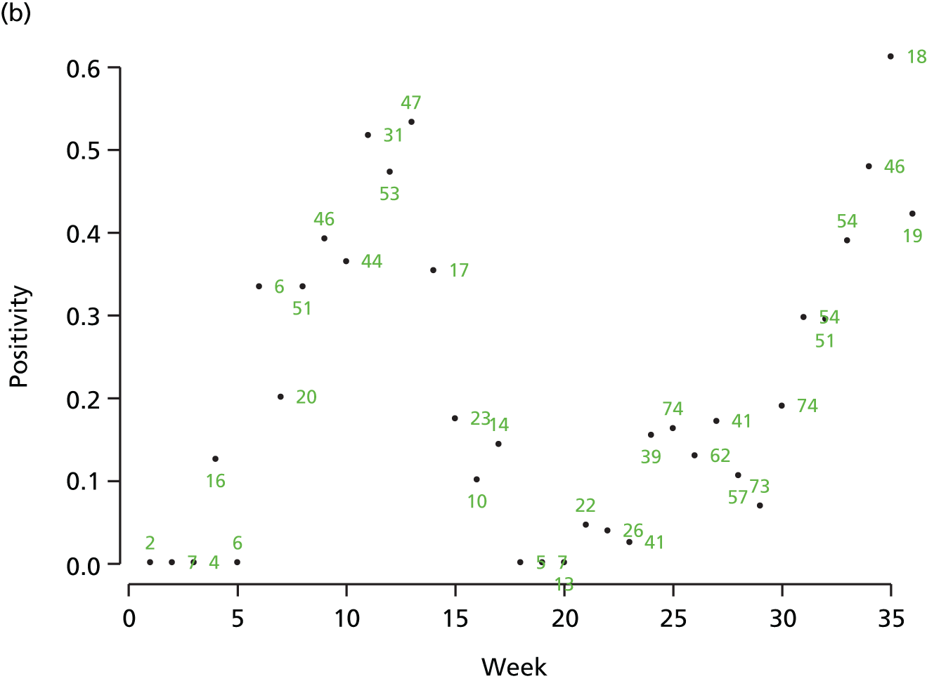


Scenario 1: a naive algorithm
Here, we want to compare the relative performance of the SMC algorithm against what we consider to be a gold standard, the MCMC algorithm that was used to derive epidemic inference in earlier analysis of the 2009 data. 15
To attempt this, MCMC analyses are carried out after 50, 70, 83, 120, 164 and 245 days of data have been observed. The SMC algorithm was then applied starting from the MCMC-derived posterior from 50 days, to see if, after the addition of 20 consecutive days, or batches, of data, the SMC and MCMC derived posteriors are statistically similar. This process was repeated to see if SMC could also bridge the gap between the MCMC analyses at days 70 and 83, days 83 and 120, days 120 and 164, and days 164 and 245.
Initially, a fast, naive SMC algorithm was tried in application to the first data scenario, where we have contamination-free hospitalisation data. Here, the MCMC step embedded within the SMC algorithm would only last for one iteration, and rejuvenation of the particle set would only take place after the assimilation of whole batches of data (none of the fractional addition of data discussed in the When to rejuvenate? When are the particles degenerate? discussion in Chapter 3, Sequential Monte Carlo). Figure 5 shows some of the results. In the scatter plots, the light green points show the starting MCMC-obtained distribution. Against this, left-hand scatterplots are to be compared with the right-hand scatterplots. On the right-hand side, all scattered points (except the light-green points) are of the same colour, because they are all of equal weight and of equal importance. In the left-hand column, the darker the point, the greater weight it carries.
FIGURE 5.
Comparison of naive SMC (left-hand-side panels) and MCMC (right-hand-side panels) at (a) tk = 70 days, (b) tk = 120 days, (c) tk = 245 days, via scatterplots for the parameters ψ and υ.
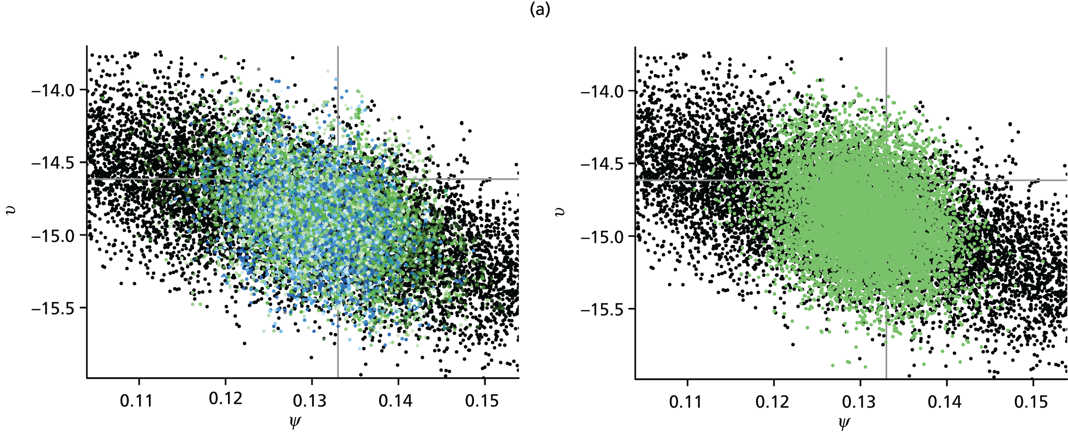
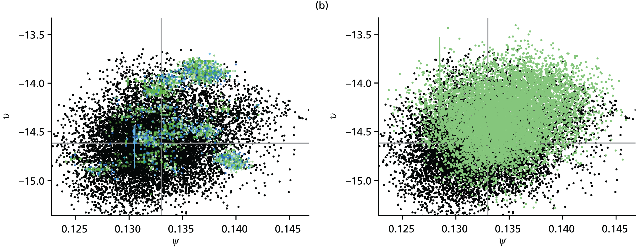
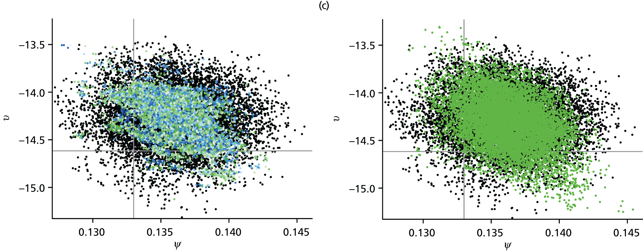
The immediate point to notice is that the SMC-obtained posteriors in the top and bottom panels would appear to be comparable to the MCMC-obtained posterior distributions, but the posterior distribution obtained by the naive SMC algorithm at time tk = 120 displays significant degeneracy. The algorithm has not tracked the movement of the posterior density over the interval from 83 days to 120 days. It is this sample impoverishment that makes the naive SMC inefficient at such a time.
Referring to the plots of the simulated data in Figure 4, the superimposed vertical green arrows identify points in time where there are particularly informative observations. Immediately after time tk = 83, there is a shock to the surveillance system as a public health intervention diverts people away from GP surgeries, drastically cutting the proportion of infections that are reported in the data. At time tk = 110, there is a particularly large batch of serological data that are particularly informative. These two occurrences make it particularly hard for the naive algorithm to track the epidemic. Particularly after the tk = 83 days shock, a number of new parameters become active (i.e. begin to have influence over the likelihood). As parameters first begin to move away from their prior density, it can cause severe depletion of the particle set. In comparison, the 50–70 day and the 164–245 day intervals are relatively uneventful and much easier for the algorithm to track.
It is this phenomenon that motivates a focus on the day 83 to day 120 interval moving forward, and also motivated the algorithmic adaptations discussed at the end of Chapter 3, section Sequential Monte Carlo. We also consider the second data scenario, where syndromic GP counts, inclusive of non-pandemic noise and virological swabbing data are available.
Scenario 2: heavy-duty sequential Monte Carlo
If the MCMC-derived posteriors are to be treated as a (albeit computationally costly) gold-standard, a measure of similarity is needed between the SMC- and the MCMC-derived distributions, and for this we use Küllback–Leibler (KL) divergence. 54 This is a statistic that gives a measure of how different an estimate for a probability distribution is to its ‘true’ target. Here, we are presuming that it is the MCMC that represents the truth.
Table 6 gives the KL statistics achieved when the full SMC algorithm was used over the day 83 to day 120 interval, breaking the interval down even further so we can look at KL discrepancies in the immediate aftermath of the shock at tk = 83 days. The table also shows three different levels of ICC threshold used as a stopping criterion for the MCMC phase. At each time, the ‘gold standard’ MCMC analysis was repeated numerous times and then referred back to a reference analysis. This was done to build up a distribution of KL statistics, so that the SMC analysis could be given a KL ‘target’, the upper 95 percentile of the KL statistics calculated on the sample of MCMC analyses. If the SMC analysis had a KL statistic that was lower than the target value, then it could be said to be indistinguishable from the MCMC analyses. At this point, we know that the SMC algorithm is responding adequately.
| Time point | ICC threshold | ||
|---|---|---|---|
| 0.5 | 0.2 | 0.1 | |
| 84 days (KL target = 0.732) | 2.92 | 2.87 | 2.83 |
| 85 days (KL target = 0.135) | 3.05 | 3.00 | 2.98 |
| 86 days (KL target = 0.365) | 3.28 | 3.24 | 3.25 |
| 87 days (KL target = 0.276) | 2.54 | 2.45 | 2.42 |
| 90 days (KL target = 0.159) | 1.80 | 0.353 | 0.0663 |
| 100 days (KL target = 0.135) | 0.157 | 0.102 | 0.0890 |
| 110 days (KL target = 0.122) | 0.159 | 0.0774 | 0.111 |
| 120 days (KL target = 0.119) | 0.136 | 0.0435 | 0.0708 |
From Table 6 it can be seen that, from about day 87 onwards, the SMC algorithm (for the ICC thresholds 0.1 and 0.2) begins to regularly hit its KL target. The problem, therefore, lies in the days immediately preceding this point in time, where, not only are the KL statistics large, but the MCMC-component of the SMC algorithm requires vast numbers of iterations and becoming prohibitively time-consuming.
Addressing the speed issue first, it was found that one particular parameter was causing the slow convergence. As discussed elsewhere,47 it was found that, if proposals for the overdispersion for the negative binomial data η were made separately to the rest of the parameter vector θ (which is updated together in one block), convergence could be achieved much more rapidly. Figure 6 shows the improvement in the number of iterations required per day from over 400 per particle under the original SMC algorithm to 70 under the tailored version on day 89, with this improved performance evident for a number of days in the aftermath of day 83. Under both schemes, rejuvenations are required at the same times, but do not require the same computational effort. Both versions of the algorithm perform similarly from around day 90–91 onwards.
FIGURE 6.
Computational demands of the SMC algorithm. (a) Number of MH steps required by the continuous-time SMC algorithm per rejuvenation against the timing of the rejuvenation for both the continuous-time algorithms (black and green correspond to with and without η in the block updates) with the ICC threshold = 0.1 (solid line), 0.2 (dashed line) and 0.5 (dotted line). (b) Total number of MH steps required by the continuous-time SMC algorithm per time interval with ICC threshold = 0.1 and with (black bars) and without (green) η in the block updates.


This simple tailoring of the algorithm, only really necessary while a parameter is only weakly informed by the data and has an uninformative prior attached to it, evidently speeds up the algorithm, but it is necessary to show that this causes no degradation in terms of the inference that can be gathered. Table 7 repeats the exercise of Table 6, showing performance that is almost identical over the period 84–87 days (inclusive), the period over which there is a substantial speed-up in the implementation of the algorithm. Thereafter, for the thresholds 0.2 and 0.1 the performance is comparable to MCMC, with the exception of what appears to be an anomalous reading for the 0.1 threshold at 90 days.
| ICC threshold | 0.5 | 0.2 | 0.1 |
|---|---|---|---|
| 84 days (KL target = 0.732) | 2.97 | 2.85 | 2.86 |
| 85 days (KL target = 0.135) | 3.06 | 2.97 | 2.98 |
| 86 days (KL target = 0.365) | 3.27 | 3.22 | 3.26 |
| 87 days (KL target = 0.276) | 2.51 | 2.48 | 2.44 |
| 90 days (KL target = 0.159) | 2.10 | 0.0927 | 1.42 |
| 100 days (KL target = 0.135) | 0.107 | 0.0835 | 0.0701 |
| 110 days (KL target = 0.122) | 0.197 | 0.0373 | 0.0348 |
| 120 days (KL target = 0.119) | 0.0999 | 0.0423 | 0.0551 |
However, the failure of the algorithm to hit the MCMC thresholds over the interval 85–87 days (and 88, 89 days also, not shown) is a concern, and motivates an examination of scatterplots akin to those of Figure 5. In Figure 7 we look at scatterplots of the MCMC- and SMC-derived posterior distributions for two regression parameter components of the non-pandemic ILI consultations, βB. The MCMC plots are comparable to the SMC-derived plots immediately to their left. What they show is that, most strikingly on the 84–85 day and the 85–86 day steps, the MCMC algorithm is not capable of the same coverage of the space that the SMC algorithm achieves. This is a result of poor convergence of the MCMC algorithm. It gets stuck within a smaller range of values. It may be that the MCMC algorithm needs many more iterations to properly sample the full range of values, but it is already at a considerable computational disadvantage (typical runs are of chains of length 750,000 iterations).
FIGURE 7.
The evolution over time of the marginal joint posterior for two components of the parameter vector βB, comparing SMC-obtained (left-hand-side panels) and MCMC-obtained (right-hand-side panels) posterior distributions. Light-green points indicate the distribution at the start of the interval. (a) 83–84 days; (b) 84–85 days; (c) 85–86 days; (d) 86–87 days; (e) 87–90 days; (f) 90–100 days; (g) 100–110 days; and (h) 110–120 days.
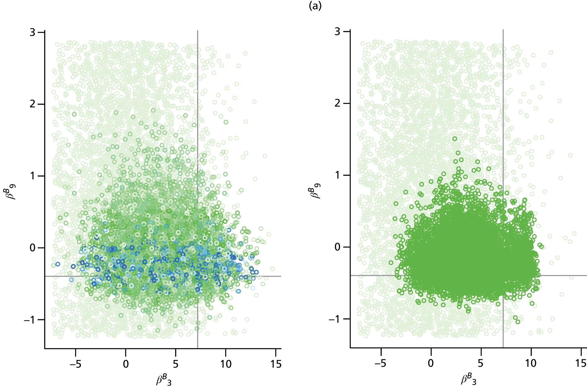


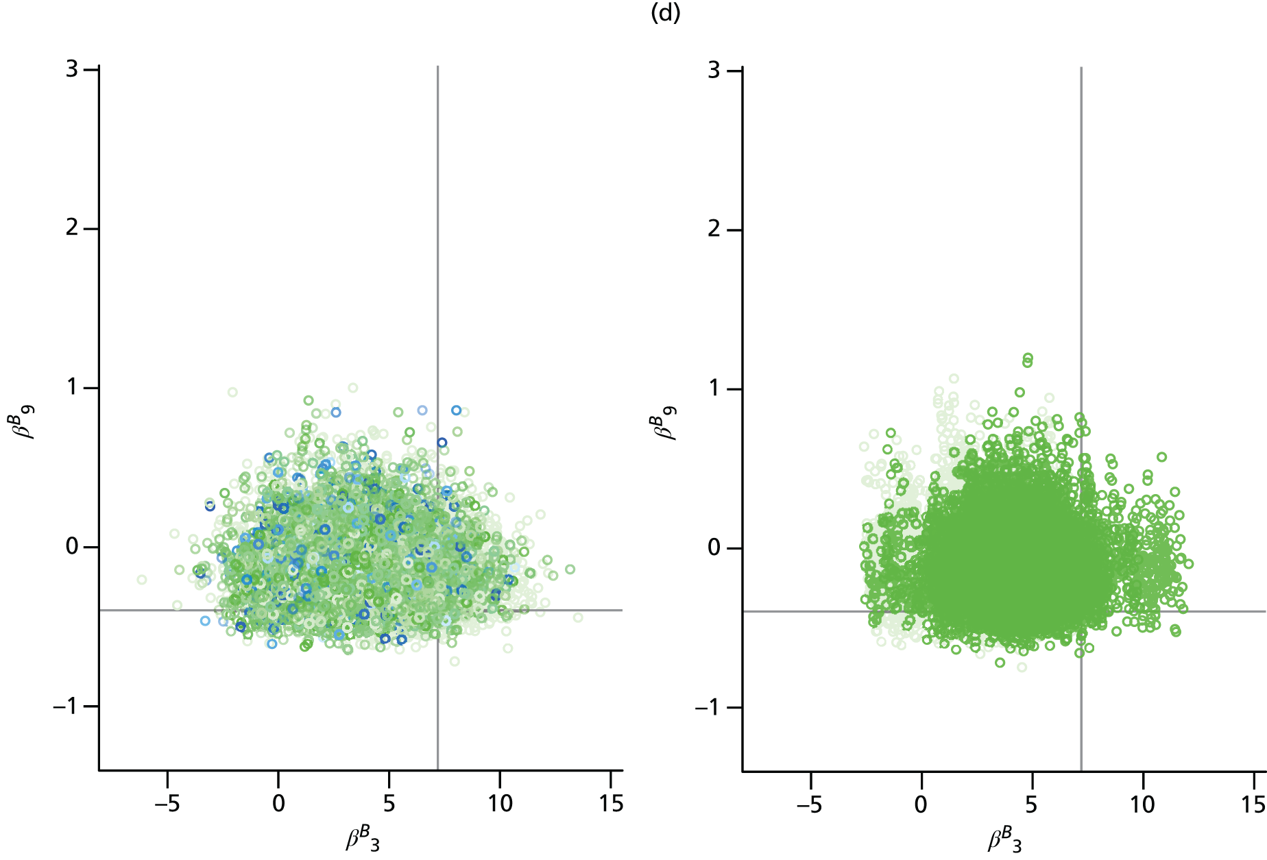


There is, therefore, a strong suggestion that the MCMC analysis, far from being a gold standard, is actually inferior to the SMC analysis. Where Table 7 seemingly shows the supposed inability of the SMC to provide a posterior sample that could be considered representative of the MCMC sample, this may actually be a result of the weakness of the MCMC algorithm, and SMC is preferred.
Returning to Figure 6, on the arrival of the data from day 84, each particle can be seen to require 220 iterations to accurately transition to a suitable posterior sample. When considered across 104 particles, this represents a number of evaluations of the full likelihood that is less than four times that which is required by the 750,000 iterations of the MCMC algorithm typically used to derive a sample. As multiple chains are typically required to correctly diagnose convergence and to provide a sample, it can be seen that the SMC would only require only very modest benefits from parallelisation to be quicker to compute. When placed on a computing cluster, the SMC is considerably quicker to implement. The SMC algorithm developed here was implemented on a cluster that, depending on availability, permitted simultaneous calculation on 100 + processors. The particles are distributed evenly across the available processors, so that calculations on many particles are ongoing in parallel. Only at the resampling step and in the calculations of the ESS and the ICC is information shared across the processors. At day 83, we are considering the batch of data for which the greatest computational effort is required for the SMC analysis to derive inference. Elsewhere, the computational benefits of SMC are more clearly observed (e.g. by the end of the 83- to 120-day interval, less than 10 iterations are required for rejuvenations). For batches of data that do not lead to a rejuvenation of the particle sample, the SMC updates require a negligible amount of time to compute and are evidently very much quicker than the MCMC analyses, which still have to run very long chains to produce a reasonable posterior sample.
Chapter 5 Discussion
Achievements and objectives
The objective of this work was to advance the state of the art of real-time modelling of influenza epidemics and to provide a tool that could be used to monitor and predict the development of an ongoing pandemic outbreak.
We have advanced the state of the art by:
-
Developing transmission models that account for spatial heterogeneity in the spread of infection.
-
Improving the efficiency with which the estimation and prediction of an epidemic can be carried out, through the development of a SMC algorithm that will greatly reduce the computational burden for routine data analysis as part of a programme of pandemic surveillance.
-
Facilitating the ability of the public health community to provide timely online inference to policymakers through the provision of software to implement both of the above. The software has been adapted for the anticipated suite of epidemic data, and key PHE scientists are engaged with ongoing training in its use. The computing code (and any related documentation) for the MCMC and SMC implementations of the real-time model are stored in open online repositories. 55,56
In the initial proposal, there was also a component of this research promising support to the HPA (now PHE) in the event of a pandemic outbreak during the scope of this grant, in their real-time production of estimates and projections of the health-care burden attributable to the pandemic. Such an outbreak did not occur, and thus this component of the project has not yet been activated.
Strengths and limitations
Spatial modelling
This work has led to a coherent, unified, Bayesian statistical analysis of multiple streams of epidemic surveillance data from the 2009 A/H1N1pdm outbreak in England, producing age and region stratified epidemic reconstructions (with associated uncertainty) and robust estimates of the parameters of the transmission process. We have explored two modelling approaches: the PR and the MR models. Both fit adequately well the various data sources, with highly comparable estimates for both model parameters and epidemic characteristics that are consistent with existing literature.
Each approach has its strengths and limitations.
The PR approach is found to be parsimonious, yet sufficiently flexible to capture the underlying dynamics. It is also ‘non-parametric’, in the sense that the parameters representing the epidemic growth and initial seeding of infectiousness in each region are estimated without being subject to any parametric assumption. The assumed lack of relation between these parameters means that the spread of infection between regions cannot be forecast, and significant epidemic activity has to be observed in all regions to enable estimation of the epidemic burden. This lack of predictive ability is a limitation in the use of the PR approach. However, the greater flexibility becomes an advantage when it comes to epidemic reconstruction, and this is observed in a significant improvement in the model fit of the PR approach to the 2009 pandemic data. An additional advantage is that this modelling approach does not rely on the validity of the commuter data to describe the spread of infection, nor does it rely on the assumption that individuals maintain routine commuting behaviour regardless of infection status. Despite the permitted spatial variation in epidemic growth rates, the PR model provides estimates for R0init that are consistent across regions. Therefore, the spatial heterogeneity in infection is being accounted for through the initial seeding of infectiousness.
The MR model incorporates spatial heterogeneity in transmission, arising from the interaction between regional populations, through commuting flows. This gives the MR model greater power to predict the spatial spread of influenza, enabling the prediction of which will be the next region to experience widespread infection. Early in a pandemic, therefore, the MR approach is more useful in a predictive modelling setting. However, it has been seen elsewhere that long–range interactions have a declining role in the spread of a pandemic once infection is widespread in each region. 57 This is exacerbated for A/H1N1pdm influenza as school-age children, the demographic group most affected, do not contribute to commuter movements. This marginalises, to some degree, the key benefit of this approach. Additionally, the MR approach involves an increased computational burden that limits its use as a tool for timely epidemic tracking as data accumulate over time.
One variant of the MR model investigated here involved the stratification of the population within each region into commuters and non-commuters. This has the effect of assuming that each region contains a fixed subpopulation of individuals who commute daily. This formulation yields no consistent improvement in model performance, while further increasing the computational cost. Factoring in the ‘random’ movements of casual and occasional travellers, who have been quoted to potentially increase the rate of transmission between regions by 25%,58 would involve further computational burden, and is particularly difficult to implement in an inferential setting without appropriate auxiliary information (e.g. if the census data contained information on the purpose of travel).
The MR model could be made more realistic and detailed by assuming that a proportion of those with symptomatic illness may not travel, or that asymptomatic illness is less infectious. However, consideration of such factors would only lessen the contribution of long-range transmission, leaving the conclusions unchanged.
To summarise, using a Bayesian statistical framework the PR model is found to be sufficiently flexible to provide a good fit to data, is quick to implement as it includes lower-dimension contact matrices, and the non-interacting nature of the regions means that the likelihood calculations can be easily parallelised. Reassuringly, it also provided concurring estimates for the basic reproductive number (R0init) across the regions, in agreement with the MR approach. However, the PR model can provide little insight into inter-region transmission and the determinants of spatial heterogeneity in the spread of infection because of its simple structure. In a situation where school-age children are the main agents of transmission and baseline transmissibility is not high, spatial models that concentrate on local transmission, like the PR model, provide a powerful and timely tool for use by public health services, helping to inform effective control and containment measures.
Efficient estimation and prediction
We have proposed addressing the substantive problem of real-time tracking of an emergent and realistic epidemic, assimilating multiple sources of information through the development of a suitable SMC algorithm. When incoming data are stable, this process can be automated using standard algorithms in line with approaches already in the literature. 12,27 However, in the presence of interventions or any other event that may artificially interrupt the epidemic’s trajectory or even result in a shock to the epidemic system, it is necessary to adapt the algorithm appropriately. How the algorithm is adapted will depend on the scale of the disruption to the surveillance data. The end result is a semi-automated SMC algorithm that can be tailored to the nature of the shock to limit the required computation time.
This hybrid SMC can be seen to greatly outperform MCMC when it comes to successively iterating analyses, as will be required in a pandemic scenario. Throughout, we have compared the divergence between SMC posteriors from posteriors generated by the ‘gold standard’ MCMC. However, this may be an unfair comparison, as the MCMC algorithm is based on ‘plain vanilla’ Metropolis updates, and could benefit from an in-depth tuning process itself. More sophisticated MCMC algorithms could be used, for example differential geometric MCMC or parallelised MCMC. 59,60 These could assist with improving MCMC run times. On the other hand, as MCMC steps are the main computational overhead of the SMC algorithm, any development of the MCMC algorithm may also lead to similar improvement of the SMC algorithm. It is also worth adding that the benefits of SMC for real-time analysis have been demonstrated. For a single, one-off, analysis aimed at reconstructing the epidemic dynamics, the SMC algorithm would be implemented differently and may not hold any significant advantage over MCMC.
Finally, the analyses carried out in this work have neglected the first 50 days of the epidemic, concentrating on a period when there is substantial transmission in the population and appropriate data are becoming available. As a result, a deterministic system can adequately describe the future evolution of the pandemic. Stochastic effects are significant and need to be incorporated into the model if monitoring is needed in the earlier stages. A prescription exists for what is known as ‘particle learning’ in the presence of ‘shocks’ in such a setting. 61 Alternatively, to improve the robustness of the inferences, the piecewise linear quantities describing population reporting behaviour could be described by linked stochastic noise processes. This has the potential to reduce the sensitivity of estimates to the presence of change points that are not, for whatever reason, foreseeable.
Over the course of this project, the state of the art of statistical computing in epidemic models has advanced in many directions, motivated by influenza and also by recent Ebola outbreaks. 11,27,62–64 Each approach, however, uses direct observations of cases or estimates of cases to fit models. It is believed that our approach to tackling a realistic, messy suite of epidemic data is both novel and critically important.
Pandemic data
The capacity to provide real-time estimation and prediction of an epidemic is not only dependent on the existence of models and software. Crucial to this ability is the richness of the available public health surveillance data and its timely availability. The UK is well served in terms of the depth and completeness of its influenza surveillance mechanisms, and the timely availability of data can be almost guaranteed whenever it arises as a result of routine collection and reporting. This is not quite the case for the serological information, however, which requires suitable tests to be developed, and samples to be collected and analysed. The role of serological data is shown in figure 10 of Birrell et al. ,47 in which epidemic projections have been sequentially made using only noisy primary care consultation data in the absence of serology data. A reliable picture of the epidemic is not available until the epidemic is almost over. This poses some key questions: are serological samples going to be available in a timely manner, in sufficient quantity and quality, and in the right format? The availability of this data is a potentially limiting factor.
Routine influenza surveillance data may be reliable in terms of its timely provision. However, such data may become unreliable as infection becomes more widespread and the demands placed on health-care services increase. Hospital beds and GP appointments are finite, and the health-care system may be operating at capacity for a period. Services such as NPFS are designed to alleviate this burden in primary care, but, in particular, we have to entertain the possibility that the proportion of cases that lead to hospitalisation might artificially diminish. The model will permit time variation in ph to account for these density-dependent effects, but how to diagnose and characterise this decline are still open problems. As will be discussed in Chapter 6, section Alternative influenza-like illness surveillance, this motivates an exploration of the relationship between primary care ILI surveillance and community ILI surveillance. The aim is to find alternative data sources whose interpretation and collection is robust to high levels of influenza activity and can, therefore, constitute a valuable addition to the array of data already under consideration.
Chapter 6 Conclusions
Research recommendations
There are a number of very evident areas for future research and we summarise them briefly in the following sections.
Alternative influenza-like illness surveillance
The majority of ILI presentations to health services will be via primary care, at least up to a point at which a service such as the NPFS is initiated. There are a number of potential additional surveillance systems that capture ILI occurring in the community, for example telephone calls to the NHS 111 service, GP out of hours, and RCGP spotter practices. 65 Once NPFS is activated, most ILI presentations will be diverted to this service, with integrated self-sampling providing data on virological positivity. The model currently works with GP ILI diagnoses reported via GP in-hours. There is the potential to use an amalgamation of the available surveillance data. If this were to be considered desirable, then further research would be required to understand the overlap between the systems, as well as to understand how to measure virological positivity under each of the schemes.
As discussed in Chapter 5, section Pandemic data, the reliability of the data from traditional ILI surveillance schemes diminishes as resources become more stretched. This may motivate the potential use of alternative surveillance mechanisms that are not reliant on the allocation of health-care resources. These could be through internet searches,66 social media data,67 community reporting of symptoms44 or even sales of thermometers. 68 How to integrate these types of data into mechanistic models for disease transmission is still little understood and warrants further investigation.
Incorporating interventions
To improve their utility as an epidemic response tool, the models presented here should be developed further to account for any interventions and mitigation strategies that may be employed during an influenza pandemic. Any intervention deployed and strategies used will depend on the nature and severity of the outbreak,69 although they fall into two categories: pharmaceutical interventions (e.g. antivirals, antibiotics and vaccinations) and non-pharmaceutical interventions (e.g. school closures and hygiene campaigns).
The use of a pandemic specific vaccine would occur a few months after the start of the pandemic once a vaccine had been developed and manufactured. Vaccination has the effect of changing the state of a substantial proportion of those vaccinated, the size of which would be dictated by the vaccine efficacy, from ‘susceptible’ to ‘recovered’, making the vaccinated individuals bypass other states within the model. Accounting for vaccination would then require a modification to the transmission model structure to enable the flow of vaccinated individuals directly between ‘susceptible’ and ‘recovered’ model states. This flow would be informed by external data on vaccine coverage and vaccine efficacy.
A mitigation strategy that has been extensively studied is that of closures of schools. This strategy can be incorporated directly into the current model in a manner similar to how the model currently handles school holidays, that is, by manipulating entries of the contact matrix corresponding to school-age children. There are several studies that have estimated the changes in contact patterns during school holidays. 70 However, prolonged school closures may lead to wider differences in contact patterns that, to our knowledge, have not been rigorously studied. Further research may well be required to inform how the contact matrix would differ from that of school holiday periods.
Other non-pharmaceutical interventions can be used to slow the spread of infection and buy time for the development of biomedical interventions. These interventions may include hand-hygiene campaigns and advice to avoid large gatherings, and they go hand in hand with other events that may influence the public’s response to the pandemic, such as high-profile illnesses and sensationalist media reporting. These can impact on transmission, but perhaps more significantly from a modelling perspective, they can influence how people interact with health-care services and report their illness, directly affecting the data used in the modelling. Therefore, developing an understanding of these behavioural changes in real time is vital to be able to accurately estimate the scale and spread of infection and the attached uncertainties.
Stochastic model adaptations
As noted in Chapter 5, section Efficient estimation and prediction, the existing modelling approach only has utility once the epidemic is well established and the infection is widespread. A consequence of this is that it is difficult to say anything about the early stages of the pandemic with any degree of certainty, and parameters describing initial conditions of the dynamic transmission model have no real interpretation. Recent work by Shubin et al. 71 implements a similar model to Birrell et al. 15 to reconstruct the Finnish pandemic in 2009, with the exception that stochastic dynamics are used. Introducing similar stochastic dynamics in our spatial models would be of some interest, particularly in the MR modelling where the pattern of inter-region transmission would be less rigidly defined by the commuting data. A further aspect that could be improved through the injection of stochasticity is the robustness of inferences. For example, parameters depending on the health-care-seeking behaviour of populations could be replaced with stochastic noise processes. Such processes could take the form of the endemic/epidemic model,72 for example, and would remove the sensitivity of the estimated epidemic trajectories derived by the pandemic model to the choice of changepoints discussed in Chapter 5, section Efficient estimation and prediction. Furthermore, these processes are sufficiently flexible to incorporate any information on external factors that may influence the health-care-seeking behaviour of a population.
Timely provision and understanding of serological data
The role of timely serological data has been demonstrated for the 2009 pandemic. As will be discussed in Implications for health care later in this chapter, it is vital that a system should be in place that can be exploited promptly in the event of a pandemic to give reliable information on susceptibility to the pandemic strain both at the beginning of and throughout an epidemic.
However, it is possible that too much weight has been attributed to these data. Immunity is assumed to be present in all individuals with haemagglutination inhibition assay titre values above a given threshold, but in reality, things may not be quite so well defined. It would be ideal if the uncertainty in determining the presence of immunity could be propagated into the analysis of the real-time model. This has been done in an analysis of Dutch A/H1N1pdm data, where protein microarrays were used as a diagnostic assay to investigate antibody responses in cross-sectional serological samples. 73 This provided a probabilistic statement of whether the individual was susceptible, was recently infected or held long-standing immunity. Being able to incorporate this type of information into the analysis would improve the handling of uncertainty in the model and give a clearer picture of initial levels of susceptibility.
Routine operation
Each autumn/winter there is an annual influenza season over which rates of infection are heightened. Each season is characterised by a unique blend of circulating influenza viruses, leading to illness of varying severity. Typically, the well of immunity in the population to the circulating viruses prevents an escalation to pandemic levels. However, these seasonal infections exert a health-care burden, and models could inform the estimation and prediction of this burden. Routine operation of the real-time modelling system during these seasonal outbreaks ahead of a possible pandemic would provide invaluable insight into algorithmic performance, would allow PHE epidemiologists to familiarise themselves with the software and epidemiologists to become familiar with the model’s data requirements. Both could then formally be involved in the change process whenever the model requires adaptation in light of any unforeseen operational hitches that may be identified as the relevant surveillance schemes evolve.
Implications for health care
-
Continued funding to support the taking and storing of serum samples either via the existing telephone surveys or through some other mechanism is essential. Without these data, primary care surveillance data are only weakly informative on the levels of underlying infection in the population. In many cases, the peak of the epidemic has to be observed before it can be predicted with any confidence. These samples should not only be limited to being taken in pandemic or post pandemic. Storing samples from the beginning and the end of traditional influenza seasons will provide a supply of blood sera samples to test (once an assay has been developed) that should be representative of the population’s initial level of susceptibility to the pandemic influenza strain at the start of a pandemic, a vital ingredient of the transmission model. Furthermore, owing to the time required from the start of an outbreak to the development of a suitable assay, it is imperative that there are no further delays in the provision of these data to the real-time modelling effort, such as the academic need to publish the data.
-
It is essential that there is attendant virological surveillance accompanying any primary care data (such as GP consultations, or NPFS interactions) to separate out those with the pandemic infection from those with other respiratory viruses as well as the ‘worried well’. On examining the USISS hospitalisation data, it appears that for many confirmed influenza admissions information on the virus subtype is missing. As the number of hospitalisations can often be relatively small, mislabelling at this level could influence estimates for incidence by orders of magnitude. In the event of a pandemic, great effort should be made to ensure that this does not occur.
-
It is trivial to adjust the transmission model to accommodate the effects of vaccination so that the real-time model can provide a tool to assess the impact of any vaccination strategies that the government may be considering. Other pandemic interventions can be prospectively assessed before their implementation by using inferences drawn up to the current time and some reasonable assumptions about the impact of the intervention. However, accommodating data that may arise as a result of a pandemic intervention (such as data on vaccine uptake) into the real-time modelling process is not so straightforward, and this needs to be given some serious future thought.
-
Retention of statistical modelling expertise is essential within the responsible public health body (currently PHE). The statistical procedures described in this report are described as semi-automated, in that their performance can be improved greatly with user input, particularly in the presence of unforeseen epidemic events or ‘shocks’ in surveillance data. Furthermore, a great deal of statistical literacy is required to be able to specify the model to adapt to the unique characteristics of an outbreak of a novel influenza virus and the relevant surveillance data that could become available in future.
Acknowledgements
This work was supported by the National Institute for Health Research Health Technology Assessment programme, the UK Medical Research Council (Unit Programme Number U105260566) and PHE. The authors thank the University of Nottingham, Egton Medical Information Systems (EMIS), and EMIS practices contributing to the QSurveillance database. We thank colleagues at PHE Respiratory Virus Reference Unit and the Specialist Microbiology Network for the provision of GP swab positivity data and for the use of their ‘whiteboard’ confirmed case data. We also extend thanks to patients of the RCGP Research and Surveillance Centre (RSC) practices who consented to having a flu swab taken, and RSC practices for processing and sharing these data. The authors would also like to thank: Lorenz Wernisch, Brian Tom and Gareth Roberts for their insight into the development of Bayesian sequential methods; members of the project’s oversight group, and in particular Ian Hall, Iain Barrass and Anne Presanis; and the members of the Study Steering Committee for their time and interest: Chris Robertson (chairperson), Peter Diggle, Paddy Farrington and Philip O’Neill.
Contributions of authors
Paul J Birrell (Senior Investigator Statistician, Medical Research Council Biostatistics Unit) designed and conducted the analyses, reviewed the literature and prepared the report for publication.
Richard G Pebody (Consultant Epidemiologist, Public Health England) provided data and guidance in its usage, developed pandemic data and preparedness protocols.
André Charlett (Head of Statistical Modelling and Economics, Public Health England) provided supervision, developed research recommendations and developed pandemic protocols.
Xu-Sheng Zhang (Senior Modeller, Public Health England) provided modelling assistance.
Daniela De Angelis (Programme Leader, Medical Research Council, Biostatistics Unit) submitted the grant application, directed the analysis and contributed to drafting the report.
Publications
Birrell PJ, De Angelis D, Wernisch L, Tom BDM, Roberts GO, Pebody RG. Efficient real-time monitoring of an emerging influenza epidemic: how feasible? arXiv 2016;1608.05292v1:36.
Birrell PJ, Zhang XS, Pebody RG, Gay NJ, De Angelis D. Reconstructing a spatially heterogeneous epidemic: characterising the geographic spread of 2009 A/H1N1pdm infection in England. Sci Rep 2016;6:29004. http://dx.doi.org/10.1038/srep29004
Other outputs: verbal presentations
Birrell PJ, Zhang X-S, Pebody RG, Gay NJ, De Angelis D. Real-Time Modelling of a Pandemic Influenza Outbreak. Department for Infectious Disease Epidemiology, Imperial College London, London, UK, 11 November 2013.
Birrell PJ, Zhang X-S, Pebody RG, Gay NJ, Wernisch L. Towards Real-Time Modelling of a Pandemic Influenza Outbreak. Medical Research Council Biostatistics Unit, Centenary Conference, Cambridge, UK, 25 March 2014.
De Angelis D. Bayesian Inference in Infectious Disease Models: Current Challenges. Bayesian Biostatistics Conference, Zurich, Switzerland, 15 September 2014.
De Angelis D, Birrell PJ. Current Challenges in Inference for Infectious Disease Models Using Data from Multiple Sources. Mathematical Challenges for Long Epidemic Time Series, University of Warwick, Coventry, UK, 17 December 2014.
Other outputs: poster presentations
Birrell PJ, Wernisch L, Roberts GO, Pebody RG, De Angelis D. Efficient Real-time Statistical Modelling for Pandemic Influenza. Epidemics 4: Fourth International Conference on Infectious Disease Dynamics, Amsterdam, the Netherlands, 19–20 November 2013.
Birrell PJ, Zhang X-S, Pebody RG, Gay NJ, De Angelis D. Spatial Modelling of 2009 Pandemic Flu in England: Characterisation of the Impact of Migration and Geographic Variation on the Spatial Spread of Infection. Epidemics 4: Fourth International Conference on Infectious Disease Dynamics, Amsterdam, the Netherlands, 19–20 November 2013.
Birrell PJ, De Angelis D, Wernisch L, Roberts GO, Pebody RG. Efficient Real-time Statistical Modelling for Pandemic Influenza. Fifth IMS-ISBA joint meeting, MCMSki IV, Chamonix, France, 6–8 January 2014.
Data sharing statement
The data used in this modelling study are not data that were generated as a direct result of this project. Instead, they are routinely collected pandemic influenza surveillance data, data that have, in most cases, been collected by third-party database providers and licenced to PHE. The sharing and usage of these data are, therefore, subject to some contractual limitations. Requests for access to any non-synthetic data should be directed to Richard Pebody at PHE (Richard.Pebody@phe.gov.uk).
Disclaimers
This report presents independent research funded by the National Institute for Health Research (NIHR). The views and opinions expressed by authors in this publication are those of the authors and do not necessarily reflect those of the NHS, the NIHR, NETSCC, the HTA programme or the Department of Health. If there are verbatim quotations included in this publication the views and opinions expressed by the interviewees are those of the interviewees and do not necessarily reflect those of the authors, those of the NHS, the NIHR, NETSCC, the HTA programme or the Department of Health.
References
- Cabinet Office . National Risk Register of Civil Emergencies 2015. www.gov.uk/government/uploads/system/uploads/attachment_data/file/419549/20150331_2015-NRR-WA_Final.pdf (accessed 6 January 2017).
- Ferguson NM, Cummings DA, Fraser C, Cajka JC, Cooley PC, Burke DS. Strategies for mitigating an influenza pandemic. Nature 2006;442:448-52. https://doi.org/10.1038/nature04795.
- Germann TC, Kadau K, Longini IM, Macken CA. Mitigation strategies for pandemic influenza in the United States. Proc Natl Acad Sci USA 2006;103:5935-40. https://doi.org/10.1073/pnas.0601266103.
- Hall IM, Gani R, Hughes HE, Leach S. Real-time epidemic forecasting for pandemic influenza. Epidemiol Infect 2007;135:372-85. https://doi.org/10.1017/S0950268806007084.
- Wallinga J, Teunis P. Different epidemic curves for severe acute respiratory syndrome reveal similar impacts of control measures. Am J Epidemiol 2004;160:509-16. https://doi.org/10.1093/aje/kwh255.
- Cauchemez S, Boëlle PY, Thomas G, Valleron AJ. Estimating in real time the efficacy of measures to control emerging communicable diseases. Am J Epidemiol 2006;164:591-7. https://doi.org/10.1093/aje/kwj274.
- Cauchemez S, Boelle PY, Donnelly CA, Ferguson NM, Thomas G, Leung GM, et al. Real-time estimates in early detection of SARS. Emerging Infect Dis 2006;12:110-13. https://doi.org/10.3201/eid1201.050593.
- Jewell CP, Kypraios T, Christley RM, Roberts GO. A novel approach to real-time risk prediction for emerging infectious diseases: a case study in Avian Influenza H5N1. Prev Vet Med 2009;91:19-28. http://dx.doi.org/10.1016/j.prevetmed.2009.05.019.
- Bettencourt LM, Ribeiro RM. Real time bayesian estimation of the epidemic potential of emerging infectious diseases. PLOS ONE 2008;3. http://dx.doi.org/10.1371/journal.pone.0002185.
- Chowell G, Simonsen L, Towers S, Miller MA, Viboud C. Transmission potential of influenza A/H7N9, February to May 2013, China. BMC Med 2013;11. http://dx.doi.org/10.1186/1741-7015-11-214.
- Dureau J, Kalogeropoulos K, Baguelin M. Capturing the time-varying drivers of an epidemic using stochastic dynamical systems. Biostatistics 2013;14:541-55. http://dx.doi.org/10.1093/biostatistics/kxs052.
- Ong JB, Chen MI, Cook AR, Lee HC, Lee VJ, Lin RT, et al. Real-time epidemic monitoring and forecasting of H1N1-2009 using influenza-like illness from general practice and family doctor clinics in Singapore. PLOS ONE 2010;5. http://dx.doi.org/10.1371/journal.pone.0010036.
- Ball J. SPI-M-O Committee: Lessons Learnt 2010. http://webarchive.nationalarchives.gov.uk/20130107105354/http://www.dh.gov.uk/prod_consum_dh/groups/dh_digitalassets/@dh/@ab/documents/digitalasset/dh_118907.pdf (accessed 6 January 2017).
- Baguelin M, Hoek AJ, Jit M, Flasche S, White PJ, Edmunds WJ. Vaccination against pandemic influenza A/H1N1v in England: a real-time economic evaluation. Vaccine 2010;28:2370-84. http://dx.doi.org/10.1016/j.vaccine.2010.01.002.
- Birrell PJ, Ketsetzis G, Gay NJ, Cooper BS, Presanis AM, Harris RJ, et al. Bayesian modeling to unmask and predict influenza A/H1N1pdm dynamics in London. Proc Natl Acad Sci USA 2011;108:18238-43. http://dx.doi.org/10.1073/pnas.1103002108.
- Evans B, Charlett A, Powers C, McLean E, Zhao H, Bermingham A, et al. Has estimation of numbers of cases of pandemic influenza H1N1 in England in 2009 provided a useful measure of the occurrence of disease?. Influenza Other Respir Viruses 2011;5:e504-12. http://dx.doi.org/10.1111/j.1750-2659.2011.00259.x.
- Wu JT, Cowling BJ, Lau EH, Ip DK, Ho LM, Tsang T, et al. School closure and mitigation of pandemic (H1N1) 2009, Hong Kong. Emerging Infect Dis 2010;16:538-41. http://dx.doi.org/10.3201/eid1603.091216.
- Hippisley-Cox J, Smith S, Smith G, Porter A, Heaps M, Holland R, et al. QFLU: new influenza monitoring in UK primary care to support pandemic influenza planning. Euro Surveill 2006;11.
- Miller E, Hoschler K, Hardelid P, Stanford E, Andrews N, Zambon M. Incidence of 2009 pandemic influenza A H1N1 infection in England: a cross-sectional serological study. Lancet 2010;375:1100-8. http://dx.doi.org/10.1016/S0140-6736(09)62126-7.
- Hine D. The 2009 Influenza Pandemic: An Independent Review of the UK Response to the 2009 Influenza Pandemic 2010. www.gov.uk/government/uploads/system/uploads/attachment_data/file/61252/the2009influenzapandemic-review.pdf (accessed 6 January 2017).
- Gamerman D, Lopes HF. Markov Chain Monte Carlo – Stochastic Simulation for Bayesian Inference. London: Chapman and Hall; 2006.
- Farah M, Birrell PJ, Conti S, De Angelis D. Bayesian emulation and calibration of a dynamic epidemic model for A/H1N1 influenza. J Am Stat Ass 2014;109:1398-411. https://doi.org/10.1080/01621459.2014.934453.
- Toni T, Welch D, Strelkowa N, Ipsen A, Stumpf MPH. Approximate Bayesian computation scheme for parameter inference and model selection in dynamical systems. J R Soc Interface 2009;6:187-202. https://doi.org/10.1098/rsif.2008.0172.
- Chopin N. A sequential particle filter method for static models. Biometrika 2002;89:539-52. https://doi.org/10.1093/biomet/89.3.539.
- Fearnhead P. Markov chain Monte Carlo, sufficient statistics and particle filters. J Comp Graph Stat 2012;11:848-62. https://doi.org/10.1198/106186002835.
- Del Moral P, Doucet A, Jasra A. Sequential Monte Carlo samplers. J R Stat Soc B 2006;68:411-36. https://doi.org/10.1111/j.1467-9868.2006.00553.x.
- Dukic V, Lopes HF, Polson NG. Tracking epidemics with Google Flu Trends data and a state-space SEIR model. J Am Stat Ass 2012;107:1410-26. https://doi.org/10.1080/01621459.2012.713876.
- Birrell PJ, Zhang XS, Pebody RG, Gay NJ, De Angelis D. Reconstructing a spatially heterogeneous epidemic: characterising the geographic spread of 2009 A/H1N1pdm infection in England. Sci Rep 2016;6. http://dx.doi.org/10.1038/srep29004.
- Mossong J, Hens N, Jit M, Beutels P, Auranen K, Mikolajczyk R, et al. Social contacts and mixing patterns relevant to the spread of infectious diseases. PLOS Med 2008;5. http://dx.doi.org/10.1371/journal.pmed.0050074.
- Fleming DM. Weekly Returns Service of the Royal College of General Practitioners. Commun Dis Public Health 1999;2:96-100.
- Harcourt SE, Smith GE, Elliot AJ, Pebody R, Charlett A, Ibbotson S, et al. Use of a large general practice syndromic surveillance system to monitor the progress of the influenza A(H1N1) pandemic 2009 in the UK. Epidemiol Infect 2012;140:100-5. http://dx.doi.org/10.1017/S095026881100046X.
- Health Protection Agency . Sources of UK Flu Data: Influenza Surveillance in the United Kingdom n.d. http://webarchive.nationalarchives.gov.uk/20140626151846/http://hpa.org.uk/Topics/InfectiousDiseases/InfectionsAZ/SeasonalInfluenza/EpidemiologicalData/30influsSourcesofUKfludata/ (accessed 6 January 2017).
- McCartney C. Regional microbiology network. Br J Infect Contr 2008;8:28-9. https://doi.org/10.1177/1469044607084546.
- Health Protection Agency . Epidemiological Report of Pandemic (H1N1) 2009 in the UK 2010. http://webarchive.nationalarchives.gov.uk/20140714084352/http://www.hpa.org.uk/webc/HPAwebFile/HPAweb_C/1284475321350 (accessed 6 January 2017).
- The Phoenix Partnership . Real-Time Syndromic Surveillance 2013. www.researchone.org/public-health-monitoring/ (accessed 6 January 2017).
- Public Health England . Sources of UK Flu Data: Influenza Surveillance in the UK 2014. www.gov.uk/guidance/sources-of-uk-flu-data-influenza-surveillance-in-the-uk (accessed 6 January 2017).
- Osborne K, Gay N, Hesketh L, Morgan-Capner P, Miller E. Ten years of serological surveillance in England and Wales: methods, results, implications and action. Int J Epidemiol 2000;29:362-8. https://doi.org/10.1093/ije/29.2.362.
- Hardelid P, Andrews NJ, Hoschler K, Stanford E, Baguelin M, Waight PA, et al. Assessment of baseline age-specific antibody prevalence and incidence of infection to novel influenza A/H1N1 2009. Health Technol Assess 2010;14. http://dx.doi.org/10.3310/hta14550-03.
- de Jong JC, Palache AM, Beyer WE, Rimmelzwaan GF, Boon AC, Osterhaus AD. Haemagglutination-inhibiting antibody to influenza virus. Dev Biol 2003;115:63-7.
- Hobson D, Curry RL, Beare AS, Ward-Gardner A. The role of serum haemagglutination-inhibiting antibody in protection against challenge infection with influenza A2 and B viruses. J Hyg (Lond) 1972;70:767-77. https://doi.org/10.1017/S0022172400022610.
- Al-Khayatt R, Jennings R, Potter CW. Interpretation of responses and protective levels of antibody against attenuated influenza A viruses using single radial haemolysis. J Hyg (Lond) 1984;93:301-12. https://doi.org/10.1017/S0022172400064834.
- Office for National Statistics . 2001 Consensus: Special Workplace Statistics (United Kingdom) n.d. https://wicid.ukdataservice.ac.uk (accessed 4 July 2017).
- Office for National Statistics . Super Output Area Mid-Year Population Estimates for England and Wales (Experimental) 2008. www.ons.gov.uk/file?uri=/peoplepopulationandcommunity/populationandmigration/populationestimates/datasets/middlesuperoutputareamidyearpopulationestimates/mid2002tomid2010/sape8dtmsoasyoaunformattedmid2002tomid2010.zip (accessed 6 January 2017).
- London School of Hygiene & Tropical Medicine and Public Health England . FluSurvey 2017. www.flusurvey.org.uk (accessed 6 January 2017).
- Gordon NJ, Salmond DJ, Smith AFM. Novel approach to nonlinear/non-Gaussian Bayesian state estimation. Radar and Signal Processing, IEE Proceedings F 1993;140:107-13. https://doi.org/10.1049/ip-f-2.1993.0015.
- Gilks WR, Berzuini C. Following a moving target – Monte Carlo inference for dynamic Bayesian models. J R Stat Soc B 2001;63:127-46. https://doi.org/10.1111/1467-9868.00280.
- Birrell PJ, De Angelis D, Wernisch L, Tom BDM, Roberts GO, Pebody RG. Efficient real-time monitoring of an emerging influenza epidemic: how feasible?. ArXiv 2016.
- Donner A, Koval JJ. The estimation of intraclass correlation in the analysis of family data. Biometrics 1980;36:19-25. https://doi.org/10.2307/2530491.
- Liu JS, Chen R. Blind deconvolution via sequential imputations. J Am Stat Ass 1995;90:567-76. https://doi.org/10.1080/01621459.1995.10476549.
- Boëlle PY, Ansart S, Cori A, Valleron AJ. Transmission parameters of the A/H1N1 (2009) influenza virus pandemic: a review. Influenza Other Respir Viruses 2011;5:306-16. http://dx.doi.org/10.1111/j.1750-2659.2011.00234.x.
- Dorigatti I, Cauchemez S, Ferguson NM. Increased transmissibility explains the third wave of infection by the 2009 H1N1 pandemic virus in England. Proc Natl Acad Sci USA 2013;110:13422-7. http://dx.doi.org/10.1073/pnas.1303117110.
- He D, Dushoff J, Eftimie R, Earn DJ. Patterns of spread of influenza A in Canada. Proc Biol Sci 2013;280. http://dx.doi.org/10.1098/rspb.2013.1174.
- Khaokham CB, Selent M, Loustalot FV, Zarecki SM, Harrington D, Hoke E, et al. Seroepidemiologic investigation of an outbreak of pandemic influenza A H1N1 2009 aboard a US Navy vessel – San Diego, 2009. Influenza Other Respir Viruses 2013;7:791-8. http://dx.doi.org/10.1111/irv.12100.
- MacKay DJ. Information Theory, Inference and Learning Algorithms. Cambridge: Cambridge University Press; 2003.
- Birrell PJ. Real-Time Model: MCMC Code 2016. https://gitlab.com/pjbirrell/real-time-mcmc (accessed 6 January 2017).
- Birrell PJ. Real-Time Model: SMC Code 2016. https://gitlab.com/pjbirrell/real-time-smc (accessed 6 January 2017).
- Gog JR, Ballesteros S, Viboud C, Simonsen L, Bjornstad ON, Shaman J, et al. Spatial transmission of 2009 pandemic influenza in the US. PLOS Comput Biol 2014;10. http://dx.doi.org/10.1371/journal.pcbi.1003635.
- Danon L, House T, Keeling MJ. The role of routine versus random movements on the spread of disease in Great Britain. Epidemics 2009;1:250-8. http://dx.doi.org/10.1016/j.epidem.2009.11.002.
- Girolami M, Calderhead B. Riemann manifold Langevin and Hamiltonian Monte Carlo methods. J R Stat Soc B Stat Methodol 2011;73:123-214. https://doi.org/10.1111/j.1467-9868.2010.00765.x.
- Banterle M, Grazian C, Lee A, Robert CP. Accelerating Metropolis–Hastings algorithms by delayed acceptance. ArXiv 2015.
- Nemeth C, Fearnhead P, Mihaylova L. Sequential Monte Carlo methods for state and parameter estimation in abruptly changing environments. IEEE Trans Signal Process 2014;62:1245-55. https://doi.org/10.1109/TSP.2013.2296278.
- Skvortsov A, Ristic B. Monitoring and prediction of an epidemic outbreak using syndromic observations. Math Biosci 2012;240:12-9. https://doi.org/10.1016/j.mbs.2012.05.010.
- Yang W, Lipsitch M, Shaman J. Inference of seasonal and pandemic influenza transmission dynamics. Proc Natl Acad Sci USA 2015;112:2723-8. http://dx.doi.org/10.1073/pnas.1415012112.
- Kucharski AJ, Camacho A, Flasche S, Glover RE, Edmunds WJ, Funk S. Measuring the impact of Ebola control measures in Sierra Leone. Proc Natl Acad Sci USA 2015;112:14366-71. http://dx.doi.org/10.1073/pnas.1508814112.
- Public Health England . Syndromic Surveillance: Systems and Analyses 2015. www.gov.uk/government/collections/syndromic-surveillance-systems-and-analyses (accessed 6 January 2017).
- Zhang Y, Arab A, Cowling BJ, Stoto MA. Characterizing Influenza surveillance systems performance: application of a Bayesian hierarchical statistical model to Hong Kong surveillance data. BMC Public Health 2014;14. https://doi.org/10.1186/1471-2458-14-850.
- Broniatowski DA, Paul MJ, Dredze M. National and local influenza surveillance through Twitter: an analysis of the 2012-2013 influenza epidemic. PLOS ONE 2013;8. http://dx.doi.org/10.1371/journal.pone.0083672.
- Todd S, Diggle PJ, White PJ, Fearne A, Read JM. The spatiotemporal association of non-prescription retail sales with cases during the 2009 influenza pandemic in Great Britain. BMJ Open 2014;4. http://dx.doi.org/10.1136/bmjopen-2014-004869.
- Department of Health . UK Influenza Pandemic Preparedness Strategy 2011 2011. www.gov.uk/government/uploads/system/uploads/attachment_data/file/213717/dh_131040.pdf (accessed 6 January 2017).
- Eames KT, Tilston NL, White PJ, Adams E, Edmunds WJ. The impact of illness and the impact of school closure on social contact patterns. Health Technol Assess 2010;14:267-312. http://dx.doi.org/10.3310/hta14340-04.
- Shubin M, Lebedev A, Lyytikäinen O, Auranen K. Revealing the true incidence of pandemic A(H1N1)pdm09 Influenza in Finland during the first two seasons – an analysis based on a dynamic transmission model. PLOS Comput Biol 2016;12. http://dx.doi.org/10.1371/journal.pcbi.1004803.
- Held L, Hofmann M, Höhle M, Schmid V. A two-component model for counts of infectious diseases. Biostatistics 2006;7:422-37. https://doi.org/10.1093/biostatistics/kxj016.
- te Beest DE, Birrell PJ, Wallinga J, De Angelis D, van Boven M. Joint modelling of serological and hospitalization data reveals that high levels of pre-existing immunity and school holidays shaped the influenza A pandemic of 2009 in the Netherlands. J R Soc Interface 2015;12. https://doi.org/10.1098/rsif.2014.1244.
Appendix 1 Model dynamics
Assume that a population can be split into A strata (in Birrell et al. 15 these are defined by age groups), denoted by a = 1, . . ., A. The E and I states of the SEIR model depicted in Figure 1 are split into two substates, E1,E2 and I1,I2, to ensure that both the latent and incubation periods are gamma distributed, rather than exponentially distributed, where the modal time would be zero. The infection status of the population within each stratum a at discrete times tk = kδt, for k = 0, . . ., k = 0, . . ., K and for appropriately small δt, and k ≥ 1 is approximated by the deterministic system of difference equations:
Parameters σ and γ are related to the mean durations of latent and infectious infection, dL and dI respectively, via σ = 2/dL, γ = 2/dI, and the force of infection, λa(tk) is expressed through the Reed-Frost formulation:
where the quantity βa,b(tk) is the (a,b)th entry of the (A × A) matrix β(tk) and gives the infectious pressure exerted on a susceptible individual in stratum a by a single infectious individual in stratum b. This relates to the epidemic’s reproductive number, R0 via the relation:
where M(tk) = {Ma,b(tk)} are matrices of relative infective contact rates between an individual of age group a and an individual of age group b, derived from POLYMOD data29 and contact parameters, mj,j = 1, . . ., 5 that modify these contact rates to allow for increased transmissibility in contacts involving children and the effects of school closures (as described elsewhere15). R0* denotes the dominant eigenvalue of the time 0 next-generation matrix M* whose (a,b)th entry is given by Da × Ma,b(t0) × dI, where Da is the resident population size of people in age group a.
The number of new infections at each time is then given by:
New symptomatic infections (however symptoms are being defined) are then given by Δa(tk)=ϕΔa(infec)(tk), where ϕ is the proportion of infections that are symptomatic (see Figure 1).
In all of what follows, δt = 0.5 days, a duration sufficiently small relative to the expected waiting times in each of the model states. With this choice, the dynamics mapped out by the difference equations in Equation 18 are a close match to the differential equation system that they are designed to replicate.
Parallel-region model
The equations in the PR model are exactly the same, except that we repeat the system of equations in Equation 18 for each region and denote the region by r = 1, . . .,R:
with Equations 19 and 20 being similarly adapted:
where, again, the quantity βa,b,r(tk) is the (a,b)th entry of the (A × A) matrix βr(tk).
Meta-region model
Superficially, the system of equations governing the SEIR dynamics is the same as presented in the equation block (see Equation 18). The subtle difference is that the stratum indicator a now takes values in the range 1, . . ., RA. Similarly to Equation 19, the force of infection is given by:
Each of the RA strata corresponds to a unique pairing of region r and age group a′ (r, a′). Therefore, a stratum number can be assigned by setting a = a′ + A(r – 1). Considering two such strata, a and b, the infection rate matrix has entries:
where Πa,b(tk) are entries of the MR contact matrix Π(tk). The (RA × RA) matrices, Π(tk) have a necessarily different structure to the contact matrices used in the single-region model or the PR model. As discussed in Chapter 3, The meta-region model, the entries of these matrices that correspond to contacts between individuals resident in different regions have been informed on the basis of commuter data from the ONS’ 2001 UK census data collection. These data come in the form of matrices, C(a′),a′ = 1, . . .,A that have (r,s) entry Crs(a′), for r, s = 1, . . .,R. These matrix entries represent the proportion of age group a who are resident in region r and commute into region s on any given day (Table 8). However, it is assumed that individuals aged < 16 years do not commute, leading to the white sections in Figure 2.
| Matrix Crs (a) | London | WM | North | South | London | WM | North | South |
|---|---|---|---|---|---|---|---|---|
| Age 16–24 years | Age 25–44 years | |||||||
| London | 93.50% | 0.11% | 0.30% | 6.12% | 92.10% | 0.11% | 0.26% | 7.54% |
| WM | 0.43% | 95.60% | 2.29% | 1.64% | 0.52% | 94.80% | 2.95% | 1.71% |
| North | 0.36% | 0.77% | 97.30% | 1.57% | 0.46% | 0.99% | 96.90% | 1.67% |
| South | 5.09% | 0.22% | 0.45% | 94.20% | 9.29% | 0.30% | 0.53% | 89.90% |
| Age 45–64 years | Age 65–74 years | |||||||
| London | 93.60% | 0.10% | 0.24% | 6.10% | 85.00% | 0.11% | 0.23% | 14.60% |
| WM | 0.37% | 96.00% | 2.32% | 1.31% | 0.35% | 97.40% | 1.41% | 0.85% |
| North | 0.35% | 0.83% | 97.80% | 1.06% | 0.34% | 0.47% | 98.50% | 0.65% |
| South | 6.87% | 0.27% | 0.46% | 92.40% | 4.00% | 0.19% | 0.33% | 95.50% |
Commuter movements are assumed to cover a fraction of the total time equal to ξ, and inter-region transmission is possible only in this proportion of time. Assuming, then, that commuting movements all take place at the same time, an individual belonging to stratum a, which corresponds to the region–age group pairing of (r, a′), will be in the same region as an individual from stratum b [corresponding to (s, b′)], with probability ∑v=1RCr,v(a′)Cs,v(b′). To obtain a probability of contact between the two individuals, we might need to scale the terms in the sum according to the density dependence assumptions. It is assumed that, once in a region, individuals will associate with members of other age groups according to the POLYMOD-based matrices used in the single-region and PR models. Therefore, the MR contact matrices Π(tk) are constructed to have entries:
The Dr,a′N=Dr,a′ are the population sizes for the (r, a′) stratum at night (i.e. the size of the resident population) and Dr,a′D are the daytime population sizes; the adjusted population sizes after commuter movements have taken place, Dr,a′D=∑s=1RCsr(a′)Ds,a′. The proportion of total time that a commuter actually spends in the commuting region is taken to be ξ = 5/14 on the basis of a daily average of five working days per week, being away from home for a half-day when working. The exponent a takes values in [0,1] with a value of 0 indicating frequency-driven transmission and a value of 1 indicating density-driven transmission. δrs is merely a Kronecker-delta function. It is, furthermore, important to note that, under this model, R0* is calculated on the basis of the next-generation matrix Π*, with entries Π*a,b=Dr,a′ Πa,b(t0)dI, with the various strata being as defined above. It is easy to see how the block-diagonal structure of these matrices arrives, as within these blocks, r = s and the left-hand term within the bracketed sum contributes to the contact rates.
The denominators of Equation 27 give the prevalent degree of density dependence. There are two things to consider here:
-
The value of α. A value of α = 0 corresponds to frequency-dependent transmission (two people are equally likely to interact regardless of the population size of their strata), whereas α = 1 corresponds to a density-dependent effect on transmission. Values of α = 0, 0.05, and 1 will be considered.
-
How density dependence should be incorporated. Equation 27 uses dependence on the population size of the stratum of the uninfected individual in an infectious contact. However, it seems more logical to use the population size of the region to which the infectious individual belongs. This is more comparable to the PR model, which assumes no density-dependent effects across the age groups. Therefore, as an alternative, it is proposed to replace Dr,aN with the region-wide population size DvN=Σa=1ADv,aN and Dr,aD with DvD=Σa=1ADv,aD. This tests whether it is the population size of a region or the age group constitution of that population that is important in density dependence.
Another modelling feature to be tested through the specification of the contact matrix in the MR model is the random commuter model formulation versus the fixed commuter formulation. However the strata are defined, individuals within each stratum are assumed to be homogeneous of behaviour. That is, in any given interval, all individuals are equally likely to be commuters. This may well prove to be a gross simplification because:
-
The commuting is done only by a much smaller subpopulation within a stratum, each member of which commutes on a regular basis.
-
Infectious individuals are still assumed to carry on with normal commuting behaviour, whereas, in reality, they may well be too ill to travel.
The first simplification we term to be an assumption of ‘commuting at random’. To consider the possibility that there is a fixed subpopulation within each stratum who commute regularly, we further stratify the adult age groups into ‘commuters’ and ‘non-commuters’. Commuters are assumed not to stay in their home region during working hours, whereas non-commuters are assumed to stay in the region in which they are resident. So, rather than RA strata (in the 2009 A/H1N1pdm example, this is 7 × 4 = 28), we partition further. Four of the seven age groups are of adult age and can be further divided into commuter and non-commuter classes. Therefore, we now consider (A + 4) × R = 44 strata. In this example, the expanded matrix has an identical mathematical expression as before (see Equation 27), once the Crs(a) are replaced by Crs′(a), where
The assumption of commuting at random speeds up the spread of infection across the A regions, while the fixed commuting assumption increases the transiency of any commuting effects and results in greater heterogeneity in the times of peak infection across the regions. However, simulations have shown that the peak size and attack rate are insensitive to the commuting assumption.
Appendix 2 Model parameters
Below is an itemised list of model parameters, giving for each symbol a short description of the role of the parameter and the types of heterogeneity in the value of the parameter that the real-time model software can accommodate.
| Symbol | Description |
|---|---|
| η | The over-dispersion inherent in the GP consultation counts. Only relevant if the selected likelihood is negative-binomial and not Poisson. Region-, time- and strata-specific variation permitted |
| d L | The expected duration of the latent stage of infection. Region-, time- and strata-specific variation permitted |
| d l | The expected duration of the infectious stage of infection. Region-, time- and strata-specific variation permitted |
| ε | The relative infectiousness of state I2 to state I1. If not equal to 1, replace, in Equation 9, I1,b(tk) + I2,b(tk) with I1,b(tk) + εI2,b(tk). Region-, time- and strata-specific variation permitted |
| ϕ | The proportion of infections that develop the specific syndromic symptoms (e.g. ILI symptoms). Region-, time- and strata-specific variation permitted |
| m | Multiplicative modifiers of the contact matrices. Can apply to any times or strata, but must apply equally across each region |
| k A | Parameter describing the amplitude of oscillation of R0. The time evolution of R0 is given by R0(t)=R0init+AR0(cos(2π(t+sd−pd)365.25)−cos(2π(sd−pd)365.25)). Here, AR0 is the amplitude of oscillation for R0, sd is the day of the year corresponding to day 1 of the epidemic and pd is the day upon which R0 is expected to peak. To ensure positive values for R0, kA takes values in [0,1) and is such that: AR0=kAR0init1−cos(2π(sd−pd)/365.25). This parameter has no permitted regional, temporal or strata-specific variation |
| ψ | Exponential growth rates for the initial stage of the epidemic. Reparameterisation of R0init, to a parameter more readily identifiable from data. R0init=ψdI(ψdL2+1)21−1(ψdI2+1)2. Regional variation only allowed |
| υ | Reparameterisation of the initial number of infectives, used to seed each region, such that υ and I0 are related by I0=dIeυΣaNap1g(t0)R0init. Regional variation only allowed |
| ρ | Initial proportion of the population susceptible to infection. An initial condition, so regional- and strata-specific variation allowed |
| p g | Proportion of symptomatic cases that will end up in the GP consultation dataset. Region-, time- and strata-specific variation permitted |
| p h | Proportion of symptomatic cases that will end up in the USISS hospital dataset. Region-, time- and strata-specific variation permitted |
| B | Parameters describing the rates of non-pandemic ILI GP consultation. Region-, time- and strata-specific variation permitted |
| k sens | Test sensitivity of the virological swabbing process. No variation presently permitted |
| k spec | Test specificity of the virological swabbing process. No variation presently permitted |
| κ d | Day-of-the-week effects on the reporting of GP consultations. Region-, time- and strata-specific variation permitted |
Appendix 3 Age-specific attack rates
| London, posterior median (95% CrI) | West Midlands, posterior median (95% CrI) | North, posterior median (95% CrI) | South, posterior median (95% CrI) | England, posterior median (95% CrI) | |
|---|---|---|---|---|---|
| (A) Parallel region model | |||||
| First wave (May to end of August) | |||||
| Overall | 13.2 (11.4 to 14.9) | 9.8 (8.5 to 11.2) | 5.6 (4.4 to 6.9) | 3.6 (2.9 to 4.5) | 6.4 (5.8 to 7.1) |
| < 1 year | 18.7 (16.2 to 21.1) | 13.6 (11.8 to 15.4) | 8.0 (6.4 to 10.0) | 5.2 (4.2 to 6.5) | 9.7 (8.7 to 10.6) |
| 1–4 years | 29.4 (25.4 to 33.1) | 22.1 (19.2 to 25.1) | 13.2 (10.4 to 16.5) | 8.7 (7.0 to 10.8) | 15.3 (13.6 to 17.1) |
| 5–14 years | 28.4 (25.0 to 31.4) | 24.1 (21.4 to 27.0) | 13.0 (10.4 to 16.0) | 9.0 (7.2 to 11.0) | 14.9 (13.5 to 16.4) |
| 15–24 years | 11.9 (10.0 to 13.6) | 9.2 (7.8 to 10.7) | 5.6 (4.4 to 7.0) | 3.4 (2.7 to 4.2) | 6.1 (5.4 to 6.9) |
| 25–44 years | 13.0 (11.1 to 14.8) | 9.6 (8.3 to 11.2) | 5.6 (4.5 to 7.1) | 3.7 (2.9 to 4.5) | 6.7 (6.0 to 7.5) |
| 45–64 years | 7.0 (5.9 to 8.1) | 5.2 (4.4 to 6.1) | 3.1 (2.4 to 3.9) | 2.0 (1.6 to 2.4) | 3.4 (3.0 to 3.8) |
| ≥ 65 years | 3.5 (2.9 to 4.0) | 2.9 (2.4 to 3.4) | 1.6 (1.3 to 2.1) | 1.1 (0.8 to 1.3) | 1.8 (1.5 to 2.0) |
| Second wave (September–December) | |||||
| Overall | 10.1 (8.5 to 11.9) | 10.6 (9.0 to 12.2) | 19.3 (17.8 to 21.0) | 19.6 (18.3 to 21.0) | 17.1 (16.2 to 18.3) |
| < 1 year | 13.7 (11.5 to 16.2) | 13.7 (11.5 to 15.7) | 25.6 (23.6 to 27.6) | 26.2 (24.6 to 27.9) | 22.3 (21.1 to 23.7) |
| 1–4 years | 17.1 (14.1 to 20.7) | 18.7 (15.6 to 21.8) | 34.8 (31.8 to 37.9) | 36.7 (34.3 to 39.2) | 30.7 (28.9 to 32.8) |
| 5–14 years | 24.9 (21.0 to 29.3) | 29.2 (24.9 to 33.5) | 50.4 (46.8 to 53.9) | 53.5 (50.6 to 56.1) | 45.6 (43.5 to 47.7) |
| 15–24 years | 9.5 (7.9 to 11.2) | 10.0 (8.4 to 11.6) | 19.4 (17.6 to 21.3) | 18.8 (17.3 to 20.6) | 16.7 (15.5 to 18.2) |
| 25–44 years | 9.5 (7.9 to 11.2) | 9.0 (8.4 to 11.5) | 18.6 (16.9 to 20.4) | 18.8 (17.4 to 20.4) | 16.0 (15.0 to 17.4) |
| 45–64 years | 5.4 (4.5 to 6.4) | 5.5 (4.7 to 6.5) | 10.7 (9.7 to 11.8) | 10.5 (9.7 to 11.6) | 9.4 (8.7 to 10.3) |
| ≥ 65 years | 3.4 (2.8 to 4.0) | 3.6 (3.1 to 4.2) | 6.9 (6.3 to 7.6) | 6.9 (6.3 to 7.5) | 6.1 (5.7 to 6.7) |
| (B) MR model | |||||
| First wave (May to end of August) | |||||
| Overall | 9.9 (8.9 to 11.0) | 12.4 (11.5 to 13.3) | 4.7 (4.2 to 5.2) | 6.0 (5.4 to 6.6) | 6.8 (6.1 to 7.4) |
| < 1 year | 14.0 (12.6 to 15.4) | 16.9 (15.7 to 18.1) | 6.5 (5.8 to 7.2) | 8.4 (7.6 to 9.3) | 9.7 (8.8 to 10.6) |
| 1–4 years | 20.6 (17.9 to 23.4) | 25.4 (22.6 to 28.0) | 9.9 (8.4 to 11.4) | 12.7 (11.0 to 14.5) | 14.4 (12.5 to 16.3) |
| 5–14 years | 20.8 (19.0 to 22.7) | 29.6 (27.6 to 31.6) | 10.4 (9.5 to 11.5) | 13.8 (12.6 to 15.1) | 15.3 (14.0 to 16.6) |
| 15–24 years | 9.3 (8.1 to 10.5) | 12.2 (11.2 to 13.3) | 4.9 (4.3 to 5.6) | 6.0 (5.4 to 6.8) | 6.7 (6.0 to 7.5) |
| 25–44 years | 10.0 (8.9 to 11.2) | 12.5 (11.6 to 13.6) | 4.9 (4.3 to 5.4) | 6.4 (5.7 to 7.1) | 7.1 (6.4 to 7.9) |
| 45–64 years | 5.4 (4.8 to 6.1) | 7.0 (6.4 to 7.6) | 2.7 (2.4 to 3.1) | 3.5 (3.1 to 3.9) | 3.8 (3.4 to 4.3) |
| ≥ 65 years | 2.7 (2.3 to 3.0) | 4.0 (3.6 to 4.3) | 1.4 (1.3 to 1.6) | 1.9 (1.7 to 2.2) | 2.0 (1.8 to 2.3) |
| Second wave (September–December) | |||||
| Overall | 16.2 (14.9 to 17.6) | 8.9 (7.5 to 10.4) | 20.6 (19.6 to 21.7) | 18.0 (17.0 to 19.0) | 17.8 (16.7 to 18.9) |
| < 1 year | 21.7 (19.9 to 23.5) | 11.1 (9.4 to 13.0) | 26.7 (25.4 to 28.0) | 23.5 (22.1 to 24.8) | 23.0 (21.6 to 24.4) |
| 1–4 years | 28.0 (25.2 to 30.9) | 15.1 (12.5 to 18.0) | 37.0 (35.0 to 39.2) | 32.6 (30.4 to 34.8) | 31.5 (29.3 to 33.8) |
| 5–14 years | 36.7 (34.0 to 39.5) | 22.0 (18.8 to 25.5) | 51.8 (50.2 to 53.5) | 46.7 (44.7 to 48.6) | 44.5 (42.5 to 46.6) |
| 15–24 years | 15.8 (14.5 to 17.3) | 9.0 (7.6 to 10.6) | 21.2 (19.7 to 22.6) | 17.9 (16.7 to 19.3) | 17.9 (16.6 to 19.3) |
| 25–44 years | 15.6 (14.3 to 17.0) | 8.7 (7.3 to 10.2) | 20.2 (18.9 to 21.4) | 17.7 (16.5 to 18.9) | 17.3 (16.0 to 18.5) |
| 45–64 years | 9.1 (8.3 to 10.0) | 5.0 (4.2 to 5.9) | 11.7 (10.8 to 12.6) | 10.2 (9.4 to 11.0) | 10.1 (9.3 to 10.9) |
| ≥ 65 years | 5.6 (5.1 to 6.2) | 3.3 (2.7 to 3.9) | 7.6 (7.0 to 8.1) | 6.7 (6.2 to 7.2) | 6.5 (6.0 to 7.1) |
Appendix 4 Goodness-of-fit plots for the parallel-region model
Presented here are plots of the goodness of fit of the PR model to the GP consultation data, the serological data and the virological data (in all regions except the North, where denominators were frequently too small to get a reasonable comparison).
FIGURE 8.
Goodness-of-fit plot of the PR model to the GP consultation data, aggregated by age. + symbols indicate the observed numbers. The darker shaded areas represent the 95% CrI for the expected number of consultations, and the wider, lighter green interval gives a posterior predictive 95% CrI for the observed data, that is, 95% of the data points should lie within the wider interval over time. (a) Total GP consultations, London; (b) total GP consultations, West Midlands; (c) total GP consultations, North; and (d) total GP consultations, South. Adapted from Birrell et al. 28 © 2016, Macmillan Publishers Limited. This work is licensed under a Creative Commons Attribution 4.0 International License. The images or other third party material in this article are included in the article’s Creative Commons license, unless indicated otherwise in the credit line; if the material is not included under the Creative Commons license, users will need to obtain permission from the license holder to reproduce the material. To view a copy of this license, visit http://creativecommons.org/licenses/by/4.0/.

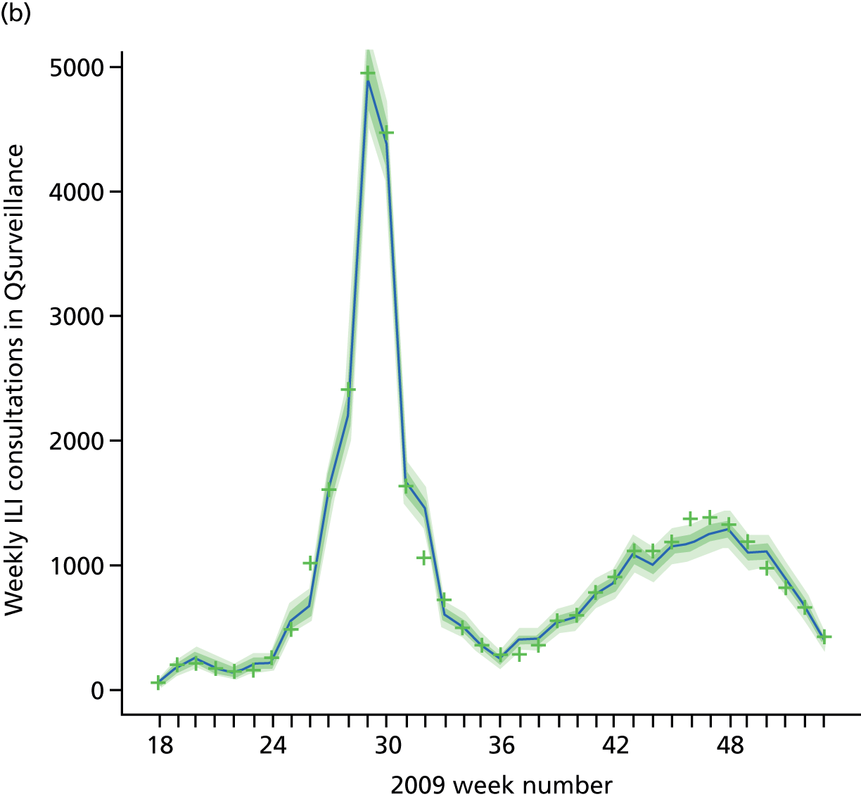
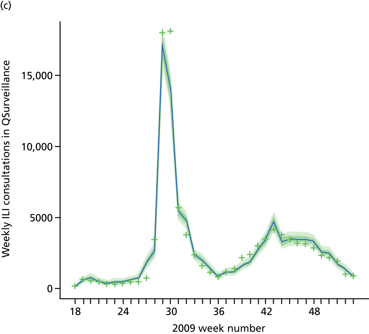

FIGURE 9.
Goodness-of-fit plot of the PR model to the serological data, stratified by age and region. Data points are marked by the dots, with the light green dots being those that are omitted by the model predicted 95% CrIs given by the vertical dashed lines. (a) Seropositivity, London, < 1 year; (b) seropositivity, London, 1–4 years; (c) seropositivity, London, 5–14 years; (d) seropositivity, London, 15–24 years; (e) seropositivity, London, 25–44 years; (f) seropositivity, London, 45–64 years; (g) seropositivity, London, ≥ 65 years; (h) seropositivity, West Midlands, < 1 year; (i) seropositivity, West Midlands, 1–4 years; (j) seropositivity, West Midlands, 5–14 years; (k) seropositivity, West Midlands, 15–24 years; (l) seropositivity, West Midlands, 25–44 years; (m) seropositivity, West Midlands, 45–64 years; (n) seropositivity, West Midlands, ≥ 65 years; (o) seropositivity, North, < 1 year; (p) seropositivity, North, 1–4 years; (q) seropositivity, North, 5–14 years; (r) seropositivity, North, 15–24 years; (s) seropositivity, North, 25–44 years; (t) seropositivity, North, 45–64 years; (u) seropositivity, North, ≥ 65 years; (v) seropositivity, South, < 1 year; (w) seropositivity, South, 1–4 years; (x) seropositivity, South, 5–14 years; (y) seropositivity, South, 15–24 years; (z) seropositivity, South, 25–44 years; (aa) seropositivity, South, 45–64 years; and (bb) seropositivity, South, ≥ 65 years. Adapted from Birrell et al. 28 © 2016, Macmillan Publishers Limited. This work is licensed under a Creative Commons Attribution 4.0 International License. The images or other third party material in this article are included in the article’s Creative Commons license, unless indicated otherwise in the credit line; if the material is not included under the Creative Commons license, users will need to obtain permission from the license holder to reproduce the material. To view a copy of this license, visit http://creativecommons.org/licenses/by/4.0/.


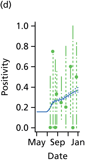
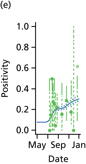

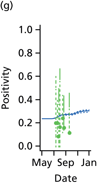
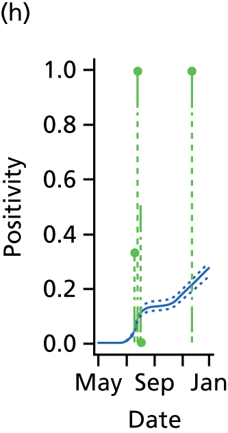


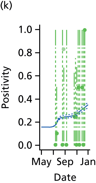
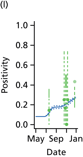
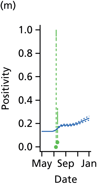

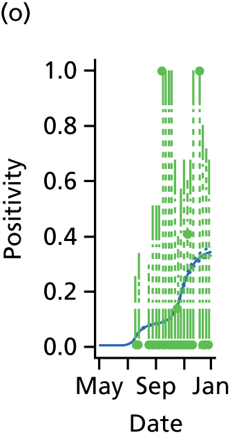
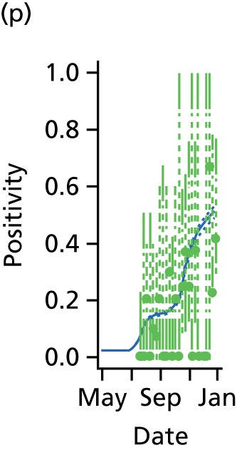
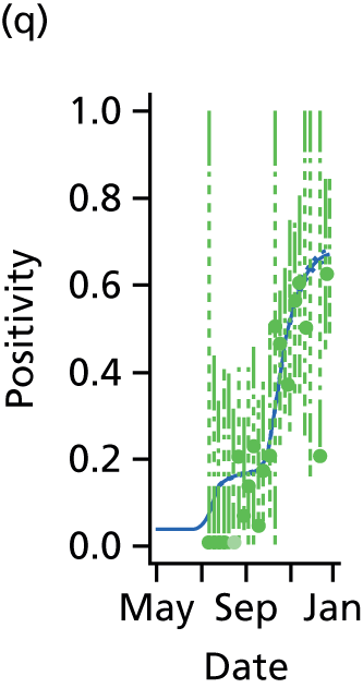

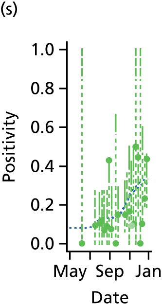
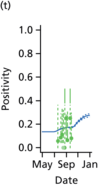
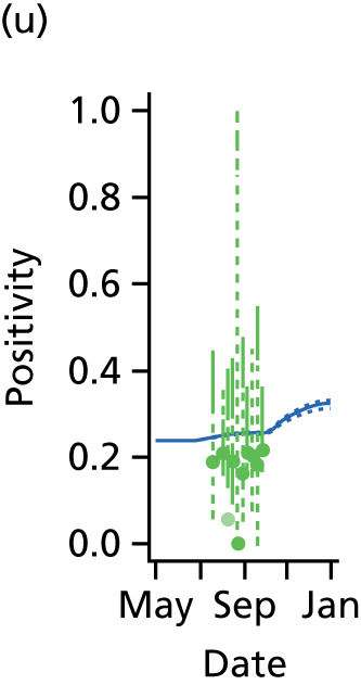

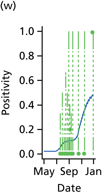

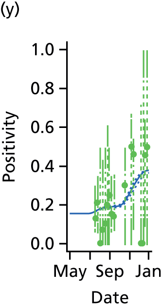


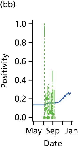
FIGURE 10.
Goodness-of-fit plot of the PR model to the weekly aggregated viropositivity data, stratified by age in London. Data points are given by the dots of variable width and colour. The width indicates the size of the denominator relative to other points in the sample plot. The colour of the points indicates the overall size of the denominator, with dark blue points being those of largest sample size. The black vertical lines give a containing 95% CrI for the data points under the model. (a) Positivity, London, < 1 year; (b) positivity, London, 1–4 years; (c) positivity, London, 5–14 years; (d) positivity, London, 15–24 years; (e) positivity, London, 25–44 years; (f) positivity, London, 45–64 years; and (g) positivity, London, ≥ 65 years. Adapted from Birrell et al. 28 © 2016, Macmillan Publishers Limited. This work is licensed under a Creative Commons Attribution 4.0 International License. The images or other third party material in this article are included in the article’s Creative Commons license, unless indicated otherwise in the credit line; if the material is not included under the Creative Commons license, users will need to obtain permission from the license holder to reproduce the material. To view a copy of this license, visit http://creativecommons.org/licenses/by/4.0/.
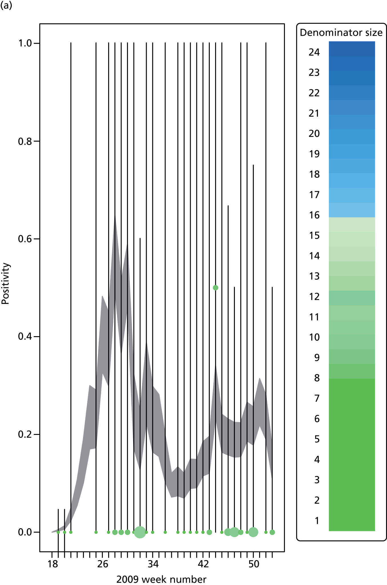
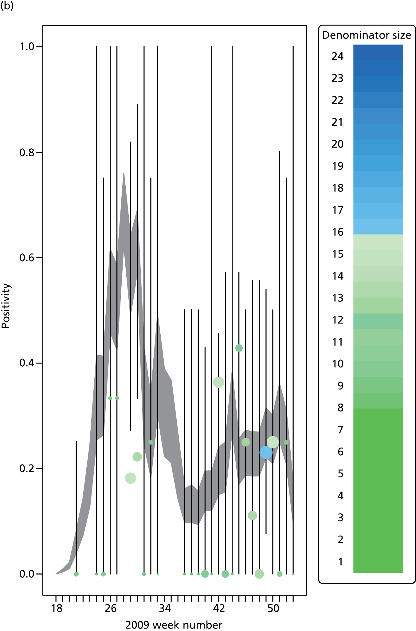


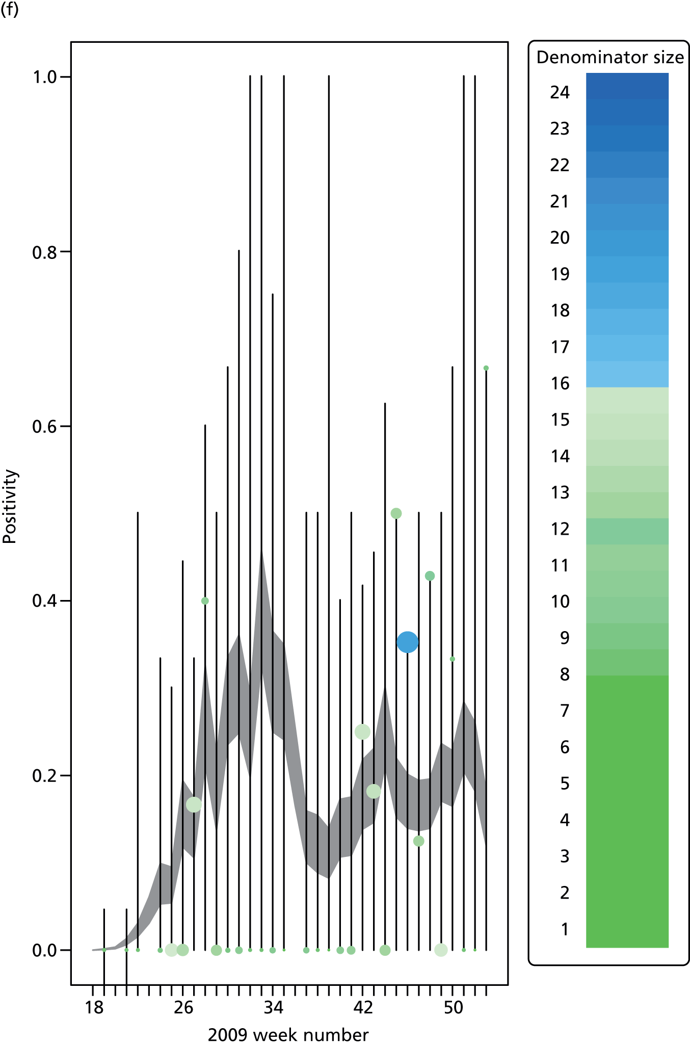

FIGURE 11.
Goodness-of-fit plot of the PR model to the weekly aggregated viropositivity data, stratified by age in the West Midlands. See figure 10 for greater detail. 28 (a) Positivity, West Midlands, < 1 year; (b) positivity, West Midlands, 1–4 years; (c) positivity, West Midlands, 5–14 years; (d) positivity, West Midlands, 15–24 years; (e) positivity, West Midlands, 25–44 years; (f) positivity, West Midlands, 45–64 years; and (g) positivity, West Midlands, ≥ 65 years. Adapted from Birrell et al. 28 © 2016, Macmillan Publishers Limited. This work is licensed under a Creative Commons Attribution 4.0 International License. The images or other third party material in this article are included in the article’s Creative Commons license, unless indicated otherwise in the credit line; if the material is not included under the Creative Commons license, users will need to obtain permission from the license holder to reproduce the material. To view a copy of this license, visit http://creativecommons.org/licenses/by/4.0/.


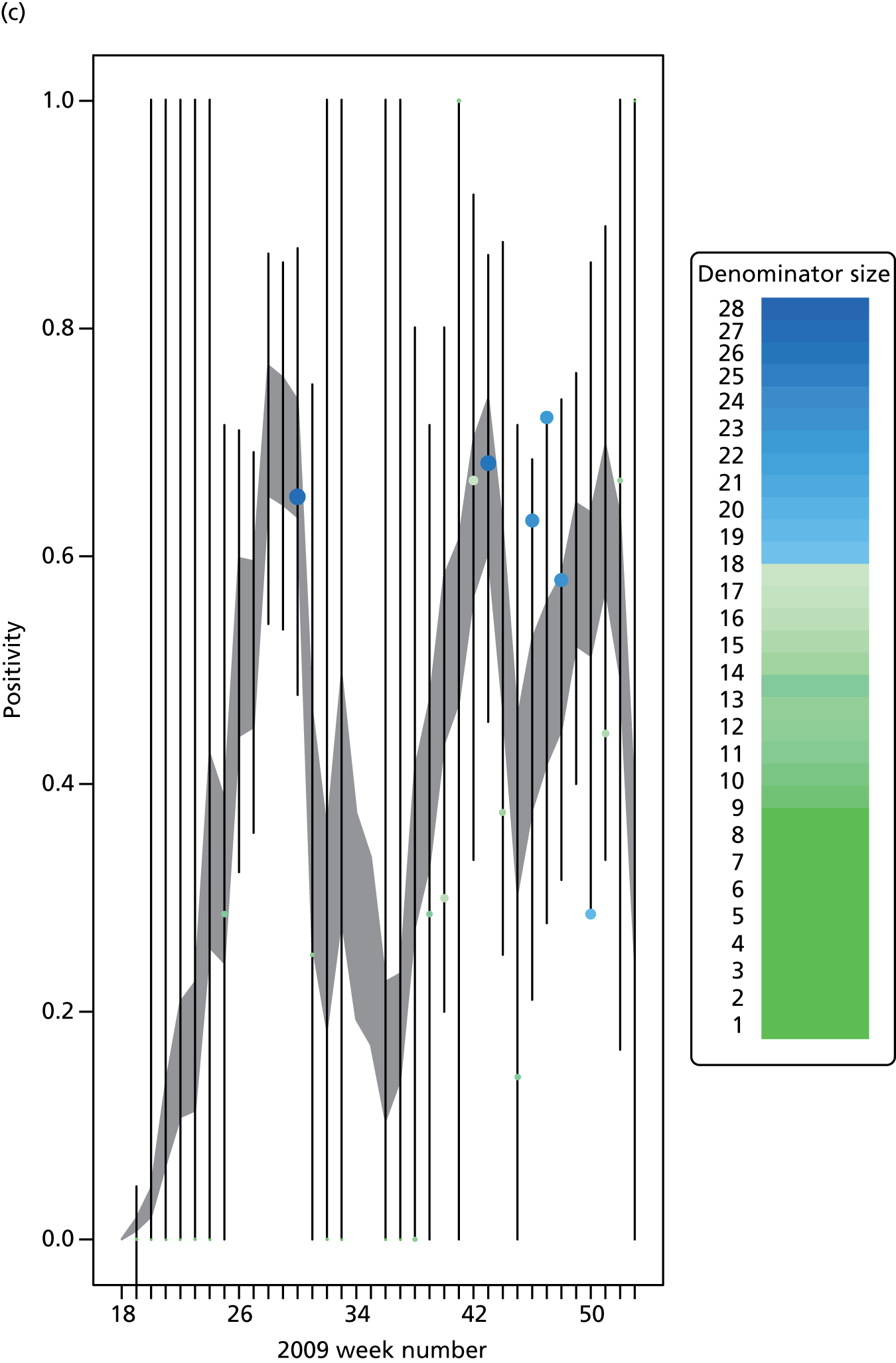


FIGURE 12.
Goodness-of-fit plot of the PR model to the weekly aggregated viropositivity data, stratified by age, in the South. See figure 10 for greater details. 28 (a) Positivity, South, < 1 year; (b) positivity, South, 1–4 years; (c) positivity, South, 5–14 years; (d) positivity, South, 15–24 years; (e) positivity, South, 25–44 years; (f) positivity, South, 45–64 years; and (g) positivity, South, ≥ 65 years. Adapted from Birrell et al. 28 © 2016, Macmillan Publishers Limited. This work is licensed under a Creative Commons Attribution 4.0 International License. The images or other third party material in this article are included in the article’s Creative Commons license, unless indicated otherwise in the credit line; if the material is not included under the Creative Commons license, users will need to obtain permission from the license holder to reproduce the material. To view a copy of this license, visit http://creativecommons.org/licenses/by/4.0/.
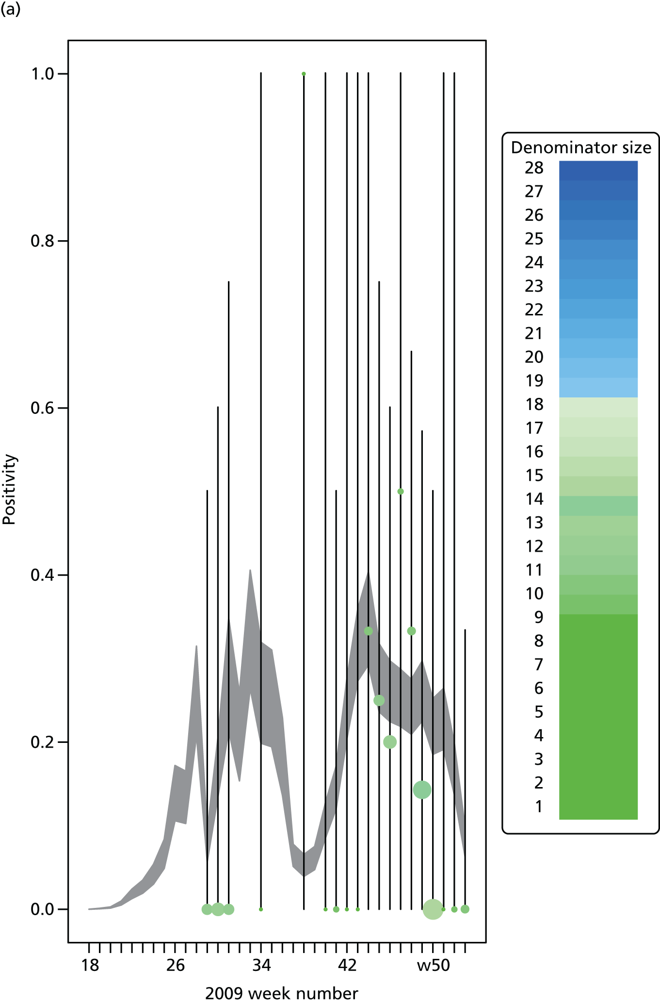
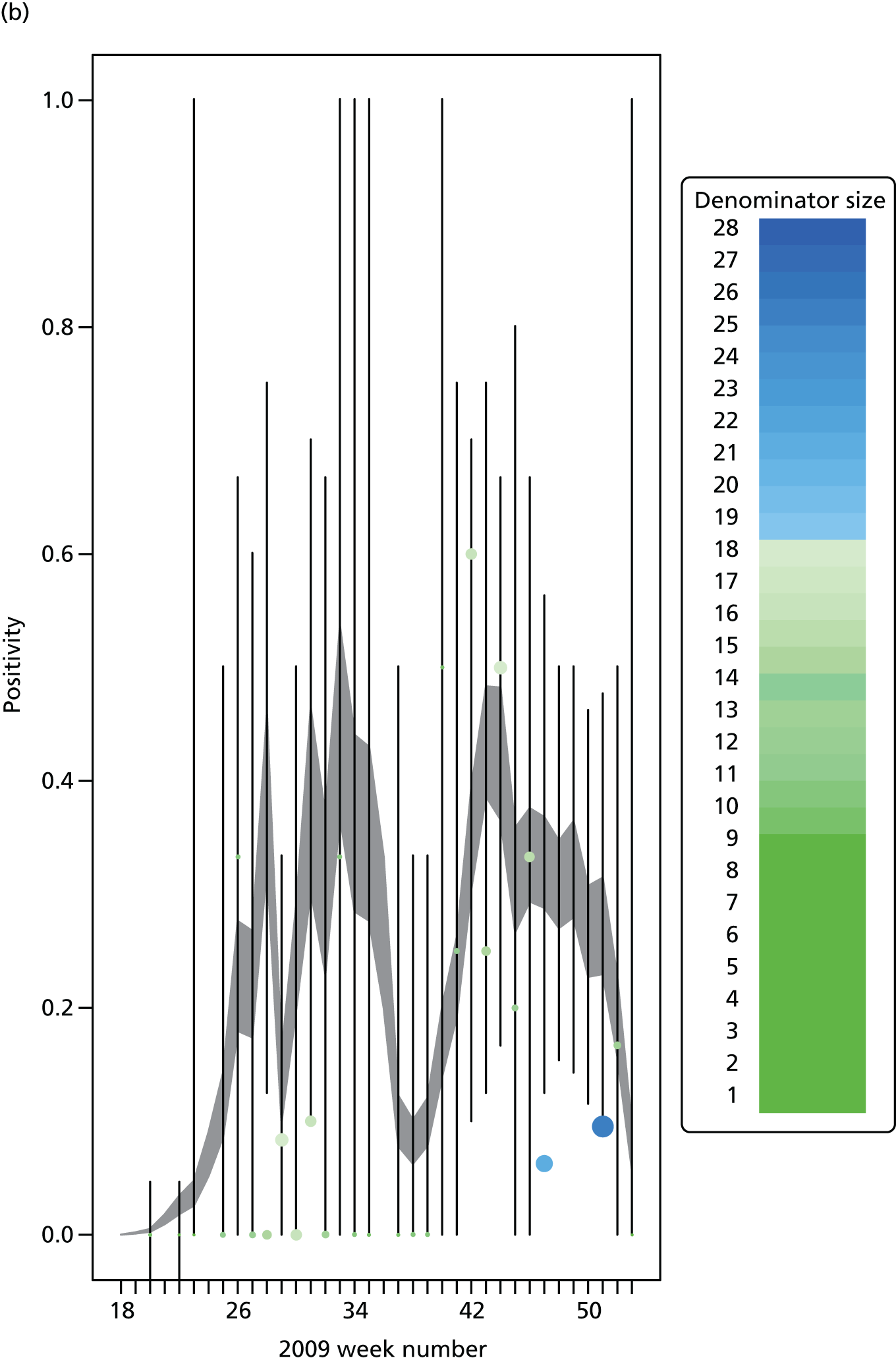
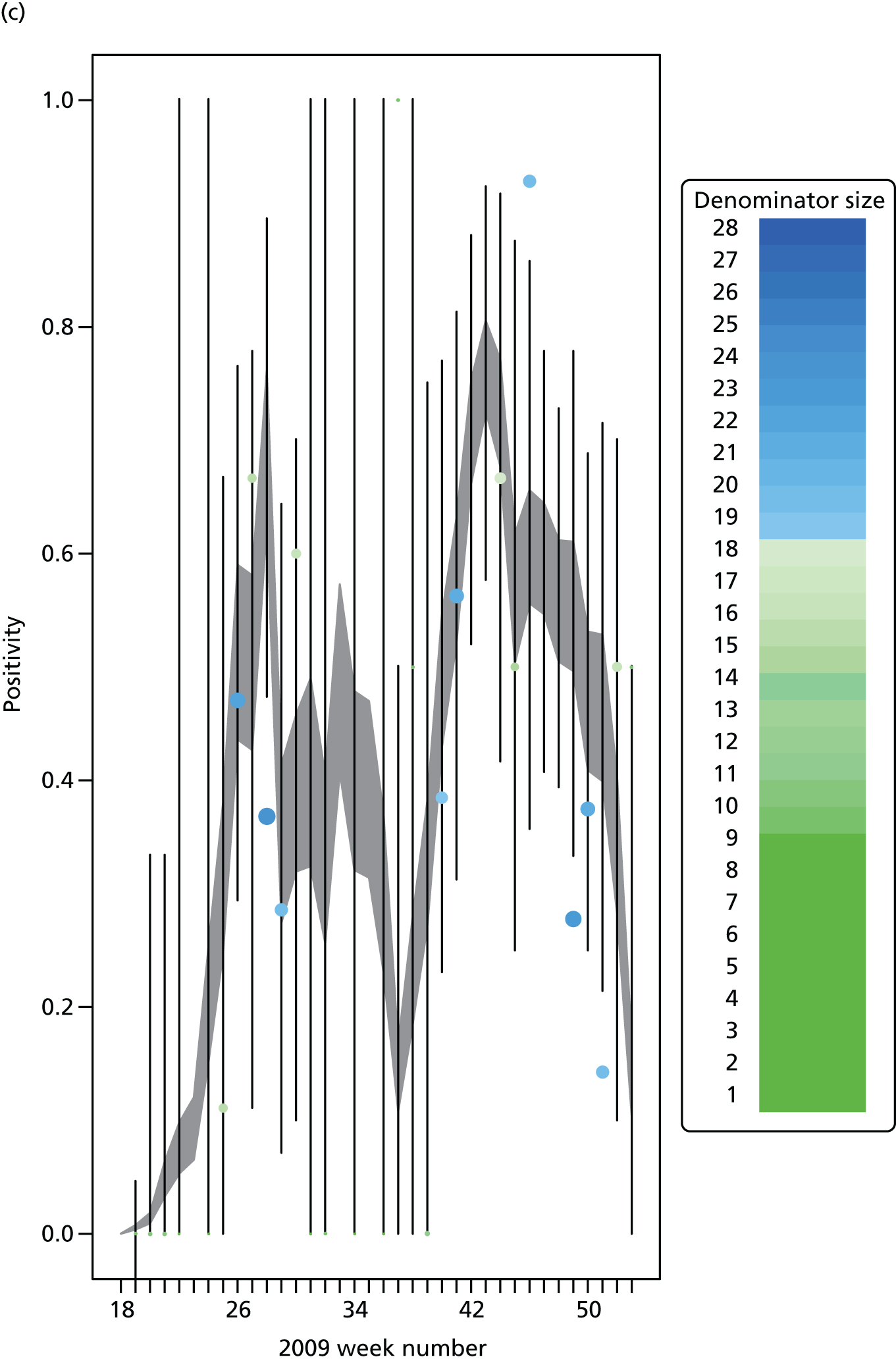

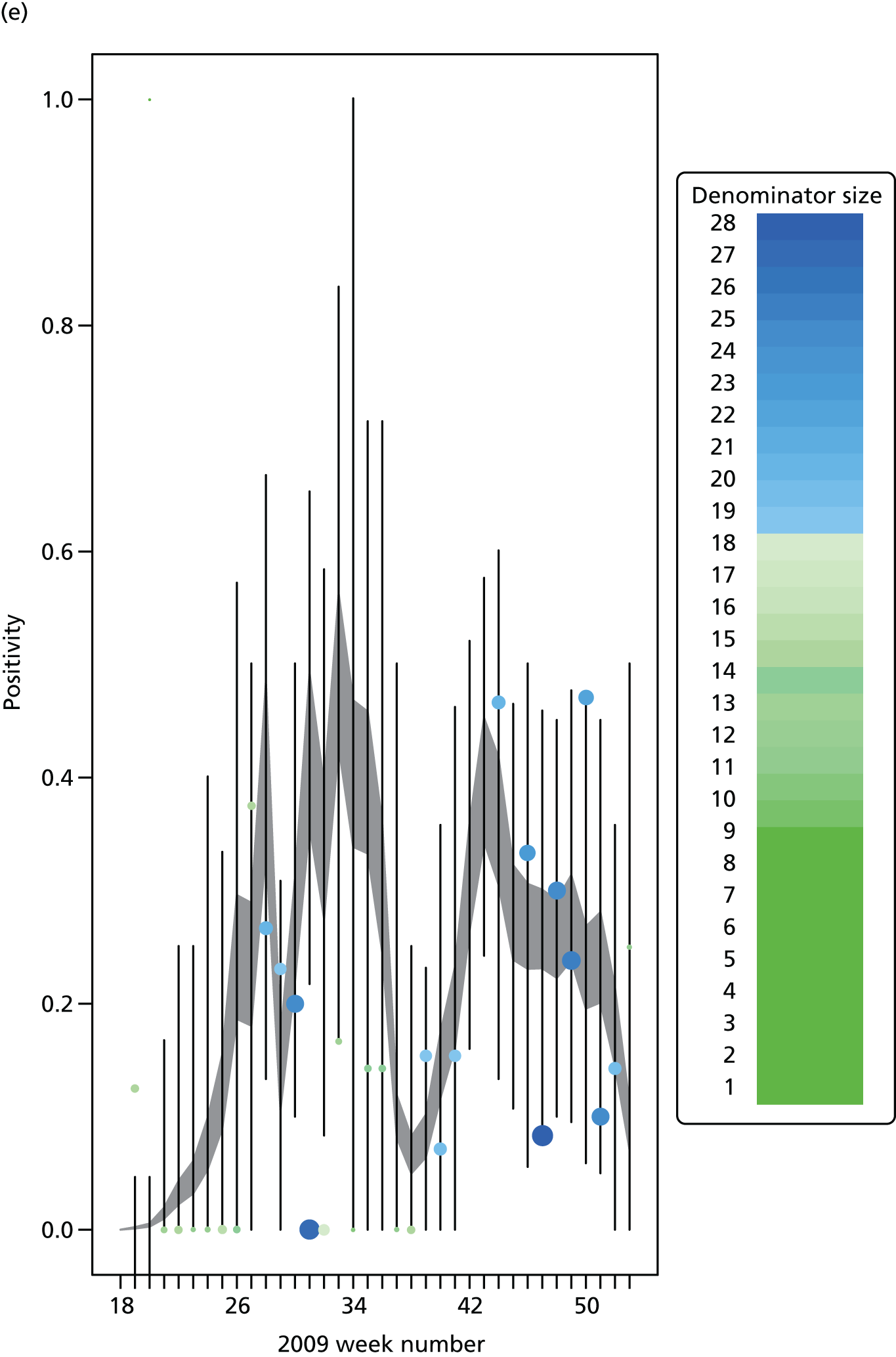
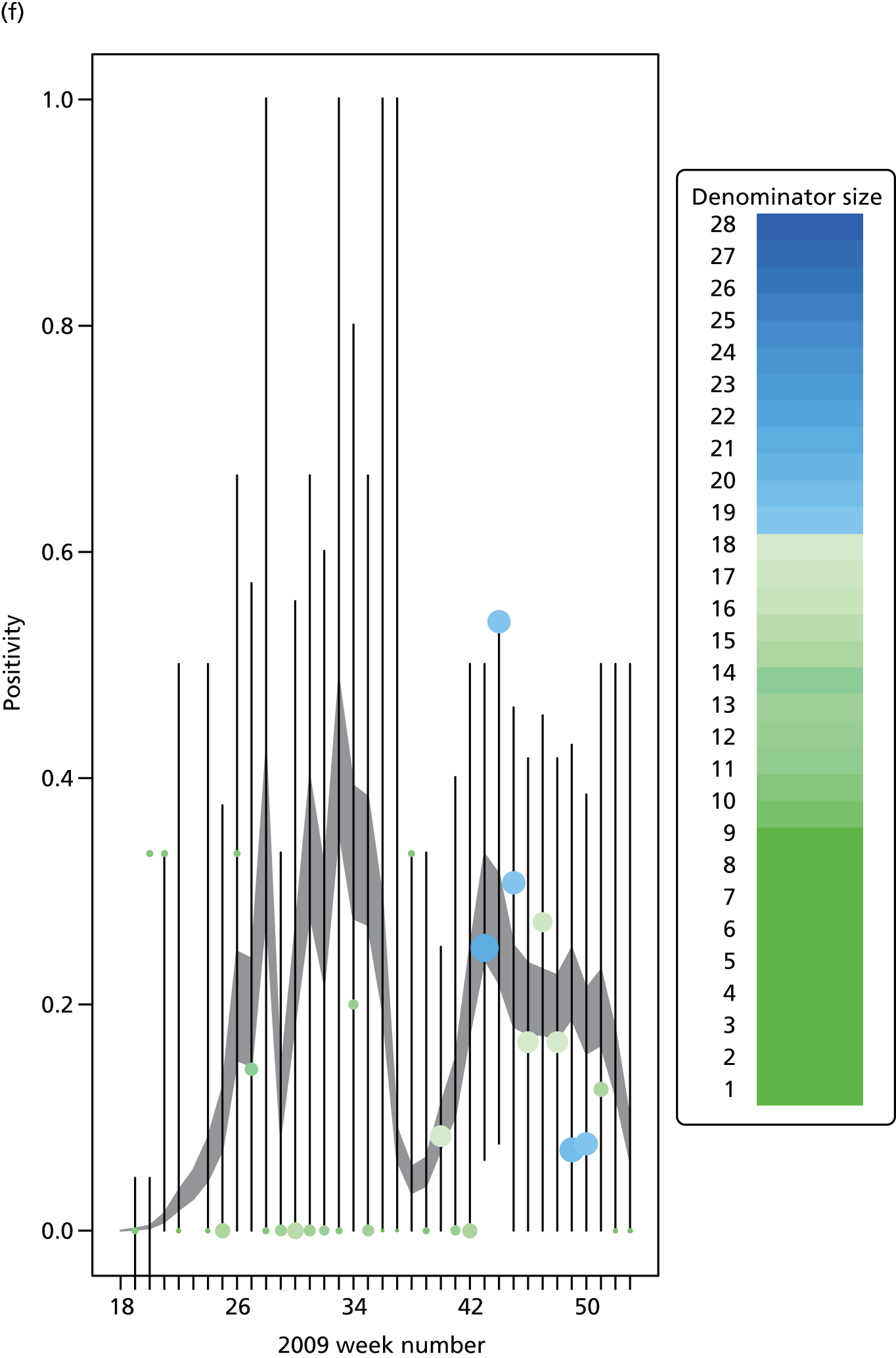

Appendix 5 Goodness-of-fit plots for the meta-region model
Presented here are plots of the goodness of fit of the best-fitting MR model to the GP consultation data, the serological data and the virological data (in all regions except the North, where denominators were frequently too small to get a reasonable comparison).
FIGURE 13.
Goodness-of-fit plot of the MR model to the GP consultation data, aggregated by age. + symbols indicate the observed number of consultations. The darker shaded areas represent the 95% CrI for the expected number of consultations, and the wider, lighter green interval gives a posterior predictive 95% CrI for the observed data, that is, 95% of the data points should lie within this wider interval. (a) Goodness of fit: total GP consultations, London; (b) Goodness of fit: total GP consultations, West Midlands; (c) Goodness of fit: total GP consultations, North; and (d) Goodness of fit: total GP consultations, South. Adapted from Birrell et al. 28 © 2016, Macmillan Publishers Limited. This work is licensed under a Creative Commons Attribution 4.0 International License. The images or other third party material in this article are included in the article’s Creative Commons license, unless indicated otherwise in the credit line; if the material is not included under the Creative Commons license, users will need to obtain permission from the license holder to reproduce the material. To view a copy of this license, visit http://creativecommons.org/licenses/by/4.0/.
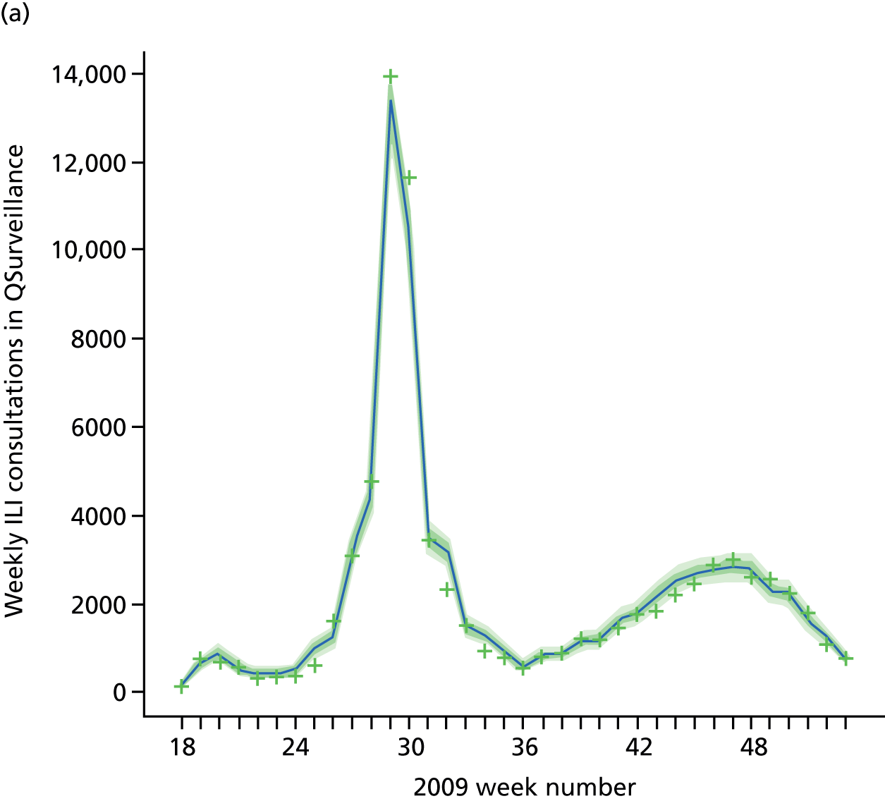

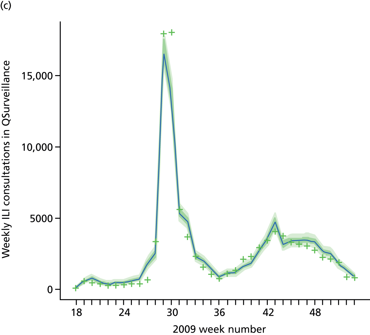

FIGURE 14.
Goodness-of-fit plot of the MR model to the serological data, stratified by age and region. Data points are marked by dots, with the light green dots being those that are omitted by the model predicted 95% CrIs shown by the vertical dashed lines. (a) Seropositivity, London, < 1 year; (b) seropositivity, London, 1–4 years; (c) seropositivity, London, 5–14 years; (d) seropositivity, London, 15–24 years; (e) seropositivity, London, 25–44 years; (f) seropositivity, London, 45–64 years; (g) seropositivity, London, ≥ 65 years; (h) seropositivity, West Midlands, < 1 year; (i) seropositivity, West Midlands, 1–4 years; (j) seropositivity, West Midlands, 5–14 years; (k) seropositivity, West Midlands, 15–24 years; (l) seropositivity, West Midlands, 25–44 years; (m) seropositivity, West Midlands, 45–64 years; (n) seropositivity, West Midlands, ≥ 65 years; (o) seropositivity, North, < 1 year; (p) seropositivity, North, 1–4 years; (q) seropositivity, North, 5–14 years; (r) seropositivity, North, 15–24 years; (s) seropositivity, North, 25–44 years; t) seropositivity, North, 45–64 years; (u) seropositivity, North, ≥ 65 years; (v) seropositivity, South, < 1 year; (w) seropositivity, South, 1–4 years; (x) seropositivity, South, 5–14 years; (y) seropositivity, South, 15–24 years; (z) seropositivity, South, 25–44 years; (aa) seropositivity, South, 45–64 years; and (bb) seropositivity, South, ≥ 65 years. Adapted from Birrell et al. 28 © 2016, Macmillan Publishers Limited. This work is licensed under a Creative Commons Attribution 4.0 International License. The images or other third party material in this article are included in the article’s Creative Commons license, unless indicated otherwise in the credit line; if the material is not included under the Creative Commons license, users will need to obtain permission from the license holder to reproduce the material. To view a copy of this license, visit http://creativecommons.org/licenses/by/4.0/.

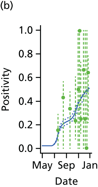


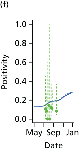

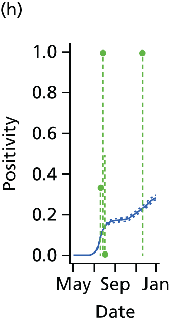
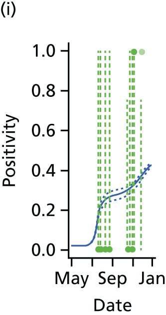
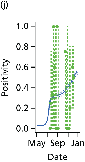


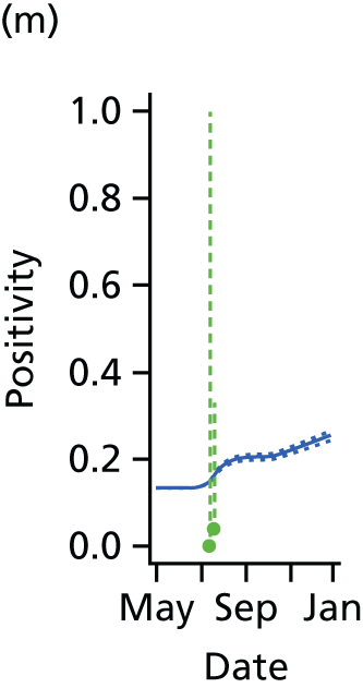
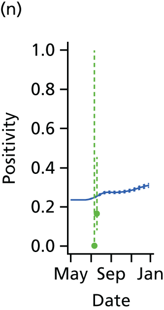
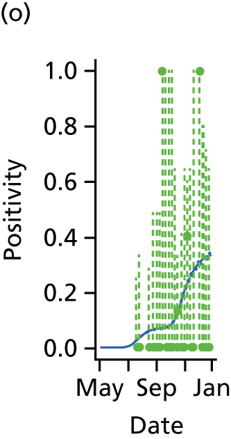
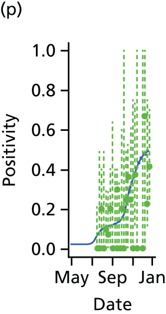


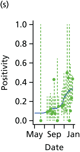
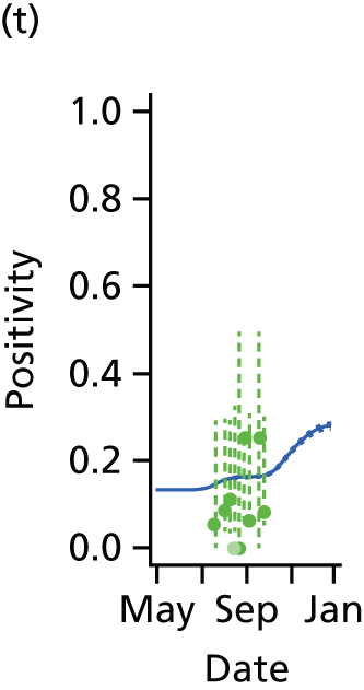


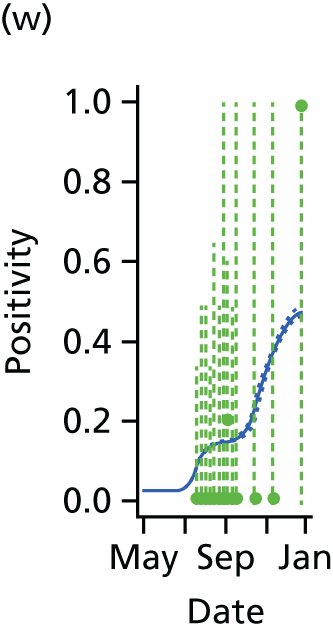
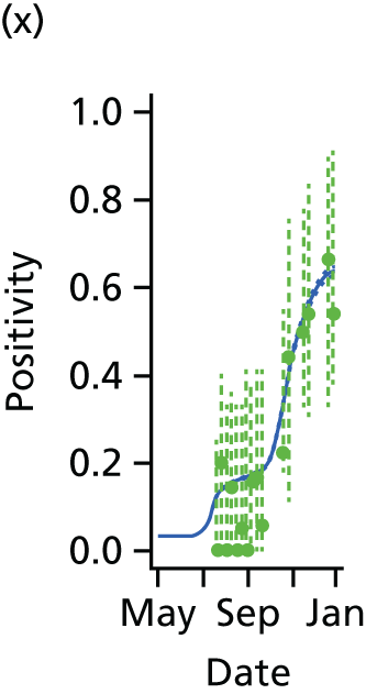


FIGURE 15.
Goodness-of-fit plot of the MR model to the weekly aggregated viropositivity data, stratified by age in London. Data points are given by the dots of variable width and colour. The width indicates the size of the denominator relative to other points in the same plot. The colour of the points indicates the overall size of the denominator, with dark blue points being those of largest sample size. The black vertical lines give a containing 95% CrI for the data points under the model. (a) Positivity, London, < 1 year; (b) positivity, London, 1–4 years; (c) positivity, London, 5–14 years; (d) positivity, London, 15–24 years; (e) positivity, London, 25–44 years; (f) positivity, London, 45–64 years; and (g) positivity, London, ≥ 65 years. Adapted from Birrell et al. 28 © 2016, Macmillan Publishers Limited. This work is licensed under a Creative Commons Attribution 4.0 International License. The images or other third party material in this article are included in the article’s Creative Commons license, unless indicated otherwise in the credit line; if the material is not included under the Creative Commons license, users will need to obtain permission from the license holder to reproduce the material. To view a copy of this license, visit http://creativecommons.org/licenses/by/4.0/.


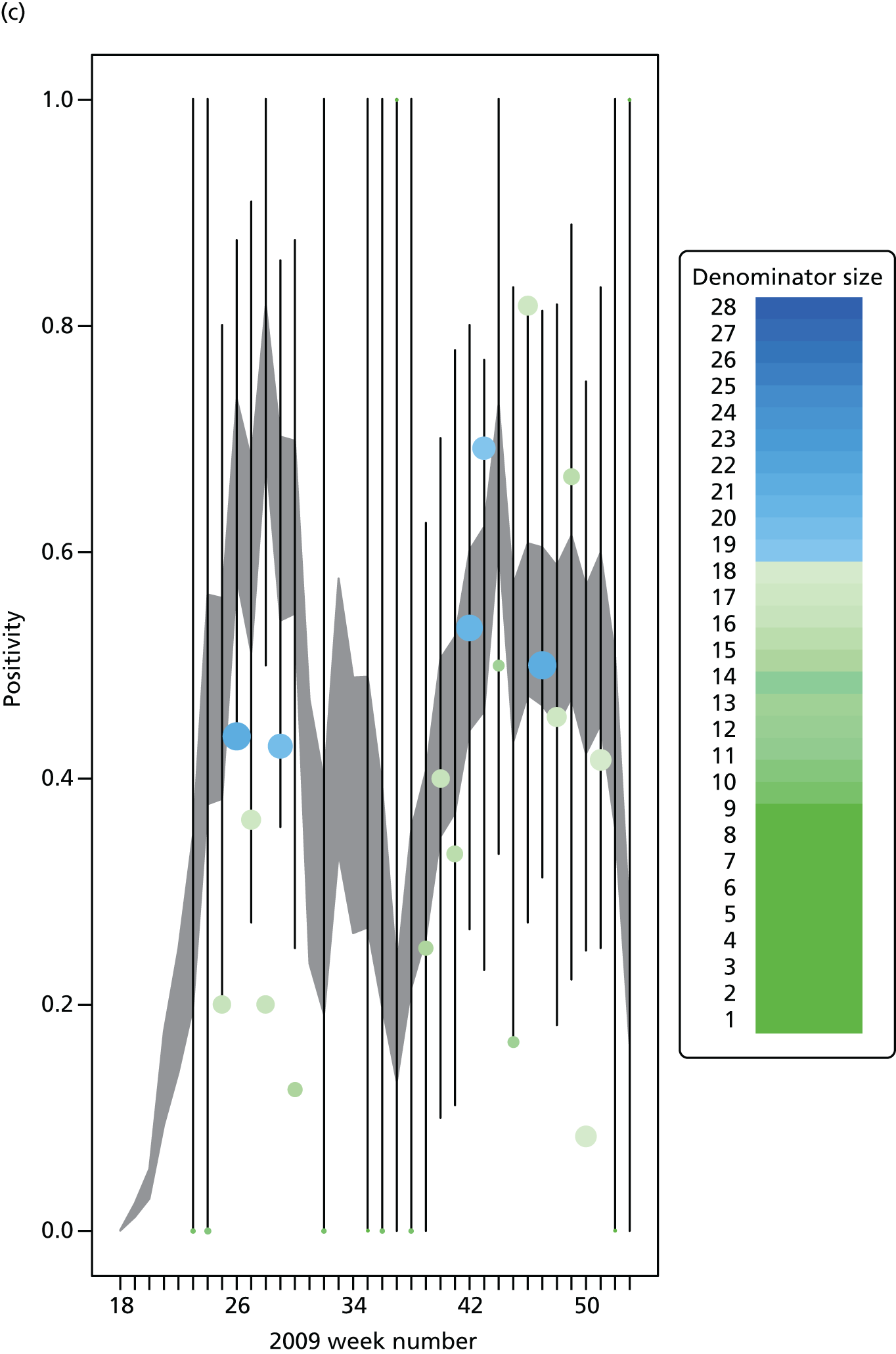


FIGURE 16.
Goodness-of-fit plot of the MR model to the weekly aggregated viropositivity data, stratified by age, in the West Midlands. See figure D3 for greater detail. (a) Positivity, West Midlands, < 1 year; (b) positivity, West Midlands, 1–4 years; (c) positivity, West Midlands, 5–14 years; (d) positivity, West Midlands, 15–24 years; (e) positivity, West Midlands, 25–44 years; (f) positivity, West Midlands, 45–64 years; and (g) positivity, West Midlands, ≥ 65 years. Adapted from Birelli et al. 28 © 2016, Macmillan Publishers Limited. This work is licensed under a Creative Commons Attribution 4.0 International License. The images or other third party material in this article are included in the article’s Creative Commons license, unless indicated otherwise in the credit line; if the material is not included under the Creative Commons license, users will need to obtain permission from the license holder to reproduce the material. To view a copy of this license, visit http://creativecommons.org/licenses/by/4.0/.

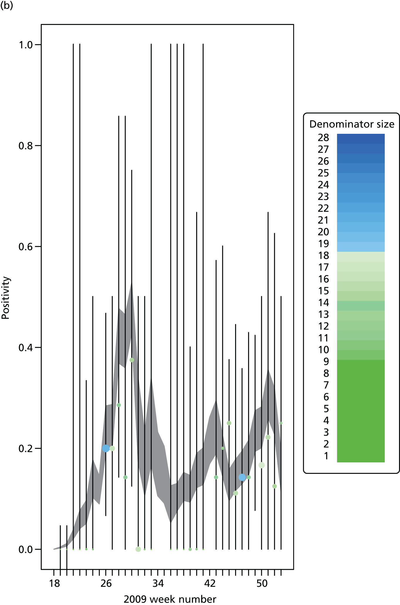

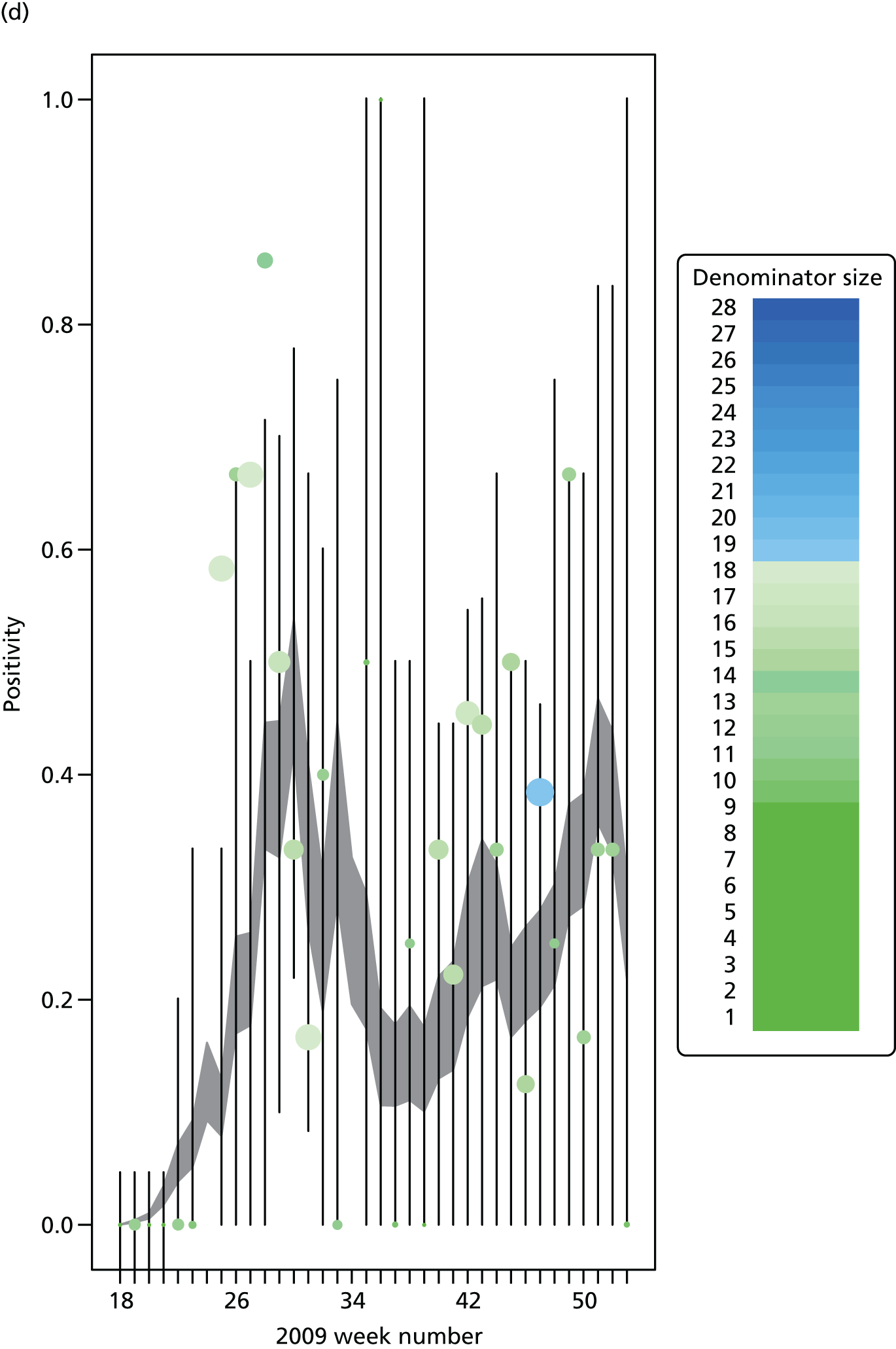
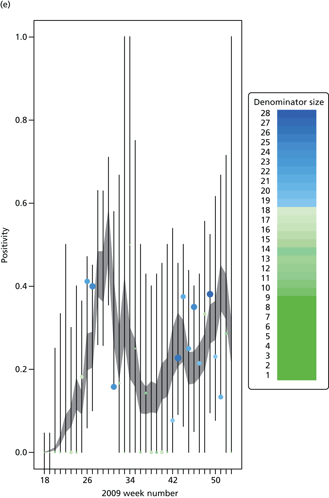
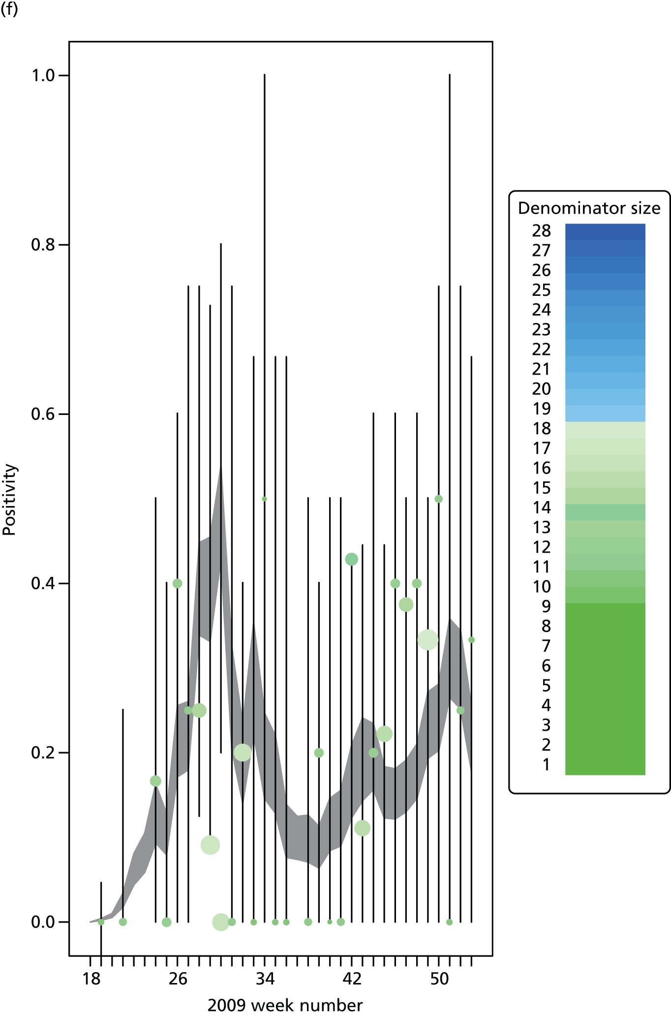
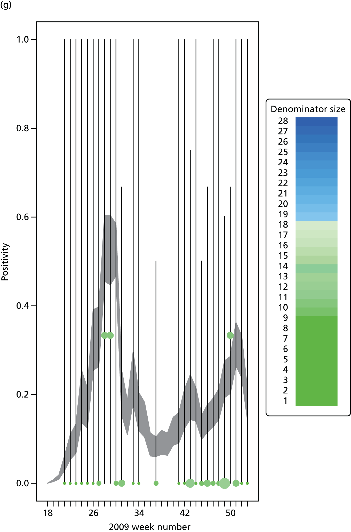
FIGURE 17.
Goodness-of-fit plot of the MR model to the weekly aggregated viropositivity data, stratified by age, in the South. See figure D3 for greater detail. (a) Positivity, South, < 1 year; (b) positivity, South, 1–4 years; (c) positivity, South, 5–14 years; (d) positivity, South, 15–24 years; (e) positivity, South, 25–44 years; (f) positivity, South, 45–64 years; and (g) positivity, South, ≥ 65 years. Adapted from Birelli et al. 28 © 2016, Macmillan Publishers Limited. This work is licensed under a Creative Commons Attribution 4.0 International License. The images or other third party material in this article are included in the article’s Creative Commons license, unless indicated otherwise in the credit line; if the material is not included under the Creative Commons license, users will need to obtain permission from the license holder to reproduce the material. To view a copy of this license, visit http://creativecommons.org/licenses/by/4.0/.


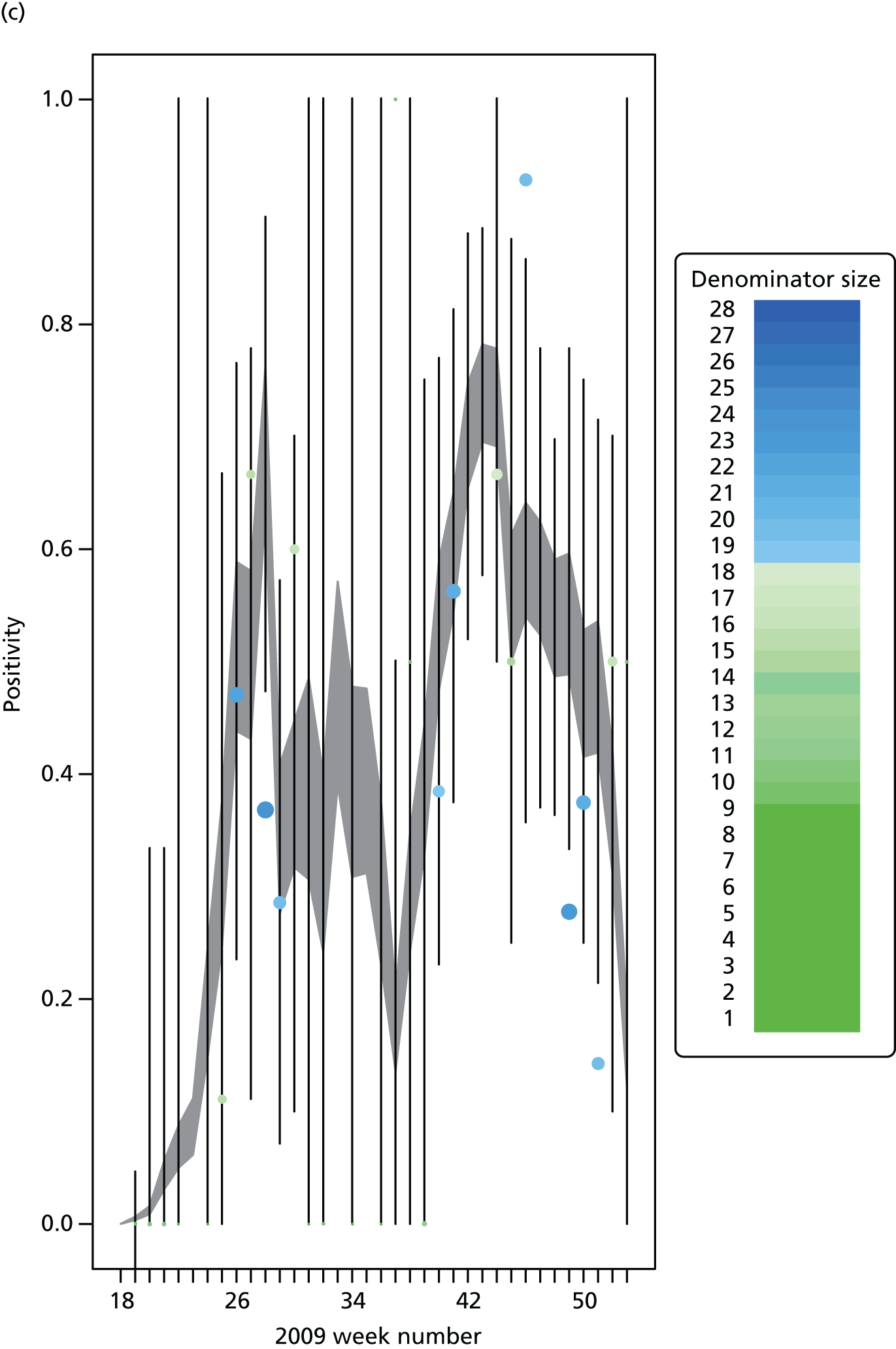


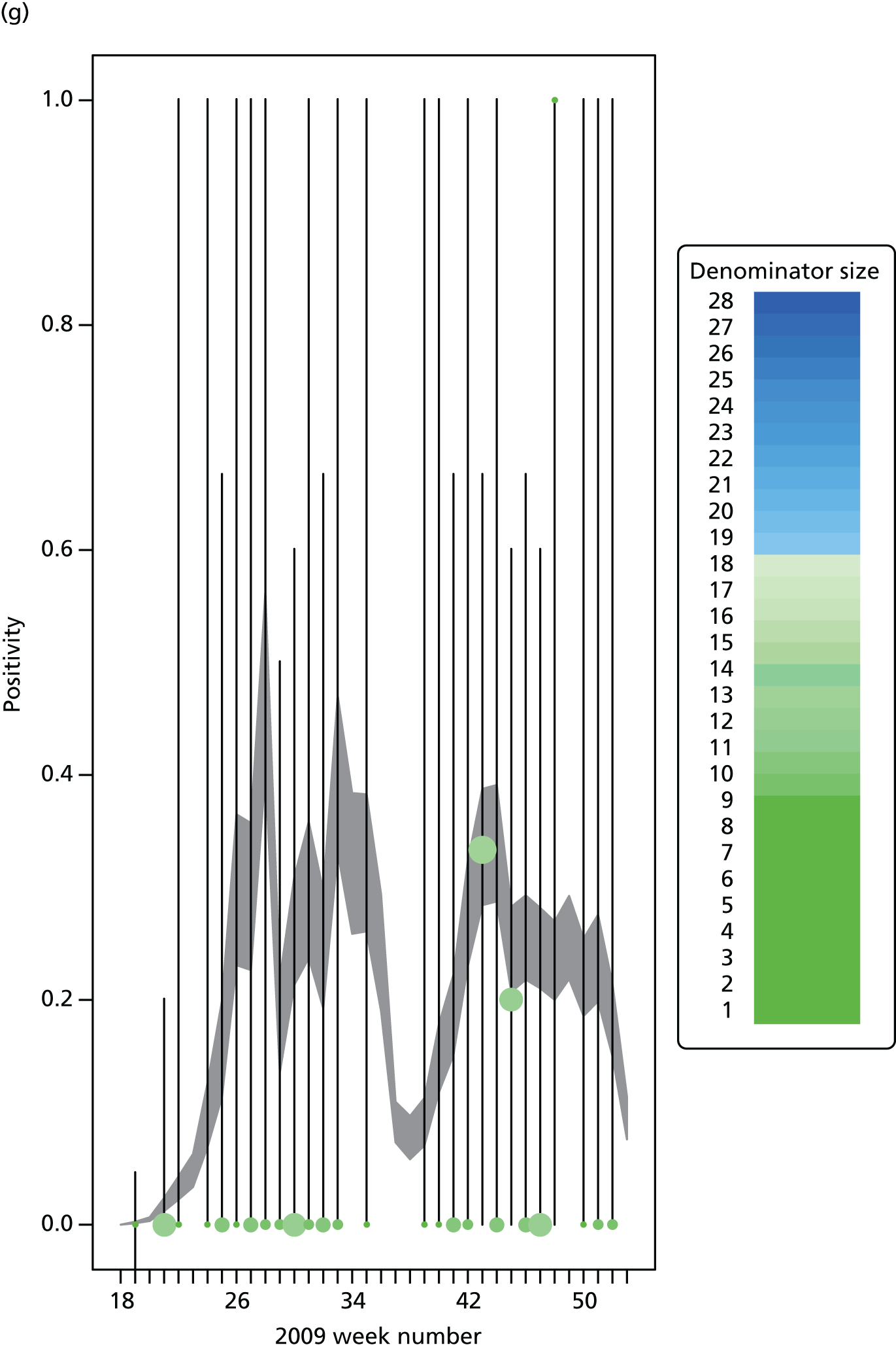
Glossary
- R0
- The reproductive number, a key epidemic characteristic defined as the average number of secondary infections caused by a single infection within a fully susceptible population.
List of abbreviations
- CrI
- credible interval
- ESS
- effective sample size
- GOR
- Government Office Region
- GP
- general practice
- HPA
- Health Protection Agency
- ICC
- intraclass correlation coefficient
- ICU
- intensive care unit
- ILI
- influenza-like illness
- KL
- Küllback–Leibler
- MCMC
- Markov chain Monte Carlo
- MH
- Metropolis–Hastings
- MR
- meta-region
- NHS
- National Healthcare Service
- NPFS
- National Pandemic Flu Service
- ONS
- Office for National Statistics
- PCR
- polymerase chain reaction
- PHE
- Public Health England
- POLYMOD
- Improving Public Health Policy in Europe through the Modelling and Economic Evaluation of Interventions for the Control of Infectious Diseases
- PR
- parallel region
- RCGP
- Royal College of General Practitioners
- RMN
- Regional Microbiology Network
- SEIR
- susceptible, exposed, infectious, recovered
- SHA
- Strategic Health Authority
- SMC
- sequential Monte Carlo
- USISS
- UK Severe Influenza Surveillance System