Notes
Article history
The research reported in this issue of the journal was funded by the PHR programme as project number 11/3005/13. The contractual start date was in April 2013. The final report began editorial review in January 2017 and was accepted for publication in June 2017. The authors have been wholly responsible for all data collection, analysis and interpretation, and for writing up their work. The PHR editors and production house have tried to ensure the accuracy of the authors’ report and would like to thank the reviewers for their constructive comments on the final report document. However, they do not accept liability for damages or losses arising from material published in this report.
Declared competing interests of authors
Melissa C Lott reports grants from BHP Billiton outside the submitted work. Mike Holland reports personal fees from the NHS during the conduct of the study.
Permissions
Copyright statement
© Queen’s Printer and Controller of HMSO 2018. This work was produced by Williams et al. under the terms of a commissioning contract issued by the Secretary of State for Health and Social Care. This issue may be freely reproduced for the purposes of private research and study and extracts (or indeed, the full report) may be included in professional journals provided that suitable acknowledgement is made and the reproduction is not associated with any form of advertising. Applications for commercial reproduction should be addressed to: NIHR Journals Library, National Institute for Health Research, Evaluation, Trials and Studies Coordinating Centre, Alpha House, University of Southampton Science Park, Southampton SO16 7NS, UK.
2018 Queen’s Printer and Controller of HMSO
Chapter 1 Introduction
Climate change is one of the most significant environmental issues facing humanity at the present time. There are major concerns over the increase in global temperatures and the concomitant impacts on weather, extreme events and the spread of disease. Most research on the impact of climate change has concentrated on the effects of a changing climate. The UK’s Health Protection Agency (now Public Health England) has assessed the potential impact of a changing climate on health in the UK and identified effects on air pollution, aeroallergens, the indoor environment, ultraviolet radiation, flooding, vector-borne diseases, and water- and food-borne diseases. 1
However, measures to mitigate climate change will involve the reduction of emissions of carbon dioxide (CO2) and other greenhouse gases and most of these measures will, at the same time, reduce air pollution, resulting in cobenefits to health and the wider environment. A policy document from the Department for Environment Food & Rural Affairs (Defra) pointed out the potential benefits of aligning climate and air pollution policies. 2 Initial assessments tended to concentrate on the effects of a changing climate, but more recently emission changes have also been considered. However, although there are significant possible cobenefits for air quality and public health from ambitious climate policies, there can also be antagonisms. Some measures that are potentially good for climate can have detrimental effects on air quality and hence public health. Burning wood, for example, is to an extent carbon neutral, but can emit larger amounts of particulate matter (PM) than other fuel sources it replaces, such as gas. The cobenefits and trade-offs have more recently been discussed3 and are explored quantitatively in this report.
Many studies have concentrated on the impact of climate change and climate policies on ozone (O3) concentrations. Most studies cover regional scales and as such use models with relatively coarse spatial scales. In a recent study in Europe, Hendricks et al. 4 used the LOTOS-EUROS model with a grid resolution of 0.5° × 0.25° (approximately 50 × 25 km), and energy scenarios from the price-induced market equilibrium system model and the greenhouse gas–air pollution interaction and synergies (GAINS) integrated assessment model used by the European Commission. The energy scenarios were a ‘current legislation’ case and an ambitious decarbonisation scenario reducing greenhouse gas emissions by 80% by 2050. The authors concluded that health damage from O3 would decline significantly in both scenarios under current climate conditions, but the possible increase in O3 concentrations as a result of a warming climate might offset this improvement. As discussed below in relation to our results (see Chapter 6, Air quality: ozone), it is possible that the large grid size in the model used in this work may have missed the fine-scale increase in urban O3 resulting from a decrease in urban oxides of nitrogen (NOx) emissions.
A paper by Watson et al. 5 used an ensemble approach with four chemical transport models using a horizontal grid resolution of 50 km. This updated an earlier study using only the CHIMERE model,6 also using the same grid resolution, which showed that emission changes were potentially more important than changing temperatures or intercontinental transport of pollutants. The study by Watson et al. 5 used greenhouse gas emissions from the Intergovernmental Panel on Climate Change Representative Concentration Pathways 4.5 scenario, but air pollutant emissions from the Evaluating the Climate and Air Quality Impacts of Short-Lived Pollutants (ECLIPSE) project scenario v4a (URL: http://eclipse.nilu.no; accessed 6 February 2018). They concluded that reductions in average O3 of 4–5 parts per billion (p.p.b.) could be attained across Europe in the current legislation scenario, with a further 3 p.p.b. from implementing maximum technologically feasible measures. In a more aggressive climate mitigation scenario, the authors found an increase in wintertime O3 associated with large reductions in NOx emissions and reasoned that this would be of less concern to health because of the lack of evidence for adverse effects from wintertime O3.
Studies of the links between climate change and air pollution have been carried out beyond Europe. Using the integrated model to assess the global environment (IMAGE) on a global scale, Braspenning Radu et al. 7 modelled long-term global and regional scenarios to explore synergies between climate and air quality policies. They found that in Asia, and other developing regions, a combination of climate and air pollution policies was needed to bring air pollution levels to the levels of today. Other studies outside Europe include studies on O3 in China,8,9 pollutants in the USA,10,11 a global study on O3 and particulate matter of ≤ 2.5 µm (PM2.5),12 and a study on the warming effect of removing aerosol in the USA for air pollution reasons. 13 The last study addresses one of the antagonistic effects on climate of reducing air pollution – the so-called ‘secondary’ aerosol components of PM2.5 and particulate matter of ≤ 10 µm (PM10) – made up primarily of ammonium sulphate and ammonium nitrate, which act to reflect incoming solar radiation and hence offer protection against climate warming. An antagonism in the opposite sense is afforded by the increased use of biomass (wood) burning, which, although low in carbon emissions, can emit PM, resulting in additional health impact. A recent review of the impact of biomass burning on air quality in Europe14 found that biomass burning can contribute 2.7–11.6% of average PM10 concentrations in winter at current levels. This is of concern given the strong evidence linking PM10 concentrations with mortality and morbidity, but the possible increase in biomass burning, encouraged by climate policies (URL: www.ofgem.gov.uk/environmental-programmes/domestic-rhi and URL: www.ofgem.gov.uk/environmental-programmes/non-domestic-rhi; accessed 6 February 2018), is of further concern and is addressed in the current study. The increased use of biomass could have further indirect impact on air pollution and a study addressing the impact on O3 from the increase in tree growth has been published. 15
A recent study, which is similar in concept to the current project, concerns the impact of climate change and climate-related policies in Portugal. 16 The authors modelled the whole of Portugal at a spatial resolution of 9 km, the northern region at 3 km and the Porto metropolitan areas with a grid size of 1 km. They projected decreases in nitrogen dioxide (NO2), but suggested that PM10 and O3 could increase in the Porto municipality, the latter as a result of the reduced removal of O3 via the reaction with nitrogen oxide. We discuss this in the context of Great Britain (GB) below.
The influential review of the economics of climate change by Stern17 made only brief mention of the monetary cobenefits of climate policies, and did not give details or specifically mention air quality, and made no attempt to quantify the impact on air quality and on public health outcomes. A subsequent economic analysis18 concluded that the cobenefits could be on average US$49/tonne CO2.
Some earlier studies assessed the cobenefits of air quality and climate policies at a regional level in Europe, at a relatively coarse spatial scale (generally 25- to 50-km grids). Several of these studies are based on a so-called ‘integrated assessment model’ [the regional air pollution information and simulation (RAINS) model] and the extension to include greenhouse gases known as GAINS, developed at the International Institute for Applied Systems Analysis (IIASA) in Austria. These models calculate optimal cost pathways to achieve specified environmental targets. Originally developed in Europe, at that time GAINS was unable to employ spatial resolution better than 25 × 25 km grid squares. The European Environment Agency19 used the model to study the ancillary air pollution benefits in Europe of three scenarios, the most ambitious of which reduced CO2-equivalent emissions by 40% by 2030 on a 1990 base. The work concluded that in the baseline scenario there would be 311,000 premature deaths in Europe from PM2.5 and O3 exposures, but that these would reduce to 288,000 in the ambitious climate scenario. For three climate scenarios tested in the UK, compared with a baseline of 6.9 months loss of life expectancy in 2000, the ambitious climate scenario gave a loss of 2.2 months. The scenario aimed solely at air quality targets in future showed a loss of 3.4 months, but the less ambitious climate scenario showed a smaller improvement of 4.8 months.
This early work highlights the importance of optimised scenarios for public health improvements. A study by van Vuuren et al. ,20 also using the RAINS model, assessed the monetary benefits for Europe as a whole. For the policies then in place, they found the total benefits of implementing Kyoto Protocol policies to be €2.5B–7B as reduced costs of air pollution abatement. The Netherlands Environmental Assessment Agency21 performed a global assessment of the local air quality implications of meeting climate change goals in 2050. Its conclusion was that significant health benefits could arise and might be an added incentive for developing countries to pursue climate policies. These local air quality health assessments were carried out in a rudimentary manner at an even coarser level than the RAINS model.
A further study22 illustrated the trade-offs involved in reducing air pollutants such as sulphur dioxide (SO2), which act to cool the Earth’s climate. They suggested that, in formulating policies targeted at climate, reductions in the pollutants SO2 and NOx should be ignored because elevated concentrations contribute to cooling of the earth’s surface, even though reductions would bring health and environmental benefits.
A global study reporting the ancillary benefits to air pollution from improvements to the world’s motor vehicle fleets has been published. 23 This work showed that stringent emission controls, especially from diesel engines, are required to achieve improved public health. An analysis of the UK policy of encouraging the use of diesel cars on climate change/fuel economy grounds,24 estimated that the consequent increased emission of particles would be responsible for 20–300 deaths per year in the UK. A recent assessment of the benefits to both air quality and climate change over the globe has been published,25 and showed that reducing the so-called short-lived climate pollutants (black carbon, methane and O3) could have major health benefits, particularly in Asia, as well as mitigating near-term (≈40 years) climate change.
An early paper specifically addressing the implications of climate policies for the UK was published. 26 This considered the impact on air quality of what was at that time a hypothetical UK climate change target of 60% reduction in CO2 equivalents by 2050. The study showed that impact of air pollution on mortality and morbidity in London in 2050 could be roughly halved compared with the ‘business as usual’ situation in 2050. Since that paper, an even more ambitious target of 80% reduction is now embeded in UK law, as discussed below.
A series of papers in The Lancet in 2009 addressed climate change issues. Two papers27 studied the implications for health of a low-carbon vehicle fleet and another28 investigated the benefits of increased energy efficiency in the UK housing stock. None of these papers used policies based on government policies across all sectors of the economy – these have only recently emerged – nor did they assess cobenefits across the whole population of the UK.
More recently, in 2015, the Lancet Commission was set up to map out the impact of climate change and the policies which might lead to the greatest improvement in public health. The coverage is global, and a recent paper29 sets out a strategy for tracking indicators of health and climate change, including the cobenefits from air pollution. The paper also noted that tackling climate change could offer the greatest global health opportunity of the twenty-first century. The same conclusion, applied to the UK, was the inspiration for the present study.
The broad implications for air quality and public health of choices for climate policies in the UK have recently become clearer. Following the adoption of the UK’s Climate Change Act 2008 (CCA),30 the government published The UK Low Carbon Transition Plan,31 which concluded that, although some policies would result in large improvements in air quality, the adverse health effects from an unmanaged major uptake of biomass (wood) in the residential sector would outweigh the air quality/health benefits from all the changes in other sectors, at a net air quality cost rising to £2.6B in 2022. More recently, the then Department of Energy and Climate Change (DECC) published The Carbon Plan: Delivering Our Low Carbon Future,32 which set out several options for achieving the 2050 target. There are many potentially conflicting policies and trade-offs, and the report set out three illustrative scenarios, some of which show wide ranges of air quality benefits and disbenefits. Damage costs arising from air pollution were calculated based simply on total UK emissions, with no detailed analysis of the spatial distribution of air pollution concentrations or health impact and their relative distribution across the population. There is clearly a need for a more detailed analysis of optimal strategies for both climate mitigation and public health in achieving the 2050 target, and this work attempts to address that need.
Current air quality policies will improve matters incrementally in the future, but the potential for a major step change will be best realised by an alignment of climate change and air quality policies. The UK, uniquely in the world, has shown a lead in incorporating in law an ambitious target for an 80% reduction in CO2-equivalent emissions in 2050 compared with 1990. A reduction on this scale will mean major changes in the energy and transport systems and infrastructure in the UK and, if the right choices are made, could remove most air pollution from urban areas in the UK. However, there are options for reaching the 2050 target which might lead to increased air pollution compared with what might otherwise have occurred. One such option involves the use of bioenergy or biomass (wood) burning, which is considered to be CO2 neutral, but can be a major disbenefit in air quality terms. Another is the increased use of small-scale distributed energy schemes, in which increased energy efficiency is traded off against potentially increased health damage from air pollution. Careful scrutiny of potential 2050 pathways is required to quantify what are potentially large public health impacts, in both directions.
One aspect of the UK approach to climate change policy has involved the establishment of the Committee on Climate Change (CCC), which shadows government policy and produces interim carbon budgets to provide a staged path to achieving the CCA target in 2050. To date, the CCC has produced five budgets, the Fifth Carbon Budget calling for a reduction of 57% in CO2 equivalents by 2030, relative to the 1990 base year. The impact on air quality of the Fourth Carbon Budget has been modelled by the Imperial College London in the UK (URL: www.theccc.org.uk/publication/fourth-carbon-budget-review/; accessed 6 February 2018). The method used relied on the so-called ‘damage cost’ approach, which calcuates air pollution emissions rather than concentrations, so that detailed estimates of public health impacts were not possible. The study analysed three scenarios produced by the CCC: ‘no climate action’, ‘dash for gas’ and a ‘climate action’ scenario. The Committee found that environmental damages were significantly reduced in both of the last two scenarios, although it did point out that the magnitude of the improvement will depend on the extent of biomass burning. A publicly available system for calculating air quality impact using the ‘damage cost’ uses the personal computer-based ‘do-it-yourself calculator’ spreadsheet produced by the then DECC, now the Department of Business, Energy & Industrial Strategy (URL: http://2050-calculator-tool.decc.gov.uk/pathways/; accessed 6 February 2018), but this methodology also falls short of producing quantitative estimates of public health impact through explicit modelling of air pollution concentrations, which the present project proposes to do.
The current project has involved collaboration with University College London (UCL), which runs the UK Integrated MARKAL–EFOM System (UKTM) model, a bottom-up, technoeconomic whole-energy systems model, that is at the core of UK decarbonisation policy development. The model is described briefly in Linking the UK Integrated MARKAL–EFOM System output to the air quality model (CMAQ), but very recently the UCL team published a paper with a similar motivation to this study. 33 The work investigated the impact of several future scenarios out to 2050 on the emissions of air pollutants and assessed their impact using the ‘damage cost’ approach. The work explored the differences in air pollution emissions when damage costs were included in the costs of mitigation measures, thereby internalising the economic impact of air pollution. The present project described here extends this work by calculating explicitly the ground-level concentrations arising from similar scenarios to those used by Lott et al. 33 and directly calculating the public health impact.
Aims of the project
It is clear that there has been little peer-reviewed research on the detail of the impact on British public health of climate change policies. Where work has been done, it is clear that the potential benefits to public health from reduced air pollution exposure are large and could represent the largest such benefits since the Clean Air Act of 195634 eliminated the notorious ‘smogs’ of the 1950s and 1960s. Equally, however, it is clear that if the wrong choices are made, these improvements could be forgone and the situation could potentially worsen. There is therefore a need for more detailed assessments than those currently available. Moreover, no study has yet attempted to identify an optimal scenario or pathway to achieve the 2050 climate change target while at the same time maximising the benefits for public health from air pollution exposures.
The overall objectives of the project are to quantify the air pollution impact on public health in GB from various pathways to achieve the 2050 target in the CCA of a reduction of 80% in CO2-equivalent emissions relative to 1990, and to identify one or more pathways which will maximise the benefits to public health while achieving the 2050 target. The objectives in summary as originally proposed, taken verbatim from the original proposal, are as follows.
-
To develop a series of policy pathways to achieve the CCA 2050 target, spanning a maximum health benefit scenario at one extreme and a scenario that rejects the 2050 target at the other. In between these we will identify up to three scenarios which deliver increasingly large benefits for public health.
-
On the basis of these scenarios, to produce air pollution emissions estimates for the UK and Europe for 2050 in grid form across the modelling domain.
-
To evaluate the air quality model for the current year and to establish the contribution to concentrations of PM, NO2 and O3 from sources within the UK and in Europe. These pollutants are the ones for which concentration–response functions (CRFs) are available to allow health impact assessments.
-
To forecast air quality across the UK, including detailed modelling in urban areas for the future year and for the chosen policy scenarios.
-
Calculate exposures at 9 × 9 km resolution for the UK and at 20 × 20 m resolution in major cities. Further calculate personal exposures using the hybrid time–activity model.
-
To calculate the impact of the alternative future policies on mortality (and morbidity) using the life table approach. The monetary implications of the air quality impacts will also be provided.
-
An assessment of the impact of the climate scenarios on health inequalities in the future years will also be undertaken in the UK.
-
Optimal strategies for maximising the public health benefits of achieving the CCA target for 2050 will be produced.
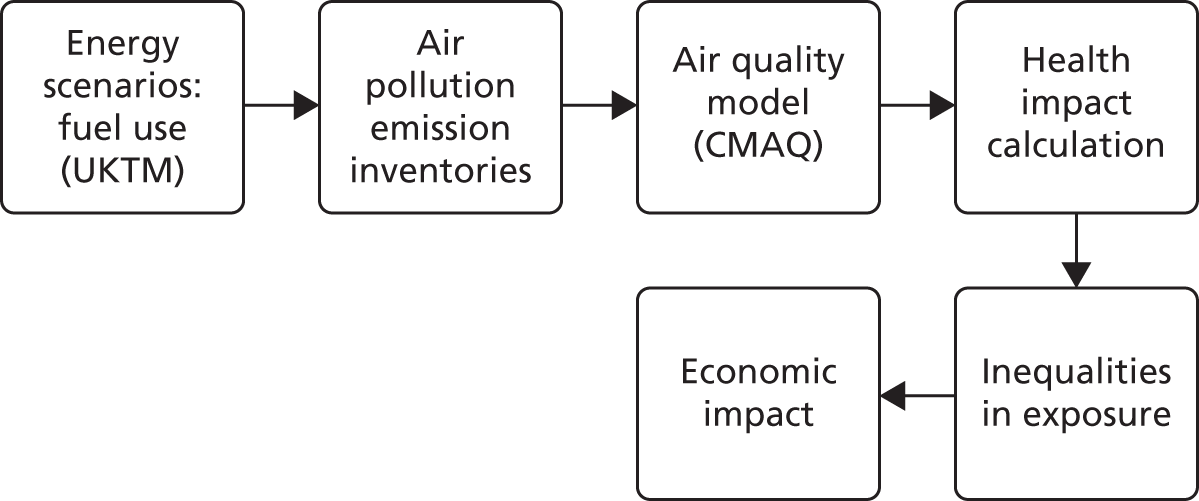
During the course of the project some of these objectives had to be modified, principally to provide a more advanced form of modelling and projection than was foreseen at the beginning of the work. This adjustment of the work packages also resulted in an increasing amount of time taken for the work and a consequent extension of the deadline for producing a final report. Nonetheless, we believe that what we have now produced represents the most sophisticated modelling of air quality concentrations and health impact assessment ever carried out in GB. A flow diagram of the work is given in Figure 1.
FIGURE 1.
Flow chart of stages in the project. CMAQ, Community Multiscale Air Quality; UKTM, The UK Integrated MARKAL–EFOM System.
We had originally intended to produce our own future scenarios using the DECC ‘calculator’, a ‘do-it-yourself’ spreadsheet tool which allows the user to produce energy scenarios which meet the CCA target for CO2-equivalent reductions. However, during the course of the project, after over a year had passed (during which time we were developing the air quality model), we made contact with the energy group at UCL, which, it transpired, had developed and was running the energy system model for the UK (UKTM), which is used by DECC (now subsumed within the Department of Business, Energy & Industrial Strategy). This presented an opportunity to produce far more robust and credible scenarios than we had previously envisaged and so we began to collaborate with the team at UCL, now co-author of the report. This, among other things, resulted in a certain delay to the project, but provided a higher quality of output. Furthermore, linking the UKTM model to an air quality model of the sophistication of the Community Multiscale Air Quality (CMAQ) model (the air quality model we used and which is described in Chapter 4) is a major step forward in modelling the impact of climate policies. This took a considerable amount of effort, but now for the first time in GB we have produced a system linking energy modelling with calculations of air pollution concentrations as opposed to the relatively easier step of linking to air pollution emissions, as several earlier studies had done.
The difference is considerable. The relative emissions from different sectors or scenarios are not necessarily directly proportional to their relative contributions to ambient pollution levels and hence population exposures and health impact. A simple example can illustrate this. A power station in a rural area with a chimney > 150 m in height will have a much smaller impact on health than a fleet of road vehicles emitting in total the same amount of pollution in an urban area. Previous analyses of air pollution impact arising from climate policies in the UK have calculated only emissions; for the first time we have produced calculations of concentrations airborne particles and direct public health impact. We have concentrated our analyses on GB rather than the UK because (1) the ultimate aim of the work was to calculate health impact from air pollution exposures and the relevant data on mortality rates were not as readily available at the required spatial resolution across the whole UK; and (2) configuring the air quality model to include Northern Ireland would have lengthened the project unduly.
Another aspect that has been somewhat time-consuming has been the development of the air quality model. We had hoped to model some cities at a fine spatial resolution, but as this is at the forefront of modelling research in the UK we were unsure of how practicable it would be. It turned out that we could run a number of major cities in GB at 20-m grid resolution using the supercomputer facility operated by the Natural Environment Research Council (NERC). We spent some time configuring the model to run on this system. The large benefits to the project came at the cost of time delays (users have to queue for run time on the NERC system). However, we have now produced the most spatially detailed concentrations and health impact ever calculated in GB.
The calculation of the impact of air pollution on health is based on numerical relationships between air pollution concentrations and the extent of adverse health outcomes such as mortality or morbidity. The relationships and indications of causality linking concentrations of PM2.5 were well established at the commencement of the project, although they were confirmed and re-emphasised by a review carried out by the World Health Organization (WHO) in the early phase of the project. However, during the course of the project it became clear that evidence was building that NO2 would need to be included in the health impact assessment, as evidence has accumulated for adverse effects of NO2 independent of those of PM2.5. Recommendations for the quantification of these impacts had been tentatively given by WHO, but during the project the advisory committee of the Department of Health and Social Care [Committee on the Medical Effects of Air Pollutants (COMEAP)] undertook to produce a report recommending an updated quantification of the impact on health from NO2. Although some interim statements were published by COMEAP, the final agreed recommendation had not appeared before the current project had been completed; we have therefore used the interim recommendations. The inclusion of NO2 in the health impact calculations thus represents a departure from the original protocol, but incorporates the most recent evidence on the adverse effects of NO2 on health. There is some uncertainty over the size of the NO2 contribution to the CRF compared with PM2.5 and other pollutants. Owing to these uncertainties we have not suggested adding the impact for the different pollutants, nor do we consider that the NO2 benefits cancel out the adverse health impact shown for PM2.5, for which the health evidence is stronger.
The other pollutant for which health effect evidence is strongest is O3, and we have quantified the impact of both long- and short-term exposures to this pollutant.
We have therefore calculated the health impact from exposures to the pollutants PM2.5, NO2 and O3.
Following the calculations of health impact, we undertook an analysis of the different exposures to air pollution in populations of differing socioeconomic deprivation and ethnicity, using the Carstairs index of deprivation together with GB-wide maps of modelled air pollution concentrations.
We had originally hoped to calculate health impact using the time–activity model of exposure which we have developed at King’s College London, in addition to the normal procedure of using ‘static’ measures of exposure from fixed-point monitoring data or from modelled grid square concentrations. We had hoped that exposure–response relationships for health outcomes might become available from research elsewhere for these new type of exposures, but in the event these have not been forthcoming so we have not been able to apply this potentially more advanced exposure assessment in this project. Nonetheless, the model promises to provide a valuable advance in health impact calculations when more detail exposure–response relationships emerge.
Chapter 2 The energy systems model and future scenarios
We used the UKTM model to develop the energy technology transition scenarios that were evaluated in this research project. The first version of UKTM was completed in 2014 as a successor to the UK MARKAL model. 35 The UK MARKAL model was a major underpinning analytical framework on long-term low-carbon technology pathways and decarbonisation costs for UK energy strategy development and legislation from 2003 to 2013. 33 Outputs and analysis from both the UK MARKAL model and, more recently, the UKTM model provided inputs for the 2003 Energy White Paper,36 the 2007 Energy White Paper37 and the 2011 Carbon Plan,32 as well as the CCC report Building a Low-Carbon Economy38 and the Fourth39 and Fifth Carbon Budgets,40 in addition to peer-reviewed academic journal publications. 33,36–43
In their 2014 paper published in Energy Research & Social Science on the operation of technical energy models within social systems, Taylor et al. 44 stated that ‘the ability of MARKAL to perform different roles for different groups has served to embed and institutionalise the model in the energy policy community’ and, furthermore, the UK MARKAL model has the ability to serve ‘different but intersecting needs of academic and policy communities over a sustained period of time’. In turn, the use of the UK MARKAL model and UKTM model has brought together communities across academia and policy, resulting in an influential network within the UK. 44
The UKTM model is based on the model generator, The Integrated MARKAL–EFOM System, which is developed and maintained by the Energy Technology Systems Analysis Program of the International Energy Agency. 45–49 The UKTM explicitly represents the technology and fuel choices across different sectors under decarbonisation objectives for the UK. These choices are made based on what is economically optimal (i.e. the least cost pathway to meet demand in each part of the energy sector), subject to a range of constraints that ensure more realistic pathways. Constraints include balancing of supply–demand, limits on technology build rates (e.g. how quickly a power plant can be constructed), technology learning rates and representation of available resources (e.g. wind, bioenergy), among others. Demand for energy services is defined externally to the model.
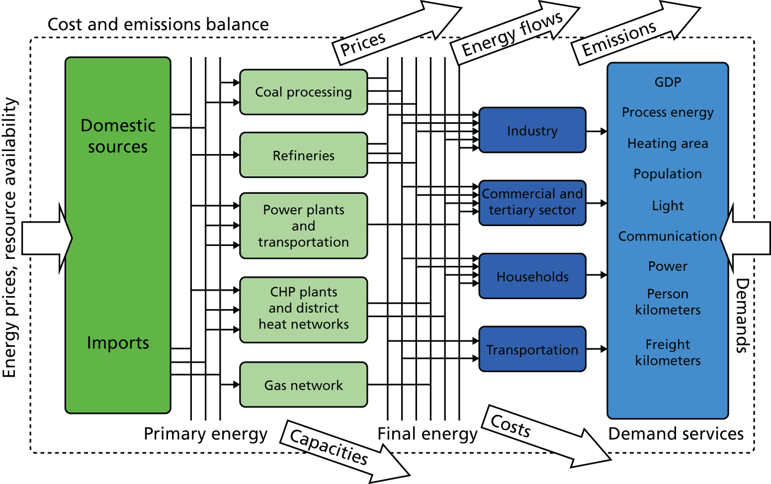
A key strength of UKTM is that it represents the entire UK energy system using a network of processes and commodity flows. In turn, the model allows for the analysis on the trade-offs between greenhouse gas reduction efforts in different parts of the energy sector, as shown in Figure 2.
Scenario development
The scenarios used in this research were developed to illustrate the possible pathways towards a decarbonised energy system in the UK through a technoeconomic lens. In this research project, the scenario outputs were then used to produce a detailed air pollution inventory and air quality analysis to help in better understanding the air quality implications of potential decarbonisation pathways.
A set of four scenarios was developed for this research project in order to assess the impact on air quality and public health in GB of possible future energy systems, as shown in Table 1 and Figure 3. Two of these scenarios (‘baseline’ and ‘reference’) were types of baseline or ‘business as usual’ scenarios, in which the 2050 target in the CCA was not achieved. The other two scenarios [low greenhouse gas (LGHG) and nuclear replacement option (NRPO)] achieved the 2050 decarbonisation target laid out in the CCA – including interim carbon budget targets – via two slightly different pathways. The difference between these two pathways lay in the assumptions made with regard to the construction of new nuclear power plants.
| Scenario | Decarbonisation ambition | Nuclear power assumptions |
|---|---|---|
| Baseline (2050) | No further carbon mitigation. Does not achieve CCA target | Nuclear phasing out (no new builds or replacements) |
| Reference (2050) | Same as baseline + £30/tonne carbon price: phased in linearly from £0 to 30 over the period of 2010–30 and then constant at £30 from 2030 onward | No constraint on nuclear beyond practical considerations (e.g. construction timelines) |
| LGHG (2035 and 2050) | 80% reduction by 2050 per CCA + achieves interim carbon budgets (through the Fourth Carbon Budget, although this is broadly consistent with the Fifth Carbon Budget) | As with ‘reference’ scenario: no constraint on nuclear beyond practical considerations (e.g. construction timelines) |
| NPRO only (2050) | Nuclear capacity capped at the current levels (i.e. no new builds, replacement only) |
FIGURE 3.
Primary energy consumption in 2050 (PJ) by scenario.

With regard to decarbonisation, the baseline and reference scenarios did not include the UK’s 2050 decarbonisation goal or interim carbon budget targets. With the baseline scenario, no carbon price was included. Conversely, the reference scenario included a £30 per tonne carbon price that was linearly phased in from 2015 to 2030 and then held constant to 2050 in order to simulate a central case in which the system moves away from the most carbon-intensive technologies (e.g. coal in the electricity sector), but long-term decarbonisation goals are not achieved.
In the remaining two scenarios (i.e. LGHG and NRPO), the energy system was required to meet existing UK decarbonisation targets for a total reduction in greenhouse gas emissions of 80% by 2050 compared with 1990 levels as stated in the CCA. Furthermore, these scenarios required that all interim targets through the Fourth Carbon Budget be met. It is noted here that, in late July 2016 (i.e. during the course of this research project), the UK government set a Fifth Carbon Budget of 1725 million tonnes of CO2 equivalents for the 2028–32 budgetary period, in agreement with recommendations from the CCC. The reduction trajectory used in this analysis is broadly consistent with this more recently agreed Fifth Carbon Budget. 42
Within these four scenarios, a key sensitivity was explored relating to the assumptions within UKTM for the nuclear power sector. The electric power sector has been responsible for most of the energy sector’s decarbonisation to date, and its future trajectory is of particular interest because of this role as the ‘first mover’. Furthermore, specifically in the context of this research, it was particularly important to understand the sensitivities surrounding nuclear power plant build as nuclear energy is an air pollution emissions-free source of power, whereas the alternatives (e.g. biomass, natural gas, coal with or without carbon capture and storage) are not. Therefore, its inclusion in (or exclusion from) the future energy technology pathway could have a potentially significant impact on the air pollution levels within the UK.
All of these scenarios examined the period to 2050 for the UK using demand drivers that relied on official population and economic growth projections and energy efficiency expectations. Primary energy consumption in 2050 by fuel type is displayed in Figure 3 for all scenarios. Also included in Figure 3 is the 2011 primary energy consumption for the UK for the sake of comparison.
Each of these scenarios was analysed using the CMAQ air quality model discussed elsewhere in this report for the year 2050 (i.e. the year the decarbonisation target is met) (see Chapter 4). Furthermore, as the UKTM output showed that domestic wood burning peaked in 2035 in the LGHG scenario, an additional air pollution emissions inventory and model run was undertaken for this interim year to understand its air quality and public health impact.
In carrying out the air quality and health impact modelling, as described in Chapters 5 and 6 of this report, we confined the analysis to GB rather than the whole of the UK, as noted in Chapter 1, even though the energy use and fuel consumption results from UKTM are presented for the UK in this section. Because of the uncertainty surrounding a future carbon price, and the fact that the emissions were not significantly different from those in the baseline scenario, we chose to restrict the air pollution concentration and health impact modelling to the baseline scenario. The wood burning increase and peak in 2035 is common to both the LGHG and the NRPO scenarios, and the overall emissions in these two scenarios are very similar, so we modelled air quality and health impact in 2035 for the NRPO scenario along with the baseline scenario for comparison. Together with the modelling of a scenario that held ‘current’ (2011) concentrations constant through to 2050, we therefore analysed a total of four scenarios in 2050 with further analyses of the baseline and NRPO scenarios in 2035.
Chapter 3 Air pollution emissions present and future
Having produced the energy scenarios from the UKTM model, the next step is to link the UKTM output with the CMAQ model. The key step in this process is to transform the UKTM energy use results into air pollution emissions, and this lies at the heart of the present project. Before describing this process, we made several improvements to the emission inventory for the current year by modifying the National Atmospheric Emissions Inventory (NAEI), as described in Current emissions in 2011: an improved inventory.
Current emissions in 2011: an improved inventory
The emissions used to model current year (2011) concentrations were derived from ECLIPSE v5a for non-UK emissions, whereas the NAEI50 and the London Atmospheric Emissions Inventory,51 and, for GB on-road traffic, used sources from the King’s College London UK emissions model. 52 ECLIPSE is a collaborative project funded under the European Union (EU) Seventh Framework Programme [(ENV.2011.1.1.2-2) climate forcing of non-United Nations Framework Convention on Climate Change gases, aerosols and black carbon]. The emission data are available at www.iiasa.ac.at/web/home/research/researchPrograms/air/Global_emissions.html (accessed 6 February 2018).
The emissions were summarised into 11 Selected Nomenclature for sources of Air Pollution Prototype (SNAP) sectors (Table 2) and were processed into gridded chemical species using speciation and temporal profiles developed in the US–EU project, Air Quality Model Evaluation International Initiative (URL: http://aqmeii-eu.wikidot.com/; accessed 6 February 2018). An additional two SNAP sectors, domestic wood burning and cooking emissions, were added, as well as SNAP 7 (road transport), intermediate volatile organic compounds (IVOCs) emissions. The temporal profiles for cooking were derived from Ots et al. 53 Biogenic emissions were estimated using the biogenic emission inventory system (version 3) model in Sparse Matrix Operator Kernel Emissions (SMOKE) v2.6. This calculation accounts for U.S. Geological Survey land cover data (URL: http://landcover.usgs.gov/; accessed 6 February 2018), high-resolution MODerate resolution Imaging Spectroradiometer (MODIS)-based land use54 and meteorological data from the weather research and forecasting (WRF) model.
| SNAP sector | Emission source description |
|---|---|
| 1 | Combustion in energy and transformation industries |
| 2 | Residential and non-industrial combustion |
| 3 | Combustion in manufacturing industry |
| 4 | Production processes |
| 5 | Extraction and distribution of fossil fuels |
| 6 | Solvent and other product use |
| 7 | Road transport (with the addition of IVOC) |
| 8 | Other mobile sources and machinery |
| 9 | Waste treatment and disposal |
| 10 | Agriculture |
| 11 | Other sources and sinks |
| 12 | Domestic wood burning |
| 13 | Cooking |
The input emissions data were provided at a range of spatial scales, from 50-km grids across non-UK Europe (ECLIPSE), down to 1-km grids in GB and traffic counts on individual roads. The link between each emissions source and the CMAQ model domains was determined by reprojecting all of the emissions data into the Lambert conformal conic projection and then intersecting each emissions database and model domain in QGIS v2.8.2-Wein.
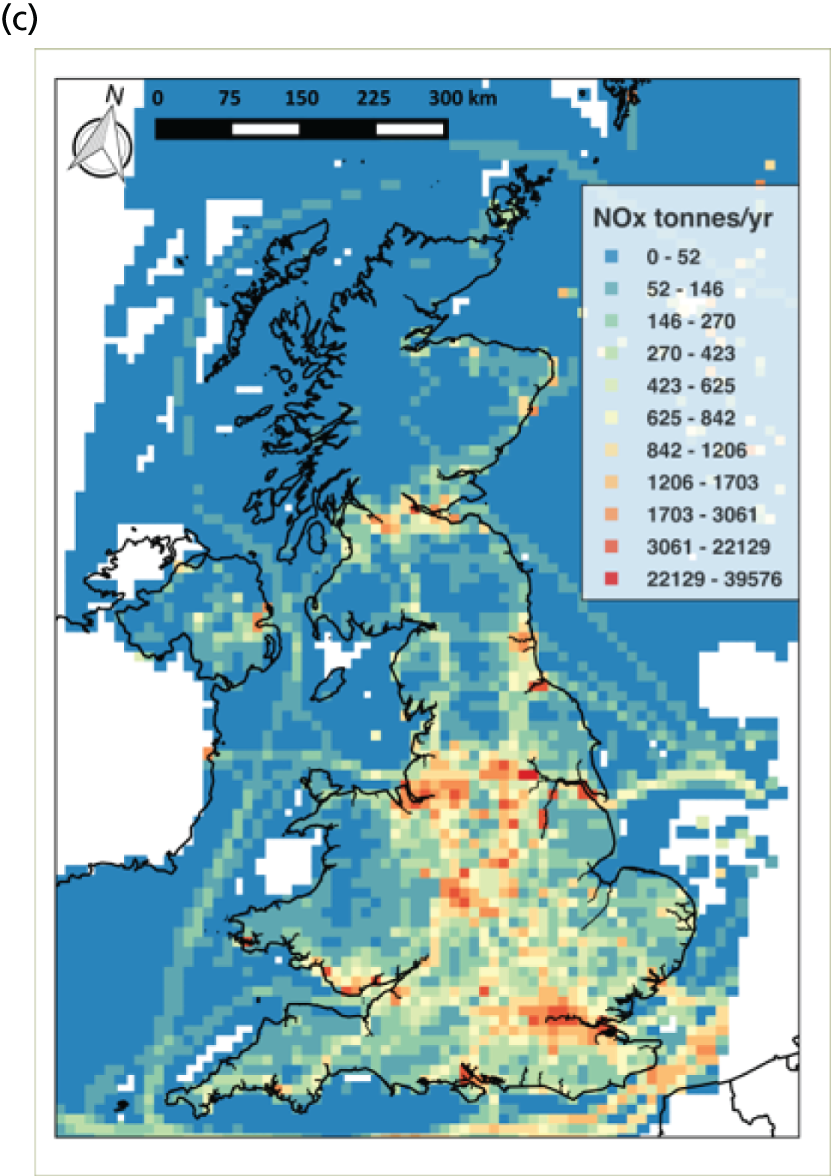
Large industrial plant emissions from ≈5000 sources in GB were taken from the NAEI database and included major power stations, iron and steel smelting and oil refineries. Details of stack heights, stack diameters, volume flow rates and release temperatures were used by SMOKE to account for the effects of plume rise. Total emissions of PM10, PM2.5 and NOx are shown in Figure 4.
FIGURE 4.
Emissions of PM10, PM2.5 and NOx in the base year (2011). (a) Emissions of PM10; (b) emissions of PM2.5; and (c) emissions of NOX.


Domestic wood burning and cooking emissions in Great Britain
A new domestic wood burning emissions inventory has been developed for the base years in 2011 and 2012 by multiplying the NAEI emissions in 2011 by a factor of 3, following the findings of a UK survey of domestic wood use. 55 In addition, the NAEI 2011 emissions also assumed that no wood burning took place in smoke control areas such as London and that, as this conflicted with the measurements of Fuller et al. ,56 who suggested that in London wood burning contributed approximately 1 µg/m3 to PM2.5 concentrations, the spatial distribution of domestic wood burning emissions was altered. The spatial distribution of wood burning emissions was undertaken by splitting the total UK emissions into 12 regions, according to the regional wood use given in Walters,55 and then distributed within each region using 1 × 1 km population data, resulting in much more domestic wood burning emissions being placed in urban areas and being more consistent with the work of Fuller et al. 56 In Europe, the domestic wood burning emissions were also scaled up by a factor of 3 following the findings of Denier van der Gon et al. 57 and hereto the emissions totals distributed using population statistics at 50 × 50 km.
Emission factors for PM2.5, PM10 and NOx from domestic wood burning have been assumed to fall in future as a result of improved stove technology and wider compliance with the EU Ecodesign Directive 2009/125/EC. 58 For 2011/12 emissions, PM emission factors remained the same as assumed in the NAEI. However, future PM emission factors were updated to reflect the emission standards in the Ecodesign Directive and assumptions about weekly use of stoves and boilers. This resulted in a reduction in the PM emission factors of 19% compared with current use. For NOx real-world emissions suggest a more realistic emissions factor of 2.3 g/kg wood burned, rather than the existing NAEI factor of 0.9 g/kg. Coupled with the increase in estimated wood use in future years, NOX from domestic wood burning increased by almost a factor of eight.
An entirely new cooking emissions inventory was developed in this project and included in the British and European emissions inventories. In GB, this was based on the methods of Ots et al. ,59 with equivalent to 320 mg/person/day added to GB PM emissions, which is four times the estimate in Paris60 and has been justified in terms of the differences in cooking methods and the relative number of food outlets in each city. The Paris figure of 80 mg/person/day was used to estimate European emissions, with the spatial distribution of the British and European cooking emissions undertaken using ward-level workday population and 50 × 50 km total population, respectively.
Diesel intermediate volatile organic compounds emissions
Another significant addition to the British and European emissions estimates has been IVOCs, not previously included in the NAEI. The magnitude of IVOC emissions has been based on measurements during the UK Clean Air for London (ClearfLo) campaign and, specifically, the findings of Dunmore et al. ,61 who showed that from the ClearfLo winter intensive observation period in London, measured concentrations of diesel IVOCs (107 µg/m3) were 3.2 times higher than petrol volatile organic compounds (VOCs) (33 µg/m3), which dominate this source in GB. Using a simple scaling factor, described by Ots et al. ,59 the existing NAEI/ECLIPSE SNAP 7 (on-road vehicle) VOCs emissions in GB and Europe were multiplied by a factor of 2.3, giving an additional GB total emission of 99.1 Gg/annum1, which is very close to the 98 Gg/annum1 total in Ots et al. 59 The same factor was used for both regions, as both have similar car fleets and proportions of diesel vehicles.
Biogenic emissions
The biogenic emissions, including VOCs, carbon monoxide (CO) and nitric oxide (NO), have been estimated based on the meteorological fields from WRF, high-resolution MODIS-based land use54 and U.S. Geological Survey soil data (URL: www.usgs.gov; accessed 6 February 2018), using the biogenic emission inventory system (version 3) model in SMOKE v2.6 (URL: www.cmascenter.org/smoke; accessed 6 February 2018).
Aircraft emissions
Aircraft emissions required specific treatment within the model to represent the emissions released at height while climbing out and approaching the airport site. For each major UK airport (Box 1), the emissions beyond the airport boundary were separated from the on-site ground-based emissions The ground-based emissions were released into the lowest model layer 14 m high, with the remaining emissions (up to 1000 m in the NAEI) being placed into layers of increasing height as the distance from the airport site increased.
-
Heathrow.
-
Gatwick.
-
Edinburgh.
-
Glasgow.
-
Newcastle.
-
Leeds.
-
Manchester.
-
Birmingham.
-
East Midlands.
-
Bristol.
-
London City.
-
Luton.
-
Stansted.
Other aircraft emissions, such as those of aircraft cruising at heights > 1000 m, were derived from the IIASA three-dimensional aircraft emission database (URL: https://tntcat.iiasa.ac.at/RcpDb) and were linearly interpolated into model grids.
It should be emphasised here that we have made no attempt to model detailed future scenarios at individual airports. Future emissions in this sector have been estimated by scaling the outputs of UKTM for the British aviation sector and using the estimates for 2030 in the NAEI projections to 2030. 62
Linking the UK Integrated MARKAL–EFOM System output to the air quality model (CMAQ)
We then built on the current year emission inventory to produce analogous inventories for the future scenarios produced by the UKTM model. The UKTM model yields energy and fuel use by a large number of user sectors, whereas the CMAQ model uses as input emissions split by just 13 SNAP sectors (see Glossary). To limit the risk of losing information available from UKTM, we converted the UKTM output via an intermediate step using the large number of nomenclature for reporting (NFR) sectors (see Glossary) and then aggregating the resulting NFR emissions back up to the 13 SNAP sectors used by CMAQ.
The soft linking of UKTM to the UK NAEI and King’s College London road traffic, IVOC and biomass (wood burning) emissions inventories allowed future emissions to be calculated separately for each emissions sector and for each pollutant in the following way:
where i = separate energy/emissions sectors, j = 2035 or 2050 and k = NOX, CO, PM10, PM2.5 and SO2.
To do this, the emissions sources within the NAEI have been linked to the relevant UKTM output. This was done by assigning each of the 370 NFR codes and associated fuel types to a SNAP code (1–1311) and one of the 129 UKTM energy sectors and fuel type predictions. This resulted in a total of 570 separate source categories, which have been scaled using UKTM to obtain 2035 and 2050 UK emissions totals for NOX, CO, PM10, PM2.5 and SO2 (note that these emission totals are UK totals rather than GB totals). Note also that hydrochloric acid was not forecast forwards and remained at the 2011 level for all scenarios and ammonia (NH3), VOC and IVOC emissions were estimated separately as described below.
After calculating future emissions by NFR sector, the total emissions were split by year and pollutant and summed, giving a ratio of emissions between the base year (2011) and future years (2035/50) for each pollutant and SNAP sector combination. The factor was then applied to the NAEI 2011 1 × 1 km emissions in GB, scaling them uniformly across GB and using the same scaling factors for GB point source emissions provided separately by the NAEI.
As a final step, the scaled 1 × 1 km emissions were converted into a format for each air pollution model run: a GB-wide 50 × 50 km emissions file, a GB 10 × 10 km emissions file and a 2 × 2 GB cities emissions file. Each of these files gives emissions (tonnes/annum) for eight pollutants and 13 SNAP sectors across regular GB spatial grids and in a Lambert conic conformal projection used by the CMAQ model.
For the emissions associated with road transport (SNAP 7), the UKTM estimates billion vehicle kilometres (Bvehkm) for each of seven vehicle types: diesel, electric, petrol, hybrid electric, hydrogen, liquefied petroleum gas and compressed natural gas. The estimates of Bvehkm have been used, in conjunction with the King’s College London’s bottom-up road transport emissions inventory,52 based on, inter alia, the King’s College London’s remote sensing measurements of vehicle emissions,63 to calculate new vehicle kilometres in each of the future years. As the increase in GB vehicle kilometres is large and the capacity of city roads is unlikely to allow such significant expansion, a two-step approach has been taken, whereby increases in larger cities such as London, Manchester and Leeds, etc., are assumed to be smaller than those elsewhere. The increase in cities was limited to those predicted in London and summarised in Table 3. Elsewhere in GB, the increase in vehicles was greater than in urban areas to maintain the increased GB Bvehkm predicted by UKTM (see Table 3). The increase in vehicle kilometres in urban areas was associated with a decrease in speed, with an elasticity of 1 meaning that a 10% increase in vehicle kilometres results in a 10% decrease in speed. Finally, vehicle stock estimates of the proportion of Euro 5/V and 6/VI plateau in the GB model from 2035 onwards, because there are, at present, no plans to go beyond Euro 6/VI vehicles. However, the type of vehicles changed markedly during this period, predicted by UKTM. A complete list of the vehicle kilometres forecasts from the UKTM model is available from the authors.
| Vehicle type | Time period | |
|---|---|---|
| 2010–30 | 2010–50 | |
| GB | ||
| Car | 1.28 | 1.49 |
| Bus and coach | 0.89 | 0.87 |
| LGV | 1.52 | 2.07 |
| Rigid HGV | 1.12 | 1.32 |
| Articulated HGV | 1.12 | 1.32 |
| London | ||
| Motorcycle | 1.04 | 1.08 |
| Taxi | 1.00 | 0.99 |
| Car | 1.06 | 1.12 |
| LGV | 1.19 | 1.38 |
| Bus and coach | 1.02 | 1.03 |
| Rigid HGV | 1.00 | 0.99 |
| Articulated HGV | 1.06 | 1.12 |
Emissions of two pollutants, NH3 and VOCs, are not well predicted using the UKTM, as fuel use from sources emitting these pollutants is a small part of the sources’ characteristics. The majority of the emission of these pollutants arises from non-combustion processes such as solvent evaporation, in the case of VOCs, and animal excretions and fertiliser use in the case of NH3. Therefore, as an addition to the UKTM estimates, we used NH3 and VOC emissions projections between 2013 and 2050 from the GAINS model – ECLIPSE version 5a, and described in the Thematic Strategy on Air Pollution report #16,64 to scale the existing NAEI emissions for NH3 and VOC. Version 5a was chosen as the forecast both is recent and includes all of the emissions reductions agreed under the member states National Emissions Ceiling Directive (NECD).
Future diesel IVOC, cooking and domestic wood burning emissions inventories were also forecast differently to those of the other NAEI sources. Diesel IVOCs, as the name suggests, are diesel vehicle-related VOCs with a higher carbon number (C10+). These higher carbon number VOCs are not routinely measured or considered within current vehicle emissions regulations and we have therefore assumed that vehicle manufacturers are not controlling them effectively. Hence, any future emissions estimate has been scaled to total diesel vehicle kilometres provided by the UKTM model.
A specific domestic wood burning emissions inventory has been developed for GB and is described in Domestic wood burning and cooking emissions in Great Britain. Future wood burning emissions are forecast using the UKTM model energy use estimates in combination with a change in PM10 and PM2.5 emissions factors, which changed from 8.2 g/kg and 7.7 g/kg, respectively, to 6.6 g/kg and 6.2 g/kg, respectively, a drop overall of approximately 20%. The latter emissions factor change is based on a weighted average emissions factor combining existing fireplaces, new stoves and highly efficient palletised wood burners. Finally, cooking emissions were scaled by the growth in population and taken from the Office for National Statistics (ONS) (URL: www.ons.gov.uk/ons/rel/pop-estimate/population-estimates-for-uk--england-and-wales--scotland-and-northern-ireland/mid-2014/sty---overview-of-the-uk-population.html; accessed 6 February 2018).
In the future scenarios we assumed that the following large power plants were closed as a result of their becoming uneconomic following the need to meet new emission limits: Kingsnorth, Ironbridge, Grain, Ferrybridge C, Tilbury B, Didcot A, Littlebrook D, Fawley, Cockenzie and Kingsnorth oil treatment plants.
Great Britain pollutant emissions in 2011 and future years
For clarity, and because these are the pollutants for which the health effects evidence is strongest, in this section we discuss only the emissions of PM10, PM2.5 and NOx; emissions of other pollutants are available on request but are omitted here.
Emissions of PM10, PM2.5 and NOx in the 2011 ‘base’ year, the baseline scenario in 2035 and 2050, the NRPO for 2035 and 2050 and the LGHG scenario for 2050 are shown in Table 4 as GB totals and in Table 5 for NOx and PM2.5 disaggregated by SNAP sector.
| Pollutant | Year (kilotonnes) | |||||||
|---|---|---|---|---|---|---|---|---|
| 2011 | 2035 | 2050 | ||||||
| LGHG | Baseline | NRPO | LGHG | Baseline | NRPO | Reference | ||
| CO | 1,975,045 | 2,128,918 | 1,370,297 | 2,158,254 | 1,157,174 | 2,941,674 | 1,182,543 | 2,886,271 |
| NH3 | 300,439 | 325,410 | 313,359 | 325,450 | 319,307 | 315,940 | 319,311 | 316,067 |
| NOX | 1,370,339 | 623,274 | 723,139 | 694,267 | 584,125 | 1,402,760 | 676,040 | 772,512 |
| PM10 | 180,517 | 228,290 | 135,790 | 230,467 | 168,000 | 185,768 | 170,294 | 178,749 |
| PM2.5 | 109,414 | 156,400 | 70,051 | 157,788 | 95,315 | 101,027 | 96,718 | 99,648 |
| SO2 | 474,080 | 148,746 | 194,314 | 149,446 | 151,231 | 227,522 | 153,584 | 196,500 |
| VOC | 949,152 | 941,445 | 829,542 | 947,133 | 910,310 | 850,394 | 1,051,541 | 839,544 |
| IVOC | 99,117 | 1209 | 22,842 | 1285 | 0 | 6541 | 0 | 2216 |
| CO2 (MtCO2e) | 553 | 304 | 494 | 305 | 208 | 488 | 207 | 404 |
| Pollutant | SNAP sector | Year (kilotonnes/annum) | |||||||
|---|---|---|---|---|---|---|---|---|---|
| 2011 (base case) | 2035 | 2050 | |||||||
| LGHG | Baseline | NRPO | LGHG | Baseline | NRPO | Reference | |||
| NOx | Energy combustion | 308,535 | 71,318 | 145,335 | 81,663 | 88,247 | 150,935 | 107,267 | 106,134 |
| Non-industrial | 55,613 | 34,499 | 33,241 | 92,895 | 23,068 | 35,544 | 89,482 | 35,104 | |
| Manufacturing | 112,452 | 43,076 | 87,705 | 46,354 | 38,199 | 777,667 | 44,512 | 192,820 | |
| Production processes | 14,988 | 12,038 | 10,916 | 12,001 | 34,155 | 13,869 | 34,109 | 14,067 | |
| Extraction/distribution | 61 | 4 | 4 | 4 | 118 | 6 | 332 | 0 | |
| Solvent use | 0 | 0 | 0 | 0 | 0 | 0 | 0 | 0 | |
| Roads | 378,416 | 43,918 | 54,400 | 42,739 | 29,094 | 56,974 | 29,102 | 56,380 | |
| Other mobile | 491,956 | 388,614 | 389,552 | 388,702 | 360,049 | 361,894 | 360,018 | 361,708 | |
| Waste | 1194 | 1791 | 1106 | 1840 | 1127 | 1242 | 1165 | 1136 | |
| Other | 450 | 693 | 693 | 693 | 693 | 693 | 693 | 693 | |
| Residential wood burning | 6675 | 27,322 | 185 | 27,376 | 9375 | 3936 | 9361 | 4470 | |
| PM2.5 | Energy combustion | 4239 | 933 | 1209 | 1032 | 1049 | 1364 | 1214 | 1003 |
| Non-industrial | 14,164 | 16,026 | 11,948 | 17,096 | 11,661 | 13,506 | 12,855 | 13,523 | |
| Manufacturing | 4986 | 6053 | 7344 | 6092 | 2224 | 22,176 | 2284 | 19,536 | |
| Production processes | 5134 | 4185 | 4148 | 4186 | 4047 | 3928 | 4048 | 3948 | |
| Solvent use | 1388 | 1383 | 1383 | 1383 | 1383 | 1383 | 1383 | 1383 | |
| Roads | 21,904 | 15,531 | 15,636 | 15,519 | 18,173 | 18,524 | 18,173 | 18,518 | |
| Other mobile | 20,449 | 15,747 | 15,762 | 15,757 | 15,193 | 15,327 | 15,193 | 15,329 | |
| Waste | 3456 | 10,946 | 1097 | 10,982 | 4398 | 2476 | 4419 | 2609 | |
| Agriculture | 2017 | 837 | 837 | 837 | 905 | 905 | 905 | 905 | |
| Other | 1638 | 1576 | 1576 | 1576 | 1576 | 1576 | 1576 | 1576 | |
| Cooking | 7434 | 8607 | 8607 | 8607 | 9116 | 9116 | 9116 | 9116 | |
| Residential wood burning | 22,604 | 74,576 | 505 | 74,722 | 25,590 | 10,745 | 25,552 | 12,202 | |
Turning to the baseline scenario, the fundamental premise was that there would be no further carbon mitigation beyond those measures already in place. It should be noted that the CCA target was not included as a constraint and, consequently, the 80% emission reduction target in the CCA is not achieved: the overall reduction in CO2 equivalents in 2050 is 39%. Nuclear power generation is phased out and there is no carbon price to influence energy options or emissions. The output from UKTM in 2050 shows a decrease in primary energy consumption from 9355 PJ in 2010 to 7091 PJ in 2050. A significant part of this decrease is because of the decline in nuclear power generation from 562 PJ in 2010 to 73 PJ in 2050. Biomass (wood) use shows a modest increase from 288 PJ to 307 PJ, whereas natural gas use decreases only by a small amount, from 3748 PJ to 3515 PJ, and oil use shows a larger decrease, from 3349 PJ to 2653 PJ.
The scenario includes large increases in energy use for combined heat and power (CHP) in the industrial and residential sectors, fuelled by biomass and natural gas. In the industrial and residential sectors, the use of biomass for CHP increases from 8.17 PJ and zero, respectively, in 2010 to 148.17 PJ and 21.76 PJ in 2050. Natural gas consumption for CHP in the industrial sector shows a modest increase from 143.9 PJ in 2010 to 157.76 PJ in 2050, whereas the residential sector shows a large relative increase from 3.5 PJ in 2010 to 77.69 PJ in 2050. These changes contribute to the fact that NOx emissions in 2050 are higher in the baseline scenario than in the other scenarios.
The LGHG scenario, by contrast, shows a large increase in biomass consumption in 2035 (1089 PJ, compared with 289 PJ in 2010), before decreasing in 2050 to 932 PJ, still about three times higher than in the base year. This is the main reason for the large increase in PM2.5 and PM10 emissions in 2035 shown in Tables 4 and 5. By 2050 biomass use is still above that of the base year, but the increase in PM emissions from this source is now offset by reductions in other sectors, notably transport, as the majority of the road vehicle fleet is projected to be electric. However, the electrification of the vehicle fleet will reduce only exhaust emissions of PM10 and PM2.5; non-exhaust emissions from tyre, brake and clutch wear will not fall unless action is taken to reduce emissions from this source. It is possible that technologies such as regenerative braking on electric vehicles may act to mitigate these non-exhaust emissions, but there is little evidence at present to allow us to quantify this, so we have assumed that emission factors stay at present levels out to 2050. In the LGHG scenario, vehicle activity is projected to increase substantially from 2010 to 2050, by roughly 50% for cars and heavy goods vehicles and by roughly a factor of 2 for vans. With constant non-exhaust emission factors this represents a substantial relative increase in non-exhaust emissions and hence concentrations from this source. The health implications of this are discussed in Chapter 5. The LGHG scenario has the largest contribution of nuclear power to the energy mix in 2050, at 2454 PJ, but the air pollutant emission benefits of this are offset by the relatively large contribution from biomass.
The nuclear replacement scenario seeks to limit nuclear power station build in that existing nuclear stations will be replaced but no additional new ones will be built. The contribution of nuclear power to the energy mix in 2050 is therefore much less than in the LGHG and reference scenarios and is similar to the contribution in PJ currently. The biomass contribution is also relatively high and similar to that in the LGHG scenario, and both the LGHG and the nuclear replacement scenarios show a large peak in biomass use in 2035, at 1089 PJ and 1126 PJ, respectively. This suggests that both scenarios will have potentially detrimental effects on air quality and public health, and this will be explored in Chapters 5 and 6 of this report.
Non-Great Britain emissions
As well as GB emissions, we need to take into account the contribution of sources in the rest of Europe. For emissions of pollutants from these countries we have used data from the ECLIPSE project. We used version 5a, which dates from July 2015 and incorporates current agreed legislation (the ‘CLE’ scenario) on air quality and climate change in the EU, currently agreed together with emission projections carried out by IIASA following discussions with the individual member states of the European Union during the revision of the NECD. Emission totals for non-UK Europe are shown in Table 6.
| Pollutant | Year (kilotonnes/annum) | % reduction 2011–50 | ||
|---|---|---|---|---|
| 2011 | 2030 | 2050 | ||
| CO | 65,730 | 52,684 | 50,304 | 23 |
| NH3 | 6258 | 6607 | 7025 | –12 |
| NOx | 18,627 | 14,015 | 13,231 | 29 |
| PM10 | 7705 | 7346 | 7757 | –0.7 |
| PM2.5 | 5845 | 5387 | 5435 | 7 |
| SO2 | 13,815 | 10,256 | 11,671 | 16 |
| VOC | 15,767 | 12,464 | 12,303 | 22 |
As it is impossible to predict, with any degree of confidence, future emission reduction agreements between countries in the EU and beyond, we made no attempt to model any more ambitious scenarios for which projections were made in the ECLIPSE project. The non-UK emission projections may therefore be pessimistic; the modelling undertaken in this project was largely carried out while the NECD was being negotiated and, at the time of writing, the final position had still to be formally agreed. The revised NECD [discussed in Linking the UK Integrated MARKAL–EFOM System output to the air quality model (CMAQ)] and further measures in countries following the United Nations Framework Convention on Climate Change Paris Agreement on climate change may well lead to further reductions than it has been possible to include here, so air quality in GB may improve more than we have currently projected. This could be the subject of further research using the models developed here.
These non-UK emissions will have the biggest influence on GB concentrations of PM2.5, PM10 and O3. For NO2, GB emissions will be dominant and the policies and measures enacted in response to air quality legislation and the measures put in place to meet the CCA targets will largely determine concentrations of NO2.
Of the precursors of PM2.5, the reductions in NOx are the largest (≈29%), with SO2 reductions of ≈16% by 2050. The other important precursor, NH3, is projected to increase by a small amount. This continues the poor performance regarding NH3 reductions in Europe, which have already lagged significantly behind those of other pollutants over the past few decades. Emissions of VOCs will be important for peak concentrations of O3 in photochemical episodes, and total European emissions are projected to decrease by ≈22% out to 2050.
However, the non-UK emissions in Table 6 include emissions from Eastern Europe, countries some distance from GB with relatively small influence on GB concentrations of PM2.5 and O3. For PM2.5 and O3, emissions of NOx, SO2, VOCs and NH3 in GB’s nearest neighbours (France, Germany, Belgium, the Netherlands and Poland) will be the most important, as will those from shipping,65 and these are shown in Table 7.
| Pollutant | Year (kilotonnes/annum) | % reduction 2010–50 | ||
|---|---|---|---|---|
| 2010 | 2030 | 2050 | ||
| NOx | ||||
| Neighbours | 3759 | 1789 | 1529 | 59 |
| Shipping | 4062 | 3240 | 2531 | 38 |
| SO2 | ||||
| Neighbours | 1923 | 1026 | 829 | 57 |
| Shipping | 2358 | 1617 | 1095 | 54 |
| NH3 | ||||
| Neighbours | 1861 | 1803 | 1806 | 3 |
| Shipping | – | – | – | – |
| VOCs | ||||
| Neighbours | 3480 | 2695 | 2439 | 30 |
| Shipping | 151 | 143 | 131 | 13 |
| PM2.5 | ||||
| Neighbours | 1044 | 781 | 662 | 37 |
| Shipping | 288 | 210 | 147 | 49 |
Several features are apparent from Table 7. First, the reductions in PM2.5 and O3 precursors are greater in GB’s near neighbours than in the whole of Europe (including Eastern Europe). Second, although shipping is projected to make significant reductions in emissions out to 2050, this source remains large and by 2050 is projected to be larger than the land-based emissions from GB’s neighbours. The third point of importance is the very small projected reduction in NH3 emissions, which will limit the reductions in PM2.5 concentrations in GB in future years. As noted elsewhere in this report, the lack of large reductions in NH3 emissions has represented a major challenge to most European countries over the past few decades. The recently agreed NECD, however, does suggest that further action should be forthcoming: the agreement on NH3 is for a 19% reduction by 2030 on a 2005 base for the 28 EU member countries as a whole and reductions of 13–29% for GB’s near neighbours. This figure is not directly comparable to the figures in Table 7 and, as the NECD was only very recently agreed, time has not permitted a full analysis. However, the commitments in the new directive suggest that the NH3 emission reductions used here may be pessimistic. The corresponding reductions in NOx, SO2 and primary PM2.5 range from 39% to 69%, from 53% to 77% and from 39% to 58%, respectively. Further work would be required to compare these commitments with the projections we have used based on the ECLIPSE project. As noted above, there should be a degree of consistency between the two as the ECLIPSE project involved detailed discussions with EU member states, but clearly the two will not necessarily match.
Chapter 4 The air quality model, description and evaluation
In modelling air quality in GB, we used the CMAQ model, which is widely used across the world. It is an open-source mathematical model supported with regular updates by the United States Environmental Protection Agency (US EPA), using a considerable degree of feedback from the user community worldwide. The model splits the atmosphere into three-dimensional grid cells and calculates the way that air pollutants are carried by the winds, the way they dilute and disperse and the way they react chemically in the air. The computer power requirements are considerable and we eventually ran the model on the NERC supercomputer system. The version of the model which we used in this study is CMAQ volatile basis set (VBS) version 5.0.2. CMAQ and the Atmospheric Dispersion Modelling Software (ADMS) have been coupled together to give a model we describe as CMAQ-Urban,66 which outputs air pollution concentrations across GB every 10 km, 2 km or 20 m, for every hour of 2011 and 2012 for model evaluation and in 2035 and 2050 for the different climate policy scenarios.
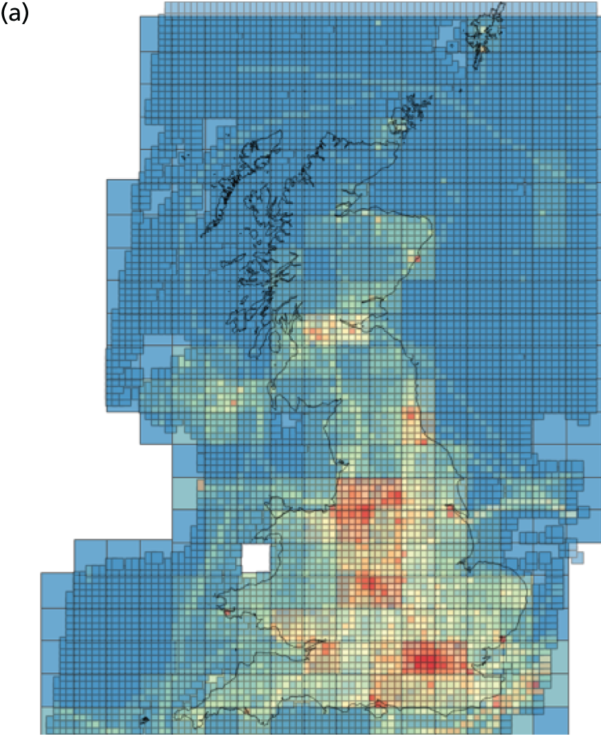
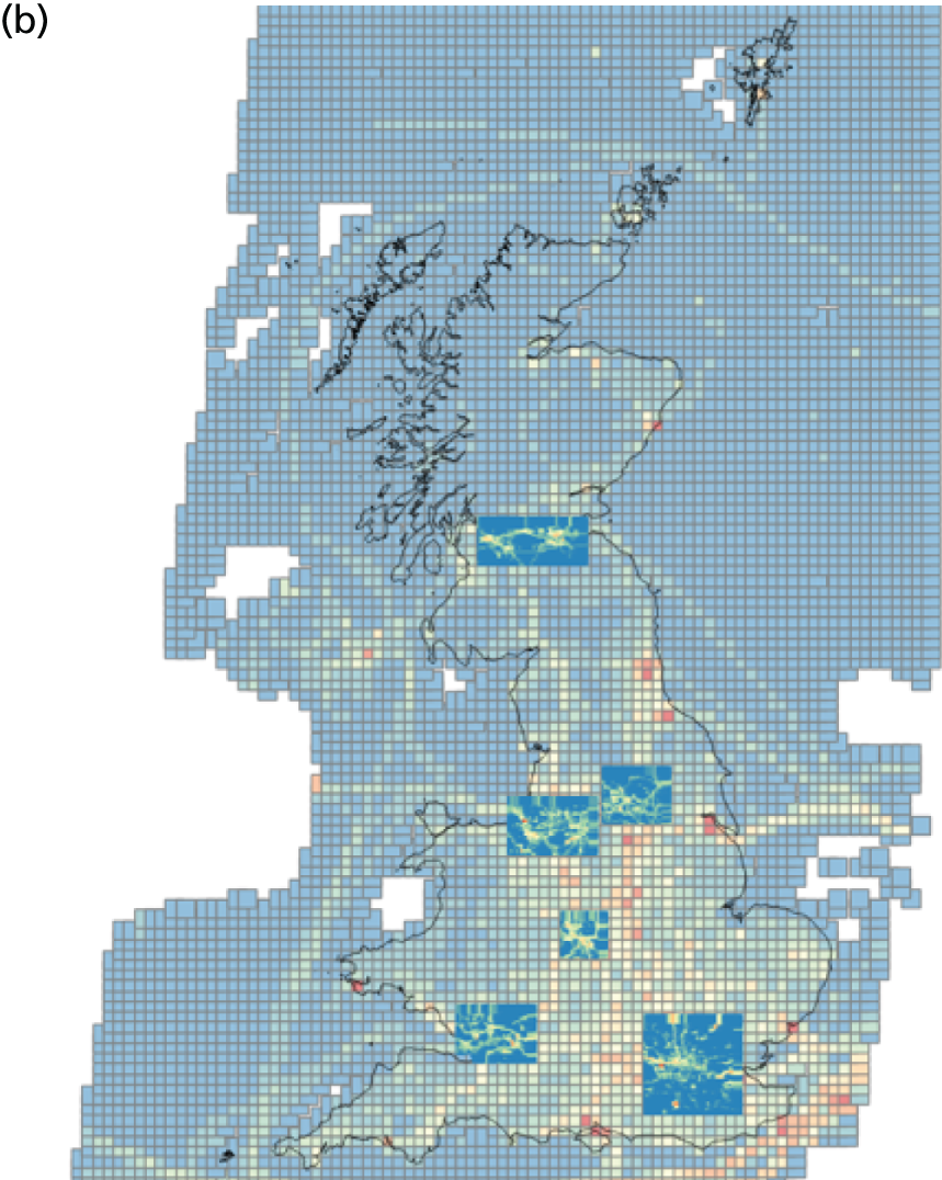
The CMAQ model is driven by meteorological fields from the WRF model v3.6.167 and was set up using 23 vertical layers of the atmosphere, with seven layers under 800 m and the top layer ≈15 km above the ground. Four horizontal nesting levels were used, downscaling from 50-km grids over Europe to 10-km grids over GB and 2-km and 20-m grids over cities in GB (London, Bristol/Swansea/Cardiff, Birmingham, Liverpool/Manchester, Leeds and Glasgow/Edinburgh) (Figure 5).
FIGURE 5.
Model nesting levels, example NOx (2011). (a) Plot 50 km to 10 km, all sources; and (b) plot 10 km to 2 km/20 m, mobile sources.
The lateral boundary conditions for 2012 WRF simulations were taken from the National Centers for Environmental Prediction Final Operational Model Global Tropospheric Analyses with 6-hour interval and 1° grid resolution. The WRF physics schemes include the rapid radiative transfer model longwave radiation scheme, the Dudhia shortwave radiation scheme,68 the Kain–Fritsch cumulus parameterisation scheme,69 the WRF single-moment six-class microphysics scheme,70 the Pleim-Xiu surface-layer scheme,71 the rapid update cycle land-surface model72 and the asymmetrical convective model version 2 for the planetary boundary layer. 73 Throughout the WRF simulations, grid analysis nudging of temperature, wind speed and water vapour mixing ratio has been applied within, and above, the planetary boundary layer, with nudging coefficients of 3 × 10⁻⁴/second.
The meteorological fields for 2011, 2035 and 2050 were derived from WRF simulations with configurations described above. For consistency across scenarios, the model was driven by the lateral conditions from the global coupled carbon climate Earth system model developed at the US Department of Commerce, National Oceanic and Atmospheric Administration, Geophysical Fluid Dynamics Laboratory. 74 The data were the products of the fifth phase of the Climate Model Intercomparison Project75 and are available from the Geophysical Fluid Dynamics Laboratory data portal (URL: http://nomads.gfdl.noaa.gov; accessed 6 February 2018). The variables used for WRF simulations include two-dimensional near surface and three-dimensional data (air temperature, U and V wind, specific humidity and air pressure), sea level pressure, surface and sea surface temperature, temperature and water content of soil.
The CMAQ v5.0.2 model with the VBS scheme76 (URL: www.airqualitymodeling.org/index.php/Main_Page; accessed 6 February 2018) was set up using the same vertical and horizontal grid structure as for WRF. Atmospheric chemistry was simulated using the CB05-TUCL gas-phase chemistry mechanism and AE6 aerosol mechanism. 77,78 Chemical boundary conditions were derived from the global chemical transport model MOZART-479 and the National Oceanic and Atmospheric Administration, Geophysical Fluid Dynamics Laboratory AM3 model80 (URL: www.gfdl.noaa.gov/atmospheric-model/; accessed 6 February 2018), which provided 14 pollutant species [CO, NOX, O3, hydroxyl, SO2, nitric acid and VOCs, sulphate, nitrate, ammonium, black carbon, primary organic aerosol (POA) and secondary organic aerosol (SOA) and sea salt]. Sea salt emissions are driven by the metrological fields from WRF and are calculated within the CMAQ model.
The ADMS roads model (v2.3)81 was used to describe the near-field dispersion from roadways in CMAQ-Urban, using the hourly meteorological inputs (wind speed and direction, temperature, surface sensible heat flux and planetary boundary layer height) predicted from the WRF model. 66 The near-road chemistry was simulated using a simple chemical scheme described by Carslaw and Beevers. 82 The reaction rates and photodissociation rates were taken from a photolysis rates processor,83 part of the CMAQ run, and the time of flight from road sources, estimated each hour as a concentration-weighted average at each receptor location, assuming a straight line between source and receptor and using WRF wind speed at 10 m height.
The CMAQ volatile basis set scheme
Modelling the concentrations and composition of atmospheric particles is a complex task and the science is continuallly developing. An important part of improving the model’s predictive capability for PM2.5 and PM10 was the addition of a number of emissions sources for the UK and Europe, including diesel IVOCs and organic aerosol (OA) from cooking, based on aerosol mass spectrometry measurements, and a large increase in domestic wood-burning emissions. Another important improvement in the chemical mechanism in CMAQ was the use of the VBS scheme84,85 to account for the chemical ageing and volatility of organic gases and aerosols. OAs comprise POA emitted from sources such as motor vehicles and SOA formed in the atmosphere from gas phase precursors. Briefly, a proportion of POA evaporates on dilution to ambient conditions and then photo-oxidises to give SOA. 86
Gas-to-particle partitioning of POA emissions depends on its volatility distribution and has been traditionally assumed to be non-volatile. However, Robinson et al. 86 found that additional diesel IVOCs were emitted, contributing between 1.5 and 3 times the POA emission. The VBS scheme aims to represent this more realistic OA behaviour by representing emissions in volatility bins, ranging from those that are non-volatile at ambient conditions to semivolatile organic compounds (SVOCs) (i.e. that partition between particle and gas phase, and IVOCs that start in the gas phase). The VBS also includes oxidation or ageing processes, which, starting from SVOC and IVOC, produce compounds of lower vapour pressure and generate substantial amounts of SOA over time scales from hours to days. Use of VBS increases the amount of regional SOA in urban areas, a different split between POA and SOA, although not necessarily higher OA levels than assuming non-volatile POA. 86
Representing organic emissions in the CMAQ model
Within air pollution models it is impossible to individually represent the thousands of organic compounds that exist, with current emissions inventories reporting only highly volatile VOCs emissions (mainly petrol emissions) and lower volatility species emitted as particles. Organic compounds with low/intermediate volatility (SVOCs and IVOCs) are difficult to quantify; therefore, this is not routinely undertaken.
The model underestimation of OA highlights the need for measurements of SVOCs and IVOCs and for these species to be reported in emissions inventories. Although both petrol87,88 and diesel vehicles89 have been reported as the most important for the generation of SOA, here we have introduced additional diesel-related IVOC emissions, derived directly from the ClearfLo measurement campaign in 201290 at an urban background site in Kensington, London. 61
The CMAQ VBS treats four distinct basis sets or OA groups: primary anthropogenic OA (hydrocarbon-like OA or POA), anthropogenic SOA, biogenic SOA and primary biomass burning aerosols. Five bins, classified by the saturation concentrations (C*) of 0.1, 1, 10, 100, 1000 µg/m3, were used to represent volatility bins in each of the basis sets. C* ≤ 0.1 represents non-volatile particles. Although the standard CMAQ AE6 scheme assumes POA as non-volatile, the VBS scheme treats it as semivolatile POA. Primary SVOCs undergo atmospheric ageing/oxidation in gas phase by reacting with hydroxyl radical (with a rate coefficient of 4.0 × 10⁻¹¹ cm3/molecule/second),86 resulting in a shift from primary SVOCs (POA) to secondary SVOCs (SOA) into the next lower volatility bin and a mass increase of 10%.
The mass of IVOC emissions (see Table 4) has been introduced into the CMAQ model using n-pentadecane (C15H32) as a surrogate, as it is representative of diesel emissions and the rate constant of the unmeasured organic compounds. Within this study, a background OA of 0.4 µg/m3 was also used to represent the missing source (e.g. oceanic sources or spores). 53
CMAQ-Urban outputs
The CMAQ model was run for GB at 10 km, and in major cities at 2-km and 20-m, resolution with all runs nested within the larger European domain. The CMAQ predictions of hourly air pollution at 2 × 2 km were downscaled to a fixed 20 × 20 m grid using the bilinear interpolation method described by Shaoa et al. 91 The CMAQ hourly concentrations are smoothly varying in space for each hour, and this limits the error introduced through the interpolation step and allows a direct match with the ADMS model outputs. The ADMS model predicts concentrations of primary pollutants, which are then added to the CMAQ background concentrations and for NO, NO2, and O3 close to roads, using a simple chemistry scheme applied for 2011/12. 82
The coupling of the local-scale model with the outputs of CMAQ at a 2-km scale results in a double-counting error as a result of local road emissions being counted in the CMAQ background concentrations. This has been resolved at model run time in the following way. Using the contribution to air pollution from each road separately, the equivalent road emissions are mixed into the 2 × 2 km CMAQ grid to estimate the double counting concentration for each hour. This is repeated for each road in turn as the model run is under way and allows a correction of the background CMAQ concentration prior to the inclusion of the local road contribution and the application of the chemistry scheme.
We ran CMAQ at 2-km resolution in urban areas because the finer the grid size the better the model is at identifying pollution ‘hot spots’ which are important for health impact calculations. As discussed in Chapter 5, although we report concentrations at 20 m resolution in the major British cities, we were unable to use these results for health impact calculations as the relevant health data are not available at such fine spatial resolution.
Chapter 5 Air quality model evaluation
The results from the CMAQ-Urban model were then analysed using the methods described in the UK Department of the Environment, Food & Rural Affairs model evaluation protocol and reported using the ‘OpenAir’ software (University of Leeds, Leeds; King’s College London, London). In the model evaluation, use was made of 80 monitoring stations from the UK and London monitoring networks (URL: www.londonair.org.uk/LondonAir/Default.aspx; accessed 16 February 2018), including 22 urban background, 13 suburban, 38 roadside and seven kerbside sites. Statistical measures of model performance included the fraction of modelled values within factor of two of the observations, the mean bias and normalised mean bias, the root-mean-square error and the correlation coefficient (r). Diagnostic evaluation used modelled and measured concentrations, averaged by hour of the week and month of the year.
CMAQ-Urban model evaluation in 2011/12
The purpose of model evaluation is to establish the suitability of the CMAQ-Urban model for predicting present-day concentrations of NO2, PM2.5, PM10 and O3, without the need for bias correction using measurements. This is important to establish as models that require correction through assimilation with ambient data have the potential to introduce bias into any future predictions and are therefore less well suited for policy development.
There have been two major development areas required in establishing suitable model performance for predicting PM2.5, PM10, O3 and NO2: (1) the adoption of more sophisticated modelling of OAs, including the generation of secondary species, using the now well-established VBS scheme in CMAQ; and (2) the development of emissions not currently available in GB, including diesel-generated IVOCs, organic cooking emissions (based on aerosol mass spectrometer measurements) and an update of the GB biomass burning emissions inventory (based on the most recent surveys of wood use and emissions factors from the UK and Europe). Furthermore, as NO2 is a problem pollutant close to roads in GB, and NOX and NO2 emissions are important for predicting O3, improvements have been made to vehicle emissions factors using UK remote sensing data within the King’s College London UK NOX and NO2 traffic emissions model. Finally, it is expected that non-exhaust PM emissions are likely to dominate over exhaust emissions in the future and so the King’s College London non-exhaust emissions factors have also been used in the traffic emissions model.
The evaluation presented here includes an assessment against measurements in 2012 using the CMAQ model results at a 10 × 10 km spatial scale. This scale is commensurate with the PM2.5/PM10 and O3 outputs from the future climate scenarios considered. However, as NO2 and non-exhaust PM10 is a much more localised and traffic-related problem, a further evaluation has been made against ambient measurements using the CMAQ-Urban model at a 20-m spatial scale, including at roadside and kerbside sites. This level of spatial resolution represents the most detailed modelling of GB and its major urban areas ever carried out.
Performance of CMAQ-Urban for annual means
In this section we discuss the comparison between 10-km annual average predictions of PM2.5, PM10 and O3 against GB ambient measurements. We use the 10-km resolution here as the concentrations of these pollutants show less spatial variability than NO2. We report the 20-m urban resolution model results for NO2 in Chapter 6. To understand the annual performance of the CMAQ-Urban model predictions, an evaluation process has been undertaken against fixed-site measurements from the Department of the Environment, Food & Rural Affairs’ Automatic Urban and Rural Network and from the London Air Quality Network, as shown in Figure 6. This has been based on our experience of model evaluation from both phases of the UK model intercomparison exercise. 92 The focus of the analysis has been on the comparison between 10-km predictions at rural, suburban and urban background sites, as the spatial scale of pollutants close to sources, such as at roadside and kerbside sites, renders them unsuitable for comparison, with a separate comparison (NO2 and PM10) close to roads.
FIGURE 6.
Automatic Urban and Rural Network and London Air Quality Network measurement sites (green circles) used in the model evaluations; 10-km grid emissions (coloured), over which model concentrations are predicted; and the road network (black lines) used for the CMAQ-Urban model.

The results in Figures 7 and 8 show that the model predicts background concentrations well across GB and, in concert with the performance statistics in Table 8, has very little overall bias (normalised mean bias –2%) and a good correlation coefficient of r = 0.8. Concentrations at some monitoring sites are overpredicted, such as rural Rochester and Glazebury and suburban London Eltham, whereas others such as urban background Fort William/Aberdeen, Plymouth and Edinburgh are underpredicted. It is important not to overinterpret these data as the model predicts averages over 10-km grid squares compared with measurements at a single point and this leads to the possibility of increased variance in the site-by-site comparison. The small NO2 bias is despite a –23% underprediction of NOX which is associated with the underprediction of emissions from road transport (this has been well documented in the recent literature63). The consequence of this is that O3 is overpredicted and in this case by the same proportion (+23%), although not in absolute terms (–8 µg/m3 for NOX and +10 µg/m3 for O3). However, as NOX, NO2 and O3 are chemically linked, this suggests that the model’s chemistry is working well. The correlation coefficient of the model for O3 (r = 0.82) also points to good model performance. Other important determinants of the O3 in the CMAQ model include model boundary conditions. In this run we have used MOZART-4, which provides good O3 performance, but still contributes to model uncertainty and positive bias.
FIGURE 7.
Scatterplots of 2012 annual average modelled vs. measured NO2 concentrations (µg/m3) at GB sites.
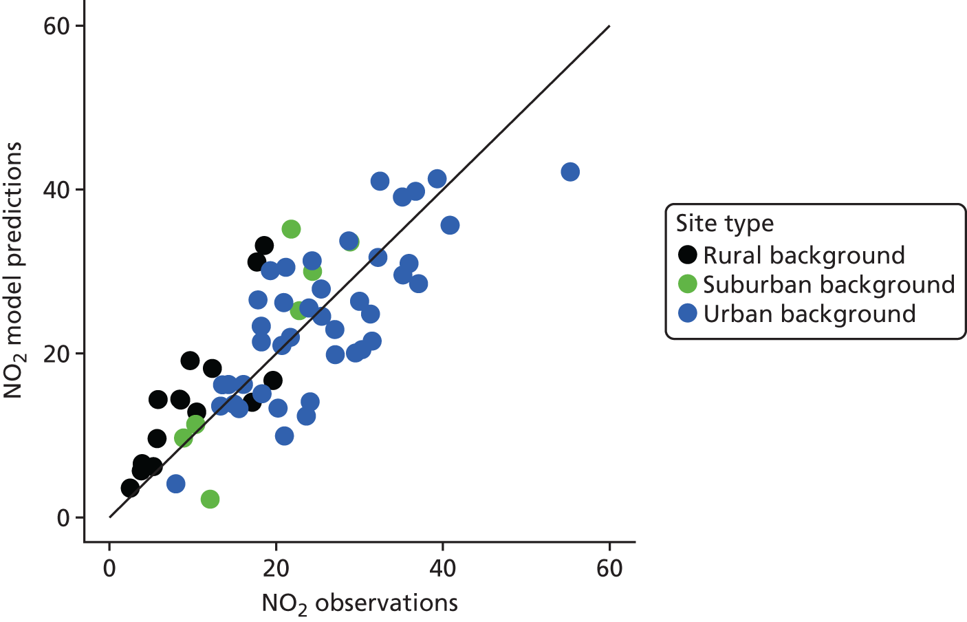
FIGURE 8.
Scatterplots of 2012 annual average modelled vs. measured O3 concentrations (µg/m3) at GB sites.
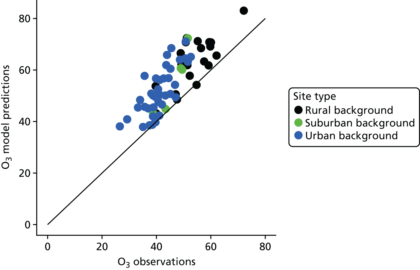
| Pollutant | n | Statistic | |||||||
|---|---|---|---|---|---|---|---|---|---|
| FAC2 | MB | MGE | NMB | NMGE | RMSE | r | IOA | ||
| PM2.5 | 35 | 1.0 | –1.1 | 1.6 | –0.09 | 0.13 | 2.1 | 0.72 | 0.58 |
| PM10 | 31 | 1.0 | 0.5 | 3.8 | 0.03 | 0.24 | 5.0 | 0.31 | 0.33 |
| NO2 | 64 | 1.0 | 0.5 | 5.3 | 0.02 | 0.25 | 6.6 | 0.80 | 0.68 |
| O3 | 65 | 1.0 | 10.3 | 10.3 | 0.23 | 0.23 | 12.0 | 0.82 | 0.25 |
| NOX | 64 | 0.9 | –7.9 | 10.9 | –0.23 | 0.32 | 14.5 | 0.79 | 0.64 |
| PM10 SS | 31 | 1.0 | –1.3 | 2.6 | –0.10 | 0.19 | 3.3 | 0.63 | 0.54 |
The model also performs well for PM2.5 (Figure 9), with good agreement across a range of concentrations from 5 to 17 µg/m3. Correlation coefficients are lower than for NO2 and O3, at r = 0.72, with a small bias of –9% (which again represents good model performance). Some sites are underpredicted, however, including Aberdeen, Leeds and Sheffield centre and Eastbourne, and, although care is needed not to overinterpret the results, all are at urban background locations and may reflect the need for more detailed spatial modelling to correctly represent local sources. At first sight, PM10 is more problematic as there is a reduction in the value of r (0.31), albeit still with only a small positive bias overall of 3% (Figure 10). Four sites in particular are grossly overpredicted (including a rural site); these are Newport, Hull Freetown, Rochester Stoke and Portsmouth. As Rochester also features in the PM2.5 plot and is underpredicted, this suggests an overprediction of coarse PM (PM10–PM2.5) and, as all four of the sites are coastal, points to the overpredictions of sea salt. Analysis of the contribution of sea salt at the four locations shows that Rochester is highest of all sites at 13.7 µg/m3, Portsmouth is third highest (13.3 µg/m3), Hull is fifth highest (11.2 µg/m3) and Newport is 14th (8.3 µg/m3). The influence of sea salt on the model’s performance is reinforced by removing the modelled sea salt estimate from the model forecast and a typical value of 2.5 µg/m3 from the observation, and reanalysing the results at the 31 PM10 sites (see PM10 SS in Table 8). The scatter reduces (not shown) and the grossly overpredicted sites fall much closer to the 1 : 1 line, which results in an r-value of 0.63 and a bias of –10%, suggesting that predictions of anthropogenic PM10 sources are well represented in the model. Finally, the fact that approximately 23 of the British Automatic Urban and Rural Network sites are close to the coast, yet only four showed significant influence from high predictions of sea salt, suggests that this is a local coastal phenomenon and of less importance for the majority of GB. On closer inspection, the four sites are a number of kilometres from the coast but within a 10-km square that has a significant ‘surf zone’ within it. Again, more spatially detailed modelling around the British coasts alongside coastal PM measurements would better establish the representation of this important source of PM10 in the CMAQ model.
FIGURE 9.
Scatterplots of 2012 annual average modelled vs. measured PM2.5 concentrations (µg/m3) at GB sites.
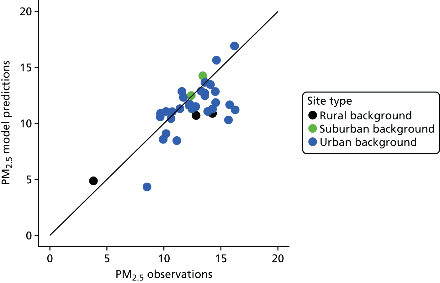
FIGURE 10.
Scatterplots of 2012 annual average modelled vs. measured PM10 concentrations (µg/m3) at GB sites.
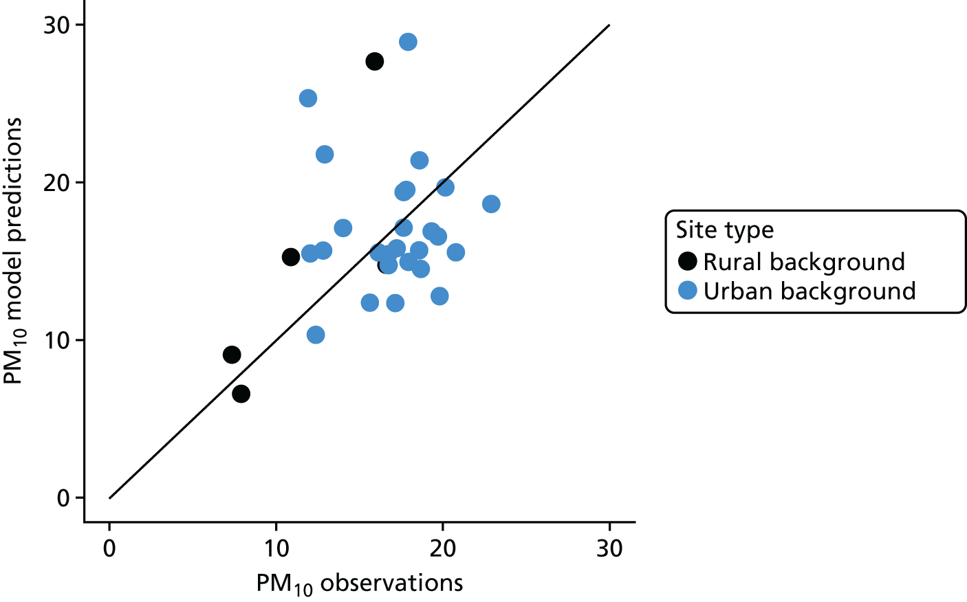
Comparison between 20-m annual average calculations of NO2 against Great Britain ambient measurements
Although dominated by sites in London, we have evaluated the CMAQ-Urban model at 20-m resolution against observations at 76 sites throughout GB in 2011; the results are summarised in Table 9 and Figures 11 and 12. In common with predictions at the background sites described above, a degree of underestimation of NOX within the emissions inventories and especially from road transport leads to underprediction of both NOX and NO2, although the NO2 mean bias is small at –5.2 µg/m3 or –11%. For both NO2 and NOX the correlation coefficient shows the model to be working well close to road sources in urban areas giving values of 0.81 and 0.75, respectively.
| Pollutant | n | Statistic | |||||||
|---|---|---|---|---|---|---|---|---|---|
| FAC2 | MB | MGE | NMB | NMGE | RMSE | r | IOA | ||
| NO2 | 76 | 1.0 | –5.2 | 8.9 | –0.11 | 0.20 | 12.4 | 0.81 | 0.71 |
| NOX | 76 | 0.8 | –34.5 | 37.7 | –0.36 | 0.39 | 56.0 | 0.75 | 0.62 |
| PM10 | 73 | 1.0 | –5.2 | 5.4 | –0.20 | 0.22 | 6.3 | 0.8 | 0.41 |
FIGURE 11.
Scatterplots of 2011 annual average modelled at 20 m vs. measured NO2 concentrations (µg/m3) at GB site.

FIGURE 12.
Scatterplots of 2011 annual average modelled at 20 m vs. measured PM10 (µg/m3) at GB sites.
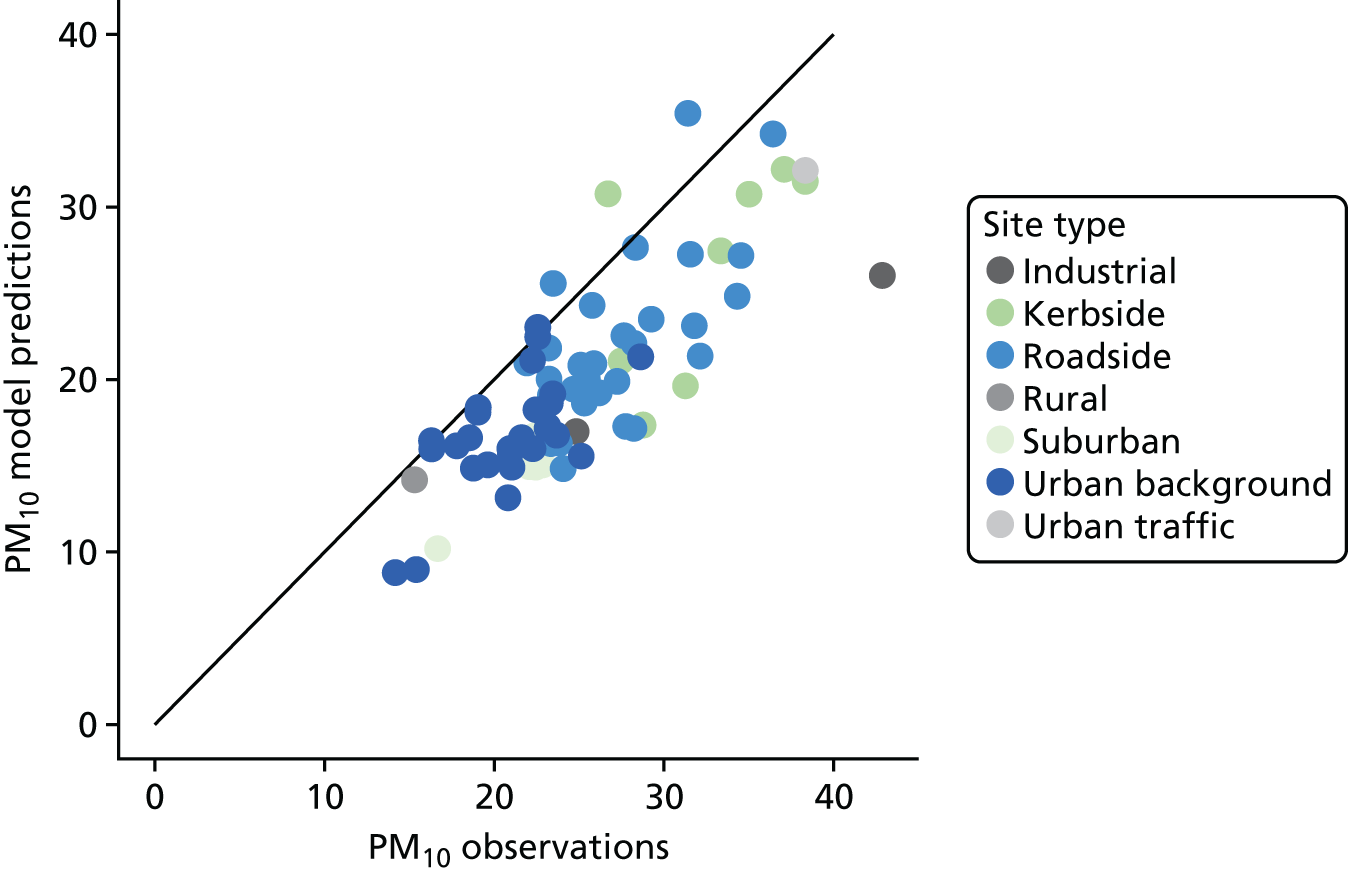
The scatterplot in Figure 11 demonstrates the close agreement between the model and observations at lower rural concentrations and an increase in divergence at higher concentrations, in which road traffic is a more important emissions source and the lack of NOX within the inventory is more influential.
Comparison of 73 sites from rural through to kerbside locations shows that the prediction of PM10 concentrations has a consistent bias of –5.2 µg/m3 or –20%, suggesting that a spatially consistent source of PM10 was missing from the model. As there is a consistent bias, the correlation coefficient between model predictions and observations is in reasonably good agreement, with an r-value of 0.8.
Hourly time series of air pollution data in Great Britain in 2012
It is also important for the model to capture the seasonal changes in air pollution concentrations as well as high air pollution ‘episodes’ during the year. To demonstrate CMAQ-Urban’s capability, we have plotted the hourly NO2 and O3 concentrations from the 10-km model (‘modelled’ time series in Figures 13 and 14) and measurements (‘observed’ time series in Figures 13 and 14) averaged across all GB sites, together with the composite frequency distribution of hourly values.
FIGURE 13.
Time series of 2012 hourly average modelled vs. measured (observed) NO2 concentrations (µg/m3) at GB sites. Mod, modelled; obs, observed.

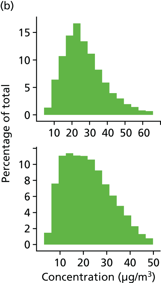
FIGURE 14.
Time series of 2012 hourly average modelled vs. measured (observed) O3 concentrations (µg/m3) at GB sites. Mod, modelled; obs, observed.

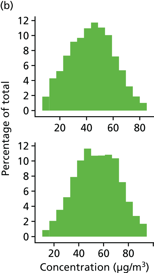
The seasonal variation of average model and measured NO2 concentrations show typical maxima during autumn and winter months and a spring/summer minimum. Most of the high episodes of NO2 are present in both time series, although they sometimes differ in magnitude (e.g. the modelled episodes in October/November are larger in magnitude than in the observed trace). Furthermore, the variability (peak to trough) of NO2 concentrations in summer is higher in the model than in the measurements. Overall, however, the hourly model results perform very well against the observations at the GB sites.
Similarly, the average modelled and measured hourly O3 concentrations show a similar seasonal profile, with a spring maximum at the end of April and autumn/winter minimum (see Figure 14), albeit with far more variability in concentrations between the largest and smallest values during this period. It is also notable that peak O3 concentrations in early January are almost as high as during the peak O3 season of April to June. Overall, the minimum–maximum range in concentrations is similar, although the modelled mean values are approximately 10 µg/m3 higher than from observations. This may also be a result of the underestimation of NOx emissions. The modelled frequency distribution is slightly skewed to higher concentrations, whereas the observed distribution is skewed towards lower concentrations, suggesting that the model overestimates lower O3 concentrations because titration of O3 with NO is reduced.
Finally, the measured and modelled average hourly time series of both PM2.5 and PM10 (Figures 15 and 16) show very good agreement throughout the year with less of a seasonal variation evident than for NO2 and O3, but a summer minimum and autumn and winter maximum, by virtue of the difference in frequency and magnitude of air pollution episodes during these periods. The mean difference in PM2.5 and PM10 is also small (approximately 1–2 µg/m3).
FIGURE 15.
Time series of 2012 hourly average modelled vs. measured (observed) PM2.5 concentrations (µg/m3) at GB sites. Mod, modelled; obs, observed.

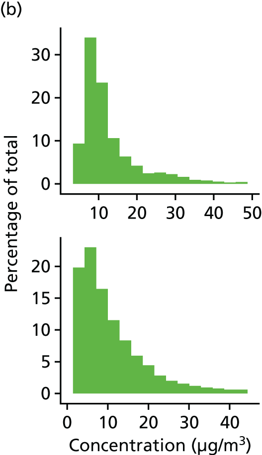
FIGURE 16.
Time series of 2012 hourly average modelled vs. measured (observed) PM10 concentrations (µg/m3) at GB sites. Mod, modelled; obs, observed.
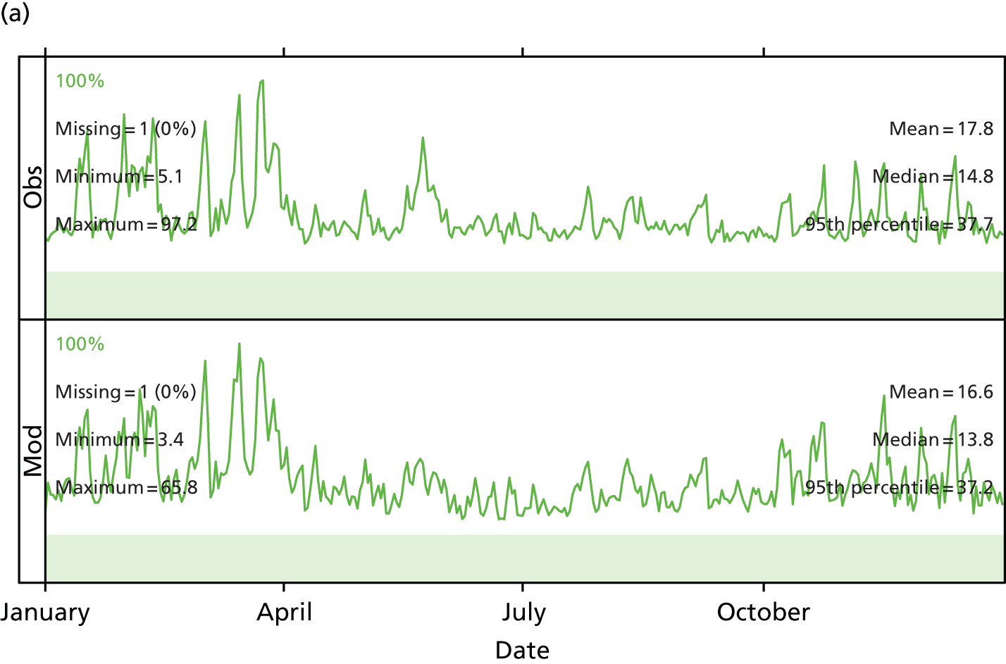
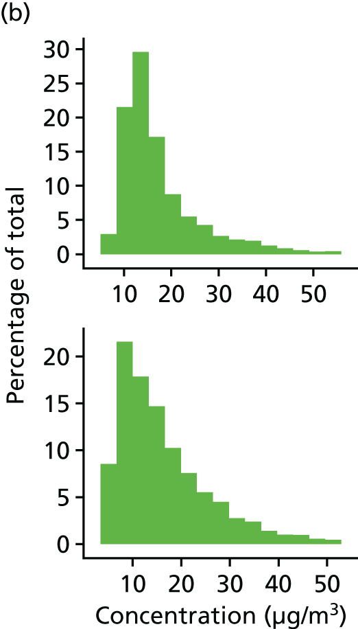
Conclusions
Model evaluation at rural, suburban and urban background sites in 2012 and from sites at locations from rural to kerbside in 2011 has demonstrated that the CMAQ-Urban model is capable of producing robust predictions of air pollution and, importantly, that this can be undertaken without the need for a ‘calibration’ of the model against measurements. This is important as models that have been ‘calibrated’ risk introducing bias into future predictions and under different policy scenarios as they assume that the same correction factor applies both now and into the future. Here we have made a determined effort to develop the model by incorporating instead new methods for predicting PM2.5/10 using the VBS scheme and a comprehensive set of new or revised emissions from diesel car IVOCs, cooking and biomass burning, as well as improved NOX and NO2 from road transport. Despite making good progress with PM predictions, which have hitherto been underpredicted, and often by a large margin, there remains room for improvement in some areas, including, but not limited to, NOX emissions from road traffic, the seasonal representation of sources in the model and the suitability of chemical boundary conditions. Nonetheless, the model is capable of producing robust projections of future air quality on which to base assessments of future policy scenarios.
Chapter 6 Current and future air pollutant concentrations
The CMAQ model, as described above, has been used to calculate ground-level concentrations at a range of spatial scales across GB. Rather than discuss all of the calculations, for clarity here we discuss just the 10-km resolution calculations for the main pollutants: PM10, PM2.5, NO2 and O3. These pollutants are chosen for discussion here as they represent the main contributors to air pollution-related health impact in GB and are also of most concern in relation to health-related guidelines and legal standards. We have also modelled at two finer spatial scales, namely 10-km grids in rural areas and 2-km grids in urban areas (10 km/2 km), and a further set of model runs at 20-m resolution in urban areas (10 km/20 m), using the CMAQ-Urban model. The 10 km/2 km resolution model runs have been used to calculate the health impact as health outcome data are not readily available at 20-m resolution. Here the intention is to give an overview of the main features of the concentration changes in the future scenarios based on the 10-km model runs. A summary of the average concentrations in GB and, for illustration, in London is shown in Table 10. The concentrations in each grid square within a ward are first averaged, then the GB and London values are averaged over all wards within those two areas. Figures and data on the other pollutants and scenarios are available on request.
| Scenario | Pollutant (µg/m) | |||||||||
|---|---|---|---|---|---|---|---|---|---|---|
| NO2 | PM2.5 | O3 (long term) | O3 (short term) | |||||||
| 10 km | 10 km/2 km | 10 km/20 m | 10 km | 10 km/2 km | 10 km/20 m | 10 km | 10 km/2 km | 10 km | 10 km/2 km | |
| London | ||||||||||
| 2011 | 26.04 | 28.36 | 30.16 | 12.79 | 13.26 | 13.35 | 32.29 | 31.55 | 91.13 | 88.91 |
| 2035 baseline | 10.66 | 11.34 | – | 6.85 | 7.17 | – | 30.17 | 29.26 | 100.90 | 99.31 |
| 2050 baseline | 15.07 | 15.61 | – | 8.05 | 8.45 | – | 27.83 | 27.38 | 97.80 | 96.38 |
| 2035 NRPO/LGHG | 13.34 | 14.64 | 14.91 | 12.59 | 13.06 | 12.90 | 29.35 | 28.27 | 99.26 | 97.32 |
| 2050 NRPO | 12.78 | 13.70 | 13.91 | 8.40 | 8.78 | 8.78 | 29.17 | 28.24 | 99.36 | 97.64 |
| 2050 LGHG | 8.61 | 8.76 | – | 8.24 | 8.61 | – | 30.15 | 29.31 | 101.71 | 100.38 |
| GB | ||||||||||
| 2011 | 12.90 | 13.75 | 13.92 | 9.35 | 9.54 | 9.54 | 35.20 | 34.92 | 96.80 | 96.26 |
| 2035 baseline | 6.31 | 6.65 | – | 4.75 | 4.85 | – | 28.65 | 28.42 | 101.33 | 100.94 |
| 2050 baseline | 10.16 | 10.79 | – | 5.73 | 5.87 | – | 26.97 | 26.82 | 98.76 | 98.38 |
| 2035 NRPO/LGHG | 6.55 | 6.97 | 6.96 | 7.31 | 7.43 | 7.41 | 28.54 | 28.29 | 101.12 | 100.67 |
| 2050 NRPO | 6.36 | 6.72 | 6.70 | 5.33 | 5.43 | 5.43 | 28.26 | 28.04 | 101.02 | 100.61 |
| 2050 LGHG | 5.21 | 5.41 | – | 5.16 | 5.26 | – | 28.28 | 28.07 | 101.58 | 101.25 |
Even when restricting the discussion to the main pollutants, there is still a potentially large number of figures that could be shown. For clarity, and to put some quantitative information on maps of concentrations, we have plotted box-and-whisker plots for each pollutant for the scenarios and mapped the concentration in each year/scenario combination. The box-and-whisker plots summarise the frequency distribution of the 10-km grid square concentrations across GB in each scenario year. In the box plots, the bottom and top of the box represent the 25th to 75th percentiles of the 10-km grid square average concentrations, the middle line in the box is median. The bars at the top and bottom of the plots are the maximum and minimum concentrations over all the grid squares. The value of the maximum is shown on each plot; the y-axis scale is relevant to all other parts of each plot. The pattern of concentrations from one scenario to another follow broadly the pattern of emissions discussed above with some important provisos. Urban concentrations tend to be influenced mainly by emissions in the residential, transport and services sectors because these emissions mainly occur in urban areas and the releases are at or near ground level. Emissions from industry and power generation tend to occur outside urban areas and the releases are generally from higher stacks. An approximate inverse power law relates emissions to release height.
It should be stressed that throughout this modelling study there has been no attempt to assess compliance with legal limit values or standards, although the model now developed at King’s College London is perfectly capable of performing such calculations.
Air quality: nitrogen dioxide
Absolute values of the annual mean concentrations of NO2 in the various scenarios are shown as box-and-whisker plots in Figure 17, and the changes relative to the base year are shown as maps in Figure 18.
FIGURE 17.
Box-and-whisker plots for annual mean GB NO2 concentrations (10-km resolution).

FIGURE 18.
Annual mean NO2 concentrations in the various scenarios. (a) 2011; (b) 2035 baseline; (c) 2050 baseline; (d) 2035 NRPO; (e) 2050 NRPO; and (f) 2050 LGHG.
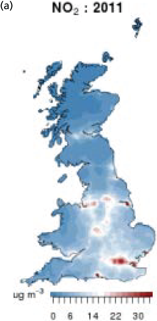

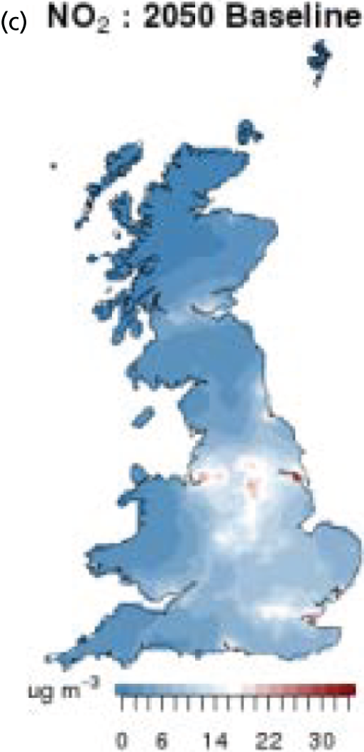
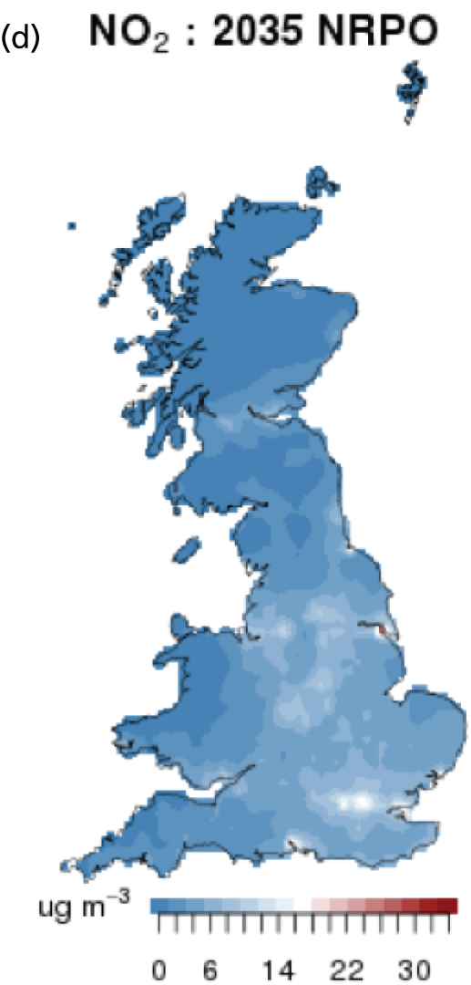

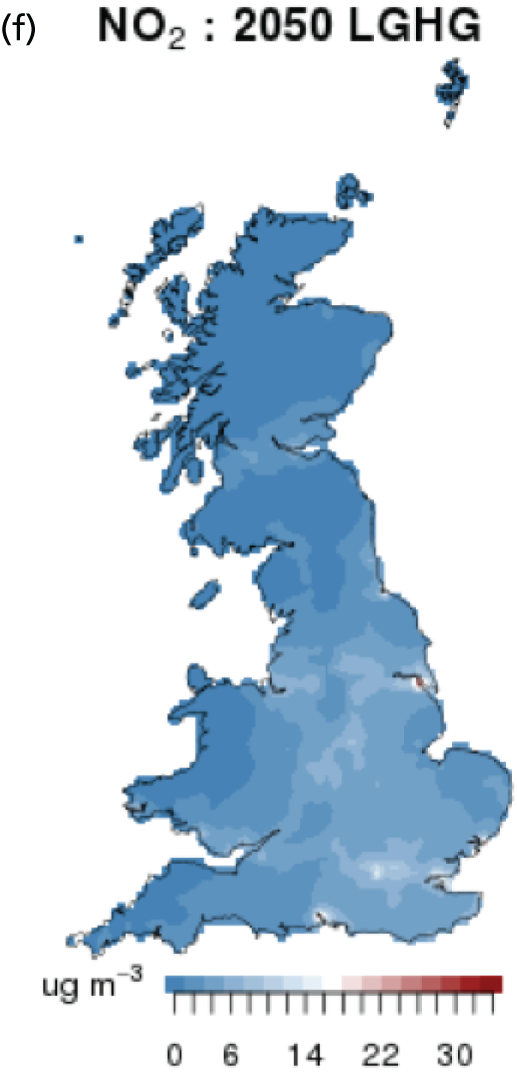
Almost all the scenarios show significant decreases in annual mean NO2 concentrations, largely as a result of the electrification of large parts of the road transport sector. The one exception is the baseline scenario. Here, there was no obligation to meet the CCA target, nor was there any carbon price imposed in the model. This resulted in a higher consumption of natural gas (notably in the industrial sector) and oil products (in the transport sector) in 2050 (compared with the LGHG scenario), leading to a much smaller reduction in NOX concentrations in 2050 than in the other scenarios. The decreases in all scenarios are largely a consequence of the electrification of the vehicle fleet: the LGHG and the NRPO scenarios have very similar levels of car fleet electrification, but the NRPO scenario has more gas consumption in stationary sources leading to smaller reductions in NO2 overall compared with the LGHG scenario. The LGHG scenario shows the largest decrease in NO2 concentrations in 2050, with the highest level of nuclear energy and the smallest use of oil and gas in meeting the CCA target, although by 2050 the reductions in the NRPO scenario are similar. Annual mean concentrations of NO2 in these scenarios are projected to decrease by more than ≈50% in the highest 25% of 10-km grid squares in GB. The scenario, which does not meet the CCA target, shows the smallest decreases in NO2. These are important conclusions given the current interest in NO2 levels and the legal limits in the legislation.
The hourly results for all GB sites for NO2 are shown in Figure 19. The effect of the electrification in the road transport sector is clearly apparent in the frequency distributions.
FIGURE 19.
Hourly NO2 concentrations at all GB sites in the different scenarios.
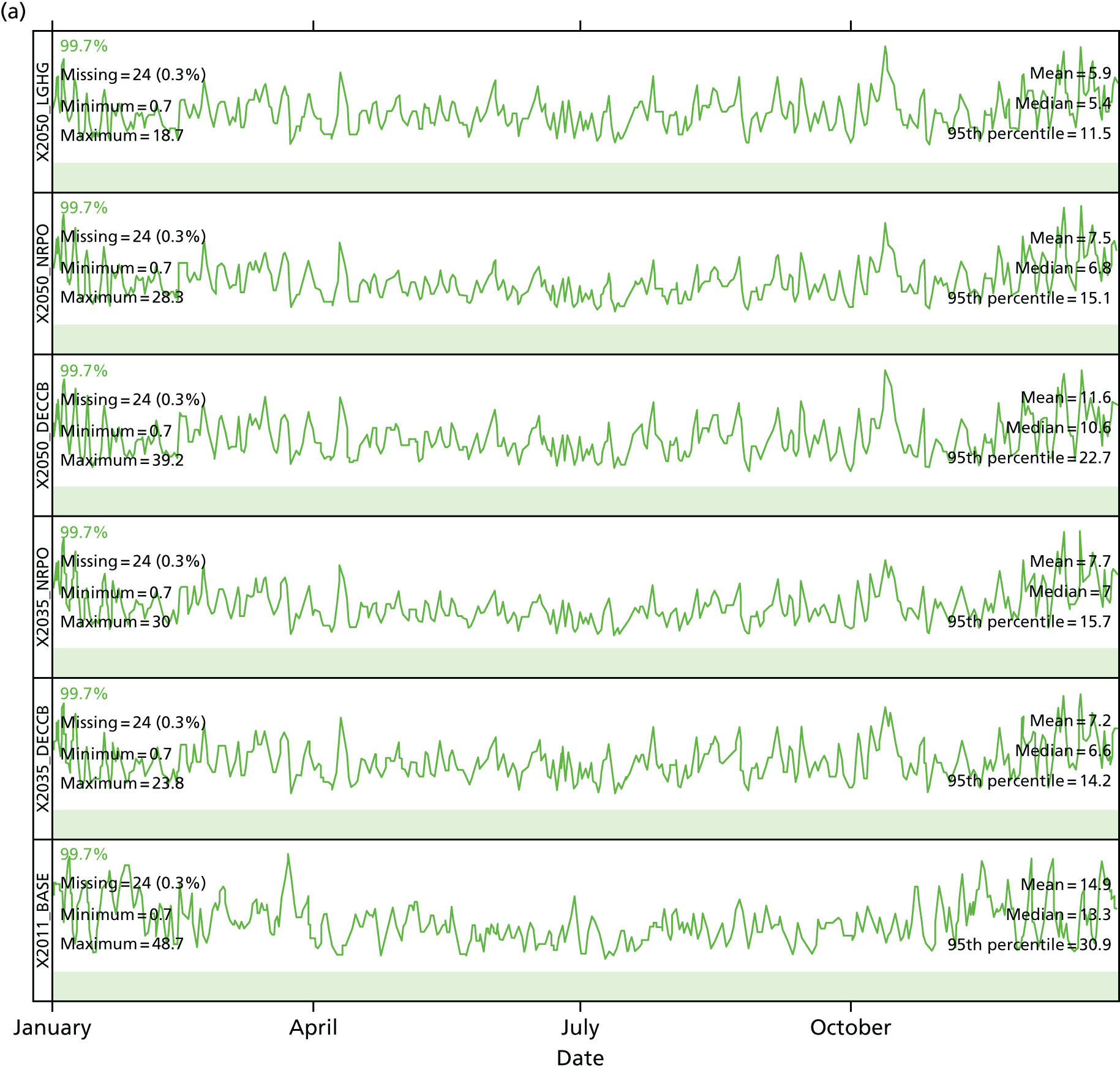
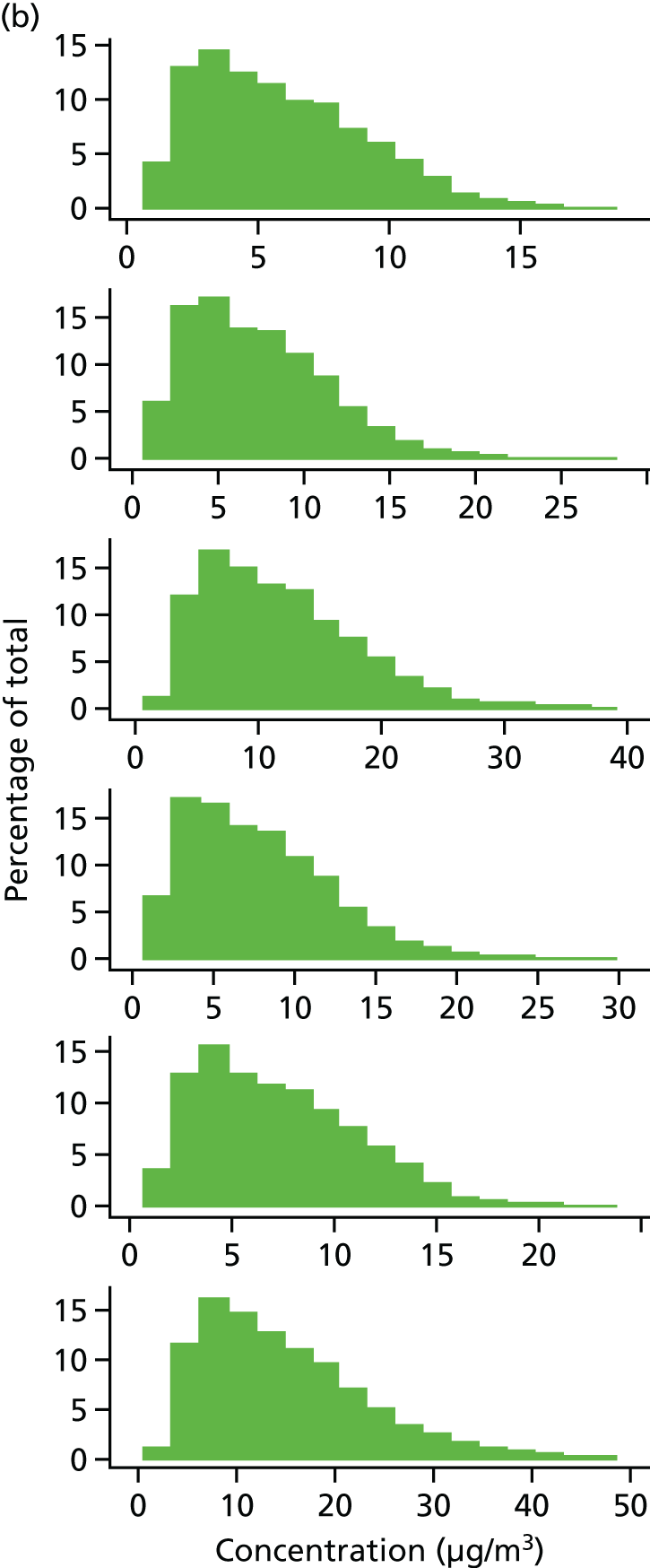
Even the baseline scenario, which does not meet the CCA target, shows a large decrease in hourly peak concentrations, but the NRPO and LGHG scenarios show even larger reductions.
Figures 20 and 21 show the time series for the base year 2011 and the NRPO showing even more clearly the reduction in hourly concentrations of NO2 in the future as the road transport fleet becomes electrified.
FIGURE 20.
Hourly concentrations of NO2 across all GB sites in the base year and NRPO scenarios.

FIGURE 21.
Hourly concentrations of NO2 at the London North Kensington site in the base year (2011) and the NRPO scenario.
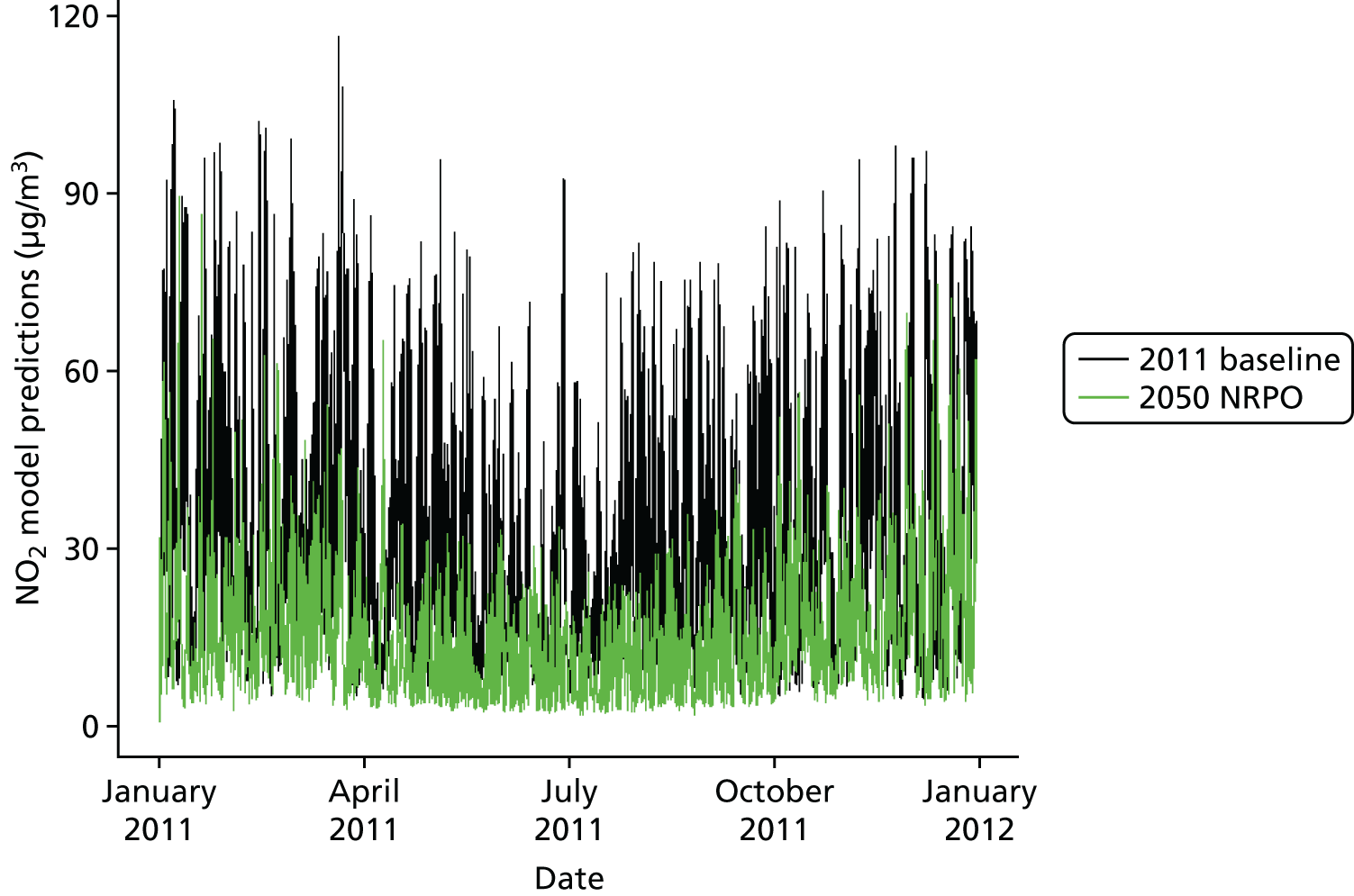
Air quality: PM2.5
Similar plots are shown for annual mean PM2.5 in Figures 22 and 23.
FIGURE 22.
Box-and-whisker plots of annual PM2.5 concentrations in the different scenarios.
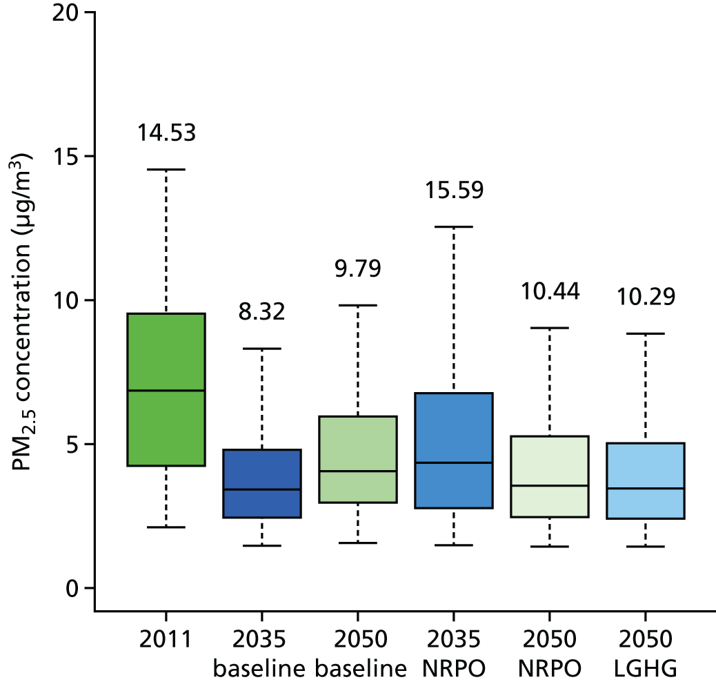
FIGURE 23.
Annual mean PM2.5 concentrations in the various scenarios. (a) 2011; (b) 2035 baseline; (c) 2050 baseline; (d) 2035 NRPO; (e) 2050 NRPO; and (f) 2050 LGHG.
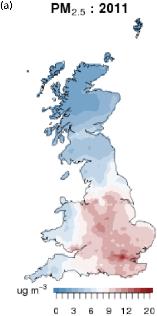
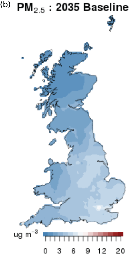

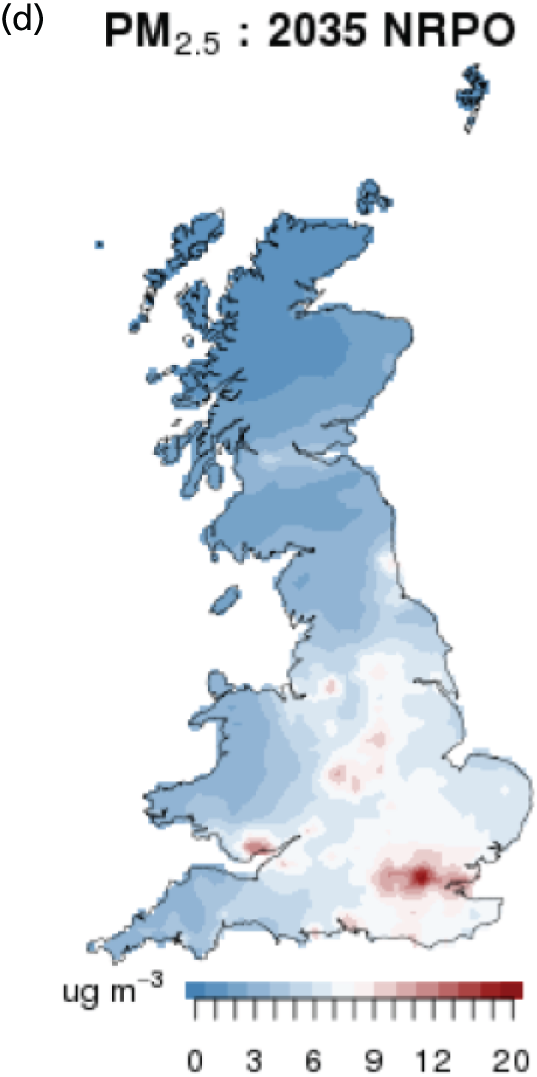
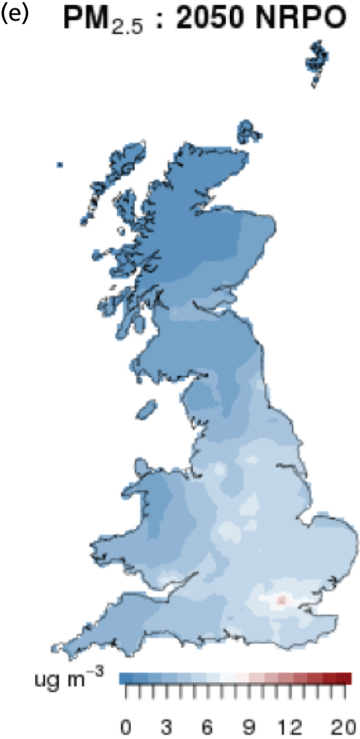
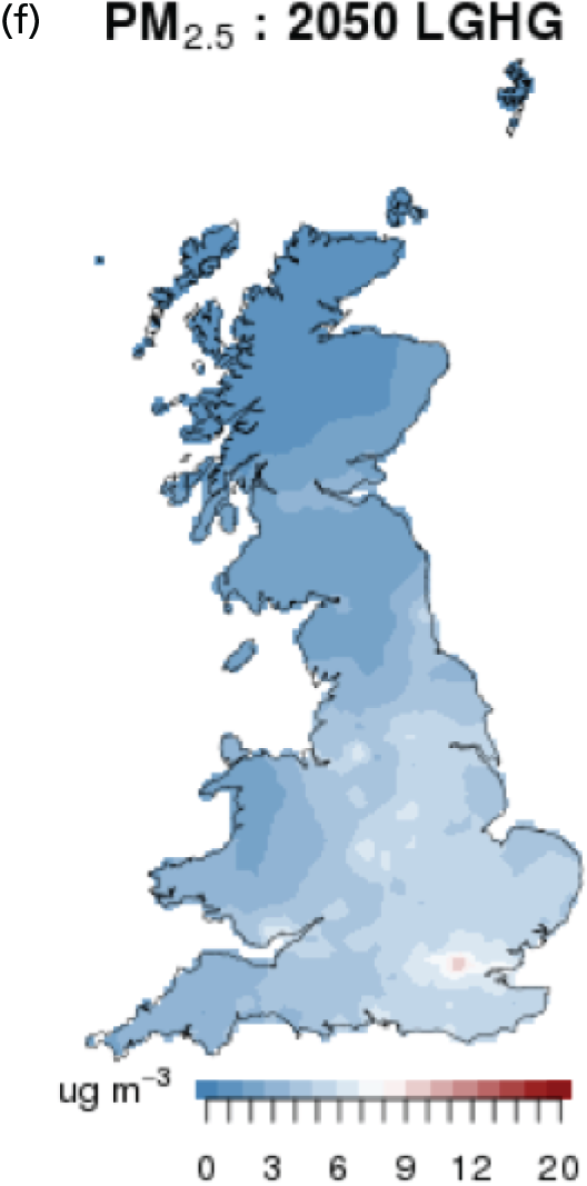
It is clear from these plots that, overall, total PM2.5 concentrations are projected to decrease relative to 2011 in all scenarios. However, this overall behaviour masks potentially important issues. The reductions in total PM2.5 concentrations are influenced strongly by the secondary aerosol components of ammonium sulphate and nitrate, which are projected to decrease significantly out to 2050 largely because of reductions in NOx and SO2 emissions arising from GB and the rest of Europe. These reductions outweigh the changes in primary PM2.5 emissions. Reductions in traffic exhaust primary PM2.5 emissions are projected to occur as a result of increasing use of diesel particle filters in Euro 6 and IV vehicles in the earlier years and the increasing electrification of the road transport fleet further out to 2050. However, within this broad behaviour, projections from UKTM show increased use of biomass use at a similar scale in both the LGHG and the NRPO scenarios. This use is projected to peak in 2035 in the NRPO scenario with a consumption of 1126 PJ compared with only 292 PJ in 2010. By 2050 the biomass use has only decreased slightly from the 2035 peak to 932 PJ in the NRPO scenario. This means that, on this basis, although the median total PM2.5 concentrations across the country are projected to decrease in 2035, in some areas, notably London, South Wales and the North East, total PM2.5 concentrations are projected to increase. The same behaviour is likely to be true for the LGHG scenario, although the plots for this scenario are not shown here. The baseline scenario does not show this increase in biomass use, but this is because the scenario does not have the CCA target as a constraint, nor does it have a carbon price included. By 2050, total PM2.5 levels are projected to decrease in all scenarios with smaller reductions in absolute levels (but not necessarily percentage reductions) occurring in Scotland, where existing levels are overall lower than in the rest of the country.
The increase in primary PM2.5 is more clearly demonstrated in Figures 24 and 25, in which we have plotted the sum of elemental carbon (EC) and OA, as this sum is a good approximation of the primary PM2.5 concentration.
FIGURE 24.
Box-and-whisker plots for annual mean EC + OA.

FIGURE 25.
Annual mean EC + OA in the various scenarios. (a) 2011; (b) 2035 baseline; (c) 2050 baseline; (d) 2050 LGHG; (e) 2035 NRPO; and (f) 2050 NRPO.
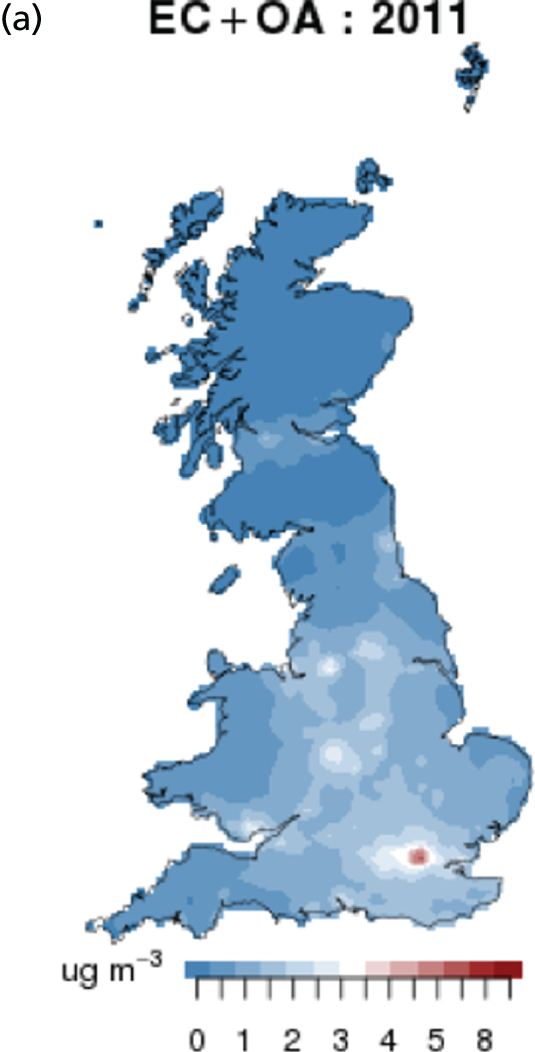
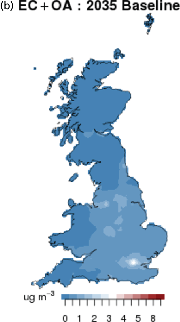
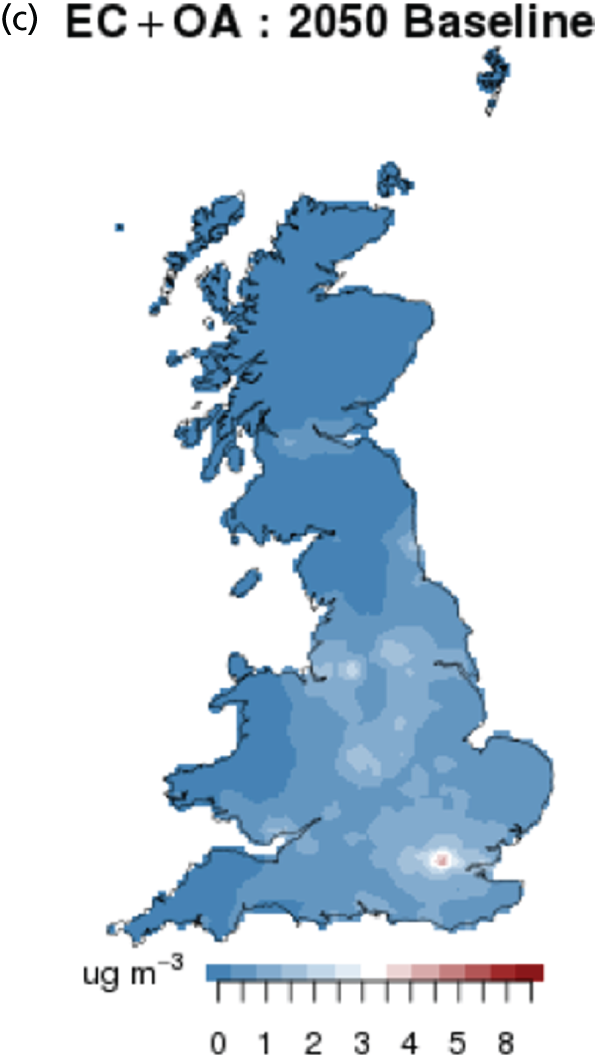
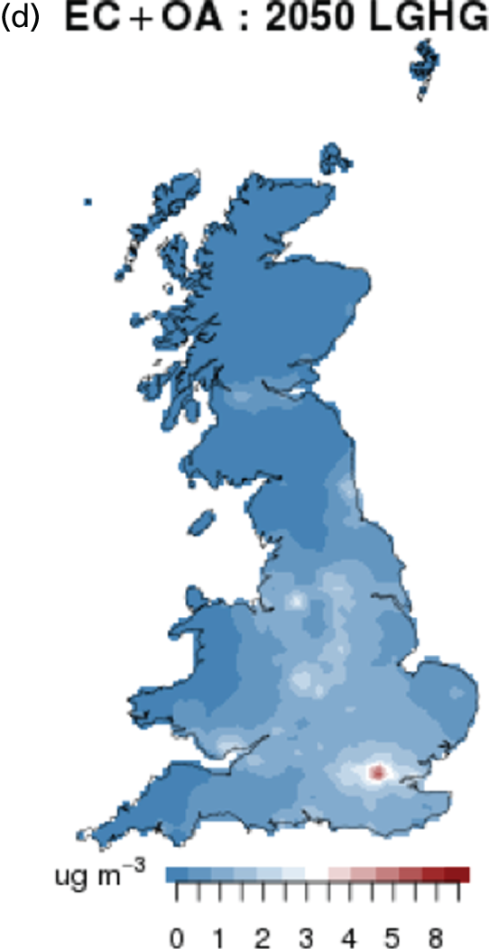
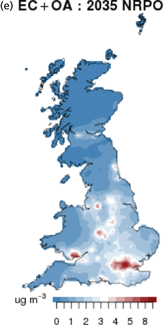

It is clear from these plots that the NRPO scenario, with the large increase in biomass use, shows a large relative increase in EC and OA in the period out to 2035; the LGHG scenario will show the same behaviour. Within the health effects community there is, at present, no consensus on the relative toxicity of the various components of PM2.5 (or of PM10) so the precise health implications of this increase are unclear. However, there is a body of evidence linking black carbon (essentially the same component as EC + OA) with adverse health effects (and these emissions are likely to contain carcinogens). 93 As noted above, the biomass use peaks in 2035 but decreases further by only a relatively small amount by 2050. By that year, the median level of EC and OA in the LGHG and NRPO scenarios has decreased by a small amount, but the outliers at high concentration remain as high as they were in 2011.
Overall, therefore, although both scenarios that meet the CCA target show decreases in total annual mean PM2.5 levels by 2050, both scenarios have an increase in biomass use, which prevents a more accelerated reduction in total PM2.5 and which actually leads to an increase in concentrations of primary PM2.5 components in 2035 with a relatively small reduction in 2050 compared with 2011 levels.
Annual mean PM2.5 concentrations in the LGHG and NRPO scenarios are projected to fall by around 40% in the top 25% of grid squares, but by only ≈25% in the highest areas. However, the concentrations of EC and OA are projected to increase in 2035 in the NRPO and LGHG scenarios by around 30–60% in the more polluted grid squares. By 2050, in those two scenarios, levels are only slightly smaller than 2011 values and in the highest grid square very similar to 2011 concentrations. If this amount of primary PM2.5 were to be removed, by avoiding the use of biomass as indicated in the NRPO and LGHG scenarios, the total PM2.5 concentrations could fall even further than projected, potentially down by ≈50% in the highest areas compared with a ≈25% reduction with the increased biomass use.
Air quality: PM10
Similar plots for PM10 are shown in Figures 26 and 27.
FIGURE 26.
Box-and-whisker plots for annual mean PM10 concentrations in the various scenarios.
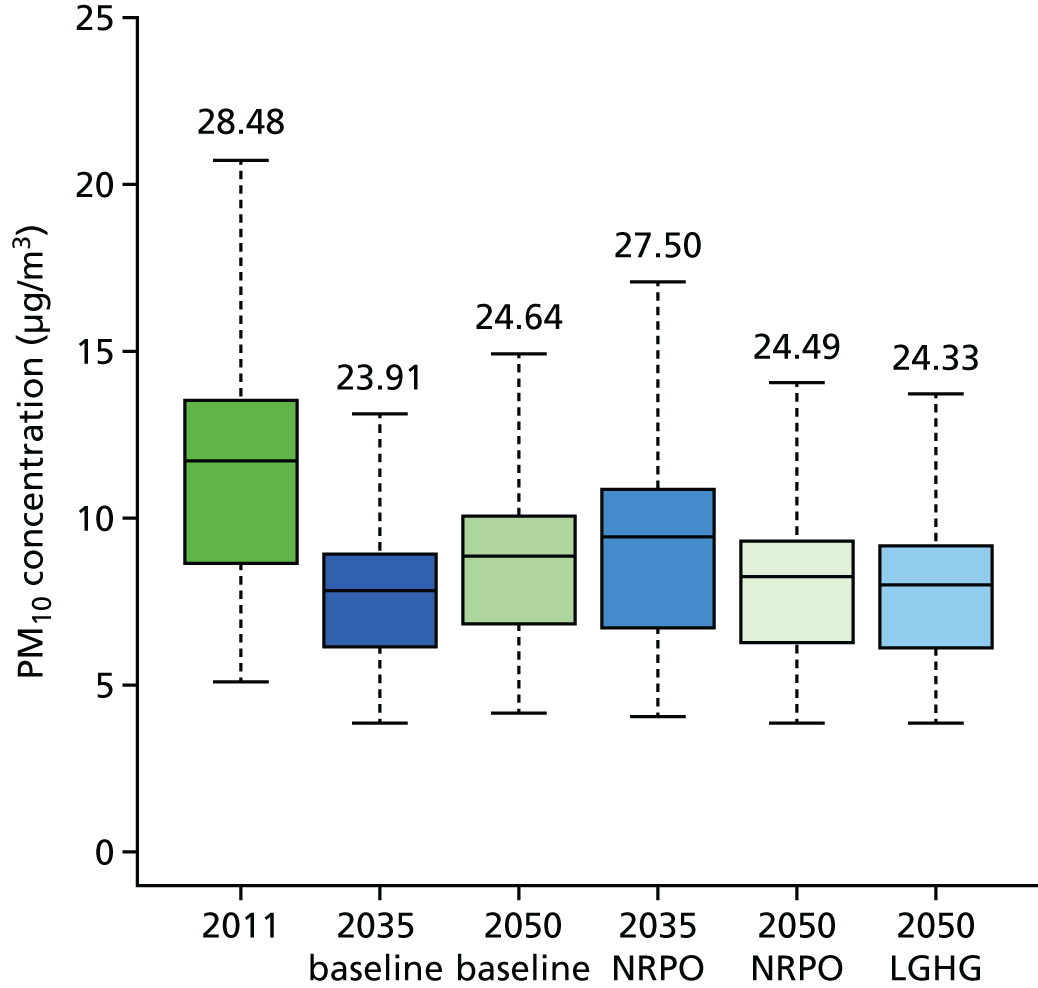
FIGURE 27.
Annual mean PM10 concentrations in the various scenarios. (a) 2011; (b) 2035 baseline; (c) 2050 baseline; (d) 2035 NRPO; (e) 2050 NRPO; and (f) 2050 LGHG.


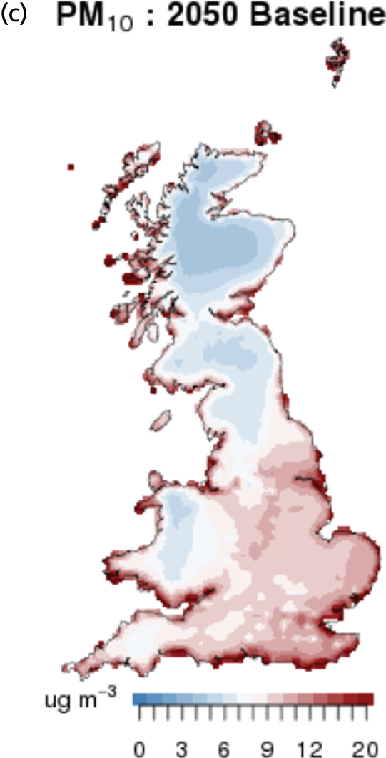
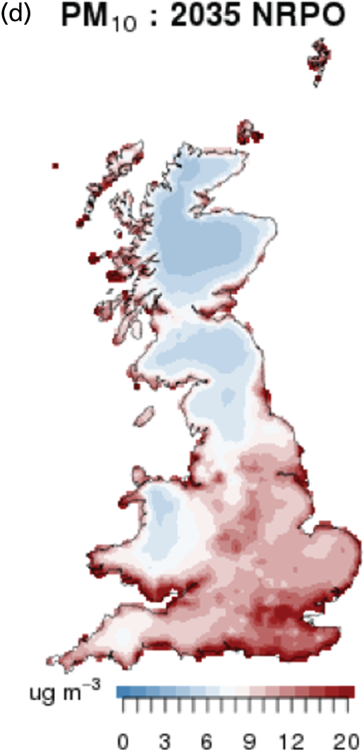
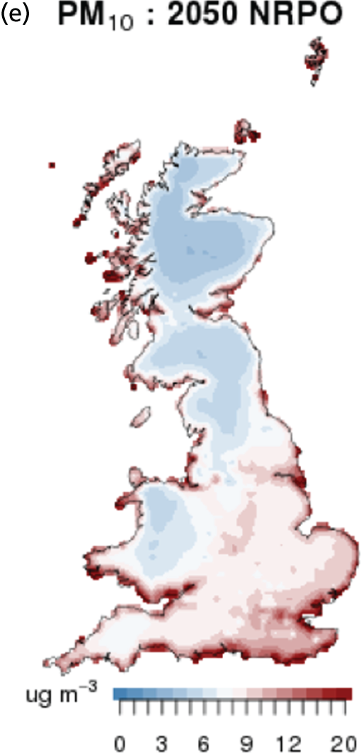

The comments regarding biomass use in Air quality: PM2.5 also apply to PM10. Moreover, an additional component of PM10 emissions is important here, namely non-exhaust emissions from brake, tyre and clutch wear and resuspended road dust. Emissions from this source are uncertain and further research is needed to make more accurate estimates. However, based on current knowledge, these emissions already make up the largest part of emissions of primary PM10 from the road transport sector. In 2014, non-exhaust emissions from road transport in the UK were 73% of the total road transport PM10 emissions. By 2050 the PM10 emission factors from non-exhaust sources are assumed to be the same as they are now, as discussed above. On this basis, the total road transport PM10 emissions in the NRPO scenario are projected to increase by about 15% from 2011 to 2050 as a result of the projected increase in vehicle kilometres driven over that period. This increase in non-exhaust emissions by 2050 will also affect PM2.5 concentrations, although to a lesser extent than PM10 (in 2050 the road transport emissions of PM2.5 are about 27% of those of PM10).
The consequence of this is that, despite the reduction in secondary PM10 concentrations resulting from the decreases in NOx and SO2 emissions in GB and the rest of Europe, PM10 concentrations are projected to increase in 2035 in the NRPO (and LGHG) scenario in many areas of GB, despite the median concentration showing a decrease. By 2050 there is projected to be a small decrease in much of England but increases in western areas, Wales and Scotland, partly influenced by sea salt contributions in coastal areas.
The projected increase in non-exhaust emissions is clearly of potential concern as regards compliance with standards and guidelines. It is also of concern regarding adverse effects on public health. Research in this area is still relatively new, but there are already grounds for concern over the toxicity of non-exhaust emissions, as outlined in a recent review. 94
Air quality: ozone
Ozone is unique in the set of pollutants discussed in this report, in that different metrics behave differently in response to mitigation measures, because the different metrics are determined by different processes, unlike a less reactive pollutant, concentrations of which are generally proportional to emissions. In the case of O3, peak hourly concentrations are determined by the well-known photochemical ‘smog’ reactions involving emissions of NOx and VOCs on a regional scale. This overall process is strongly non-linear, but, in many of the more polluted areas in GB and Europe, peak O3 concentrations have up until now been more responsive to reductions in VOC emissions. Longer-term average concentrations, however, tend to behave differently, mainly because the photochemical episodes which determine the peak O3 levels occur on only a small number of occasions, at least at more temperate northern European latitudes such as GB. In the case of these longer-term annual or summer-time averages, the O3 concentration is governed by the photostationary state equations involving NO, NO2 and O3. These essentially ‘titrate’ O3 via reaction with NO:
The NO2 photolyses in sunlight to reform NO plus an oxygen atom, which re-forms O3 by reacting with an oxygen molecule:
These reactions take place very quickly (in minutes) during sunlight and thus interchange O3 and NO2 very quickly, such that the sum O3 + NO2, defined as oxidant (Ox), is conserved. The important point for long-term average O3 concentrations is that as NOx concentrations decrease, the titration reaction removes less O3 and average O3 levels increase.
The health impact of O3 is discussed in more detail in the next section of the report, but here we describe the behaviour of two health-relevant concentration metrics in response to the emission reductions in the future scenarios.
The two metrics refer to long- and short-term exposures and are based on 8-hour averages, an averaging time originally determined by chamber exposure studies as providing the most relevant averaging period. The long-term exposure metric was published by WHO in its project Health Risks of Air Pollution in Europe (HRAPIE)95 and refers to the April–September average of the daily maximum 8-hour mean above 35 p.p.b. (equivalent to 70 µg/m3). The short-term metric we use here derives from the recommendation of COMEAP in its report on the quantification of the health effects of O3 96 and is the annual average of the daily maximum 8-hour mean with no threshold or cut-off point, unlike the long-term metric. This point is important in determining the response of the metric to emission reductions.
The plots of the long-term exposure metric are shown in Figures 28 and 29 for all scenarios for GB, modelled at 10-km resolution, and for London, modelled at 2-km resolution, respectively.
FIGURE 28.
Box-and-whisker plots of April–September mean of daily maximum 8-hour O3 concentrations over GB in the various scenarios (the long-term O3 exposure metric).
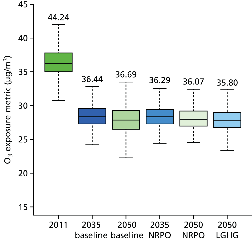
FIGURE 29.
The long-term O3 exposure metric for London in the various scenarios.
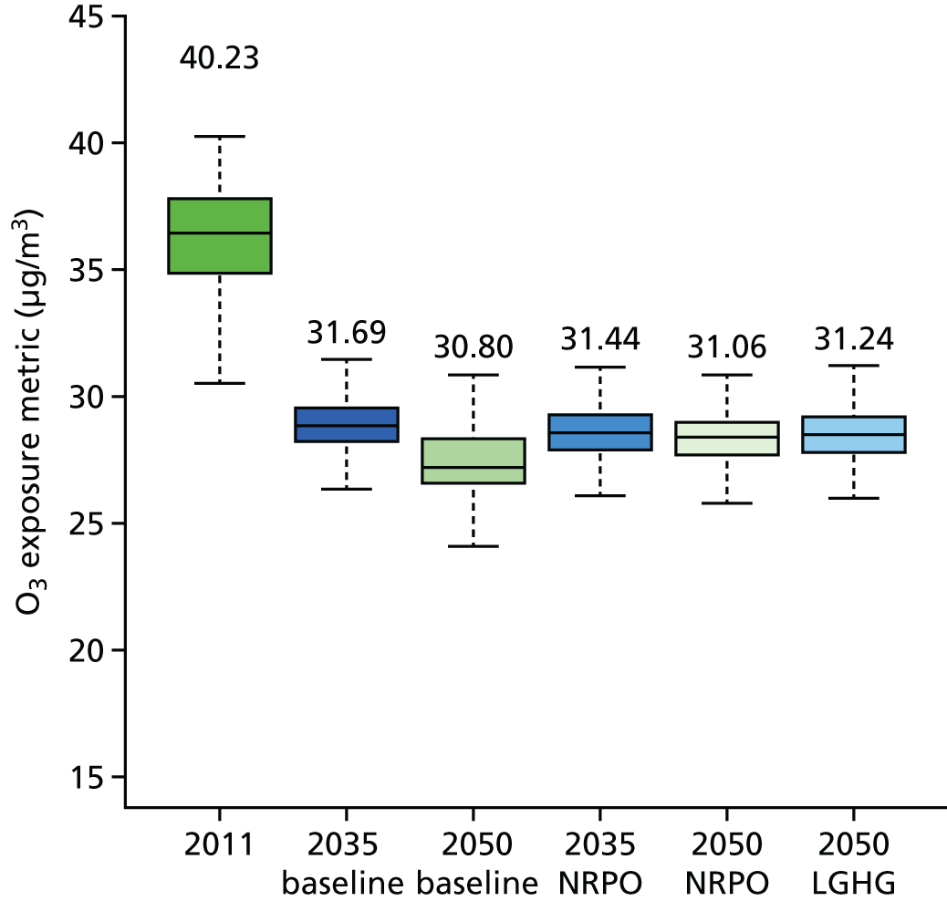
Before discussing these results it is instructive to compare the results for the short-term metric shown in Figures 30 and 31.
FIGURE 30.
Box-and-whisker plots of the annual mean of the daily maximum 8-hour O3 concentration for GB (the short-term O3 metric) in the various scenarios.

FIGURE 31.
The short-term O3 exposure metric for London.
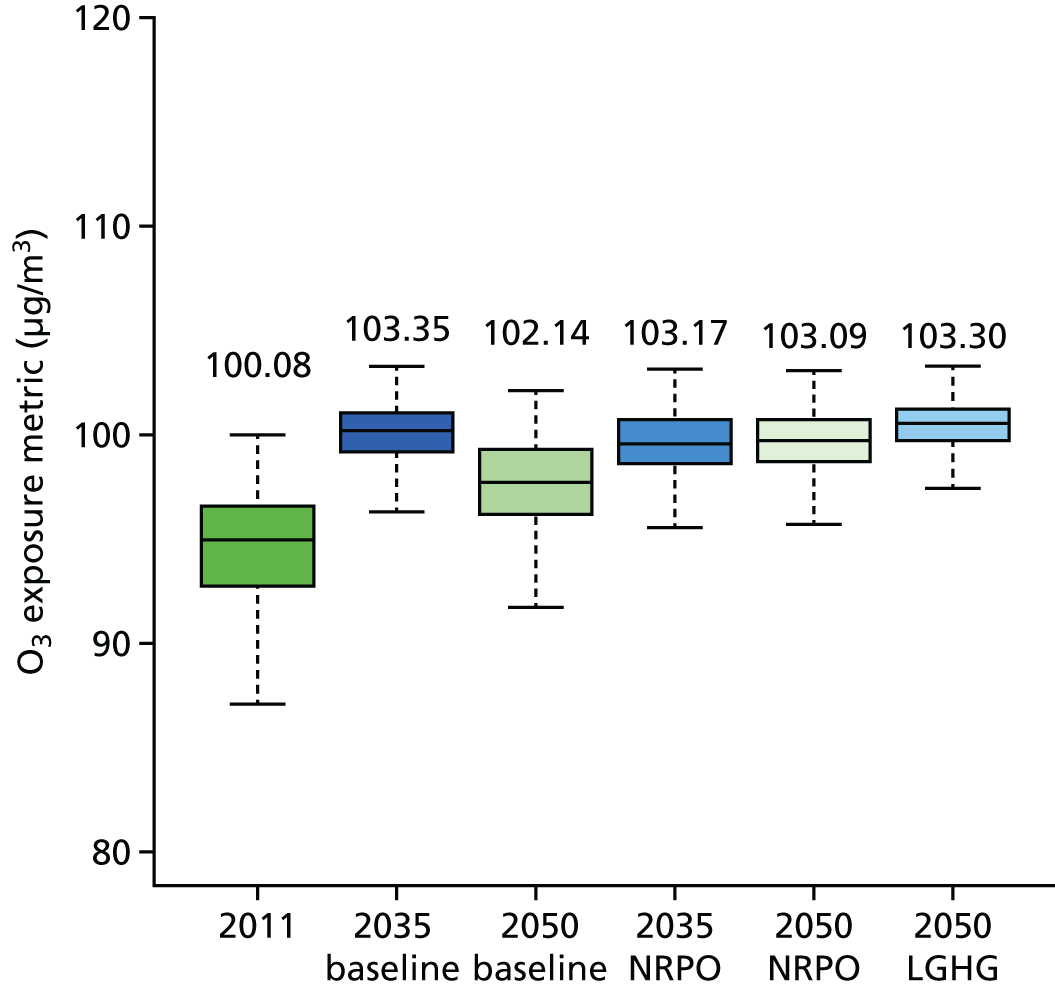
There are three main processes contributing to O3 levels in the UK. The global tropospheric background provides a baseline of around about 70 µg/m3 everywhere in GB. Superimposed on this level are summer-time O3 ‘smog’ episodes when hourly peaks can reach higher levels, typically up to ≈200 µg/m3 in the worst episodes. The third main mechanism is the so-called ‘titration’, referred to above, whereby fresh emissions of NOx can destroy O3. Combinations of these three mechanisms allow interpretation of the results in Figures 28–31. It is worth noting here that the global background O3 concentration in our modelling increased slightly in future years. This level will be dependent on global emissions of methane and of NOx and, in the scenario we have used from the ECLIPSE projections, the tropospheric baseline is projected to increase, which is the main influence on the increase of O3 annual means in GB in our model. Although we have used one set of projections for these emissions, the scope of this research does not allow us to investigate the sensitivities of GB long-term mean O3 concentrations to variations in emissions of O3 precursors in different global scenarios.
It is clear from Figures 28 and 29 that the long-term O3 exposure metric decreases in response to emission reductions in all scenarios across GB, including in the urban areas shown. This metric is calculated over the summer months, so the reductions are probably because of the reduction in VOC emissions, leading to less photochemical production of O3.
The short-term metric, however, applies over the whole year, which includes the winter months, when NOx concentrations are highest and when photochemical production from VOCs is virtually absent. This metric increases, unlike the metric for long-term exposure. The reason is that the short-term metric covers the winter months as well as the summer months and, most importantly, incorporates no threshold, so the average includes the very low O3 concentrations. These concentrations increase as NOx emissions are decreased in the future years and this mechanism clearly dominates, leading to an increase in the metric, suggesting that health-relevant short-term exposures will increase. The net effect of these two competing responses to emission reductions is not immediately clear and will be discussed in the next section of the report dealing with health impact (see Air quality: oxidant).
Hourly concentrations of O3 in the various scenarios are shown in Figures 32 and 33. The effect of the scenarios on peak hourly O3 concentrations is relatively small, although each scenario shows a maximum hourly mean higher than the maximum in the base year of 2011, with values increasing from ≈138 to ≈170–174 µg/m3. The main difference is shown by an inspection of the frequency distributions which shows clearly the increased proportion of lower O3 concentrations in the future scenarios caused by the reduction on NOx emissions. This is also the reason why the mean O3 concentration increases in future scenarios.
FIGURE 32.
Hourly O3 concentrations over all GB sites in the various scenarios.
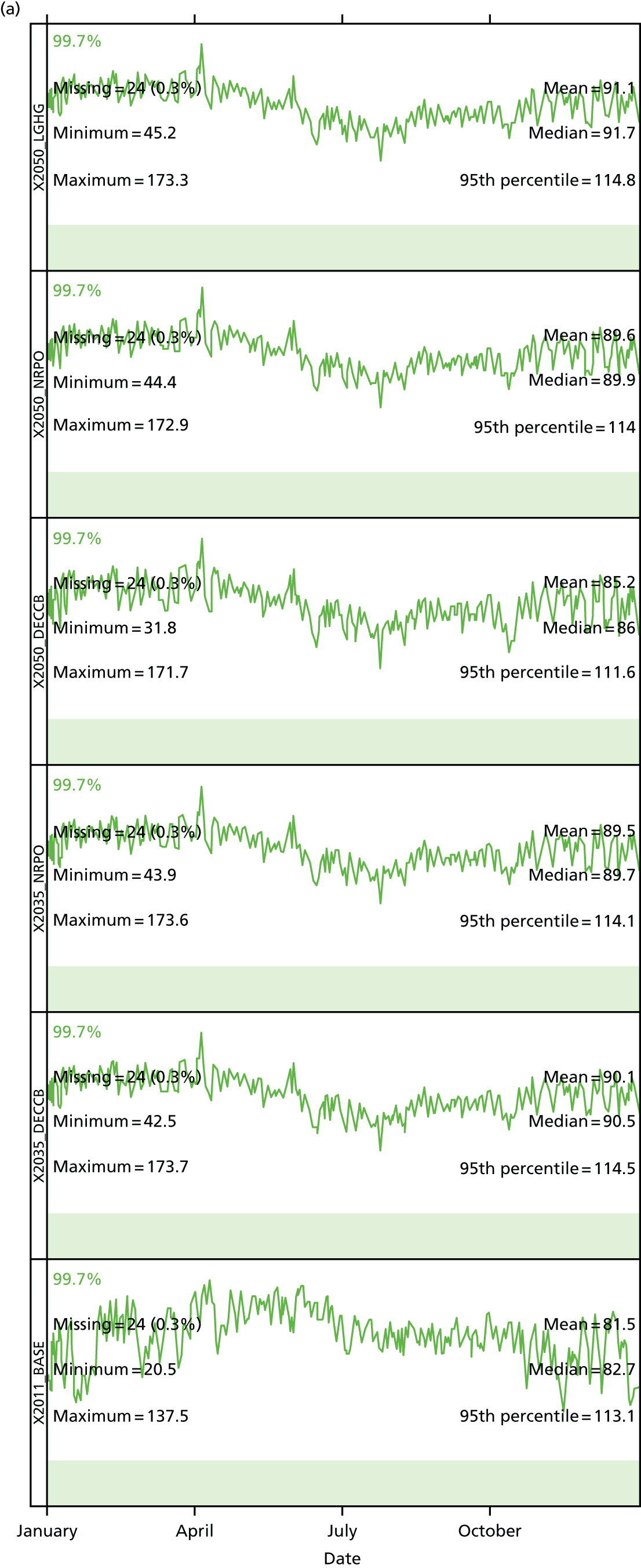

FIGURE 33.
Hourly O3 concentrations across all GB sites in the base year (2011) and the LGHG scenario.

The role of the various mechanisms in determining hourly O3 concentrations is very clearly shown in Figure 33. Here, the increase in O3 concentrations in the winter months is very clear, caused by the reduction in NOx emissions reducing the extent of O3 ‘titration’. The reduction in the summer months is probably the result of the reduction in VOC emissions in GB and the rest of Europe leading to a reduction in photochemical formation of O3.
Air quality: oxidant
It was noted in the previous section (see Air quality: ozone) that in the absence of photochemical episodes, and, hence, in terms of longer-term average concentrations, the sum of O3 plus NO2 is conserved as the two pollutants interchange rapidly in sunlight, and, as NOx concentrations reduce, O3 concentrations increase to approach the rural or tropospheric background. As well as atmospheric chemistry reasons for investigating O3 and NO2 together, there are also health reasons, as both are Ox and have the potential to cause harmful effects in humans. Literature has begun to emerge linking Ox with adverse health effects,97 so it is pertinent to investigate the effect of the energy scenarios here on future concentrations of Ox in GB.
Figures 34 and 35 show the box-and-whisker plots and the annual average Ox concentrations in the various scenarios, from which it can be seen that Ox levels change very little in the different scenarios, with an indication of a slight increase in future years compared with 2011 values. The oxidising power of the atmosphere in the future scenarios will depend on the balance between O3 and NO2 at any given point in space or time, as the two pollutants have different redox potentials. 97 In future, as NO2 concentrations decrease and annual average O3 and Ox concentrations are projected to increase, the proportions of O3 and NO2 making up Ox will shift in favour of O3. Ozone has a higher redox potential than NO2,97 so the oxidising power of the atmosphere, in terms of long-term average exposures, is projected to increase.
FIGURE 34.
Box-and-whisker plots of Ox concentrations in the various scenarios.
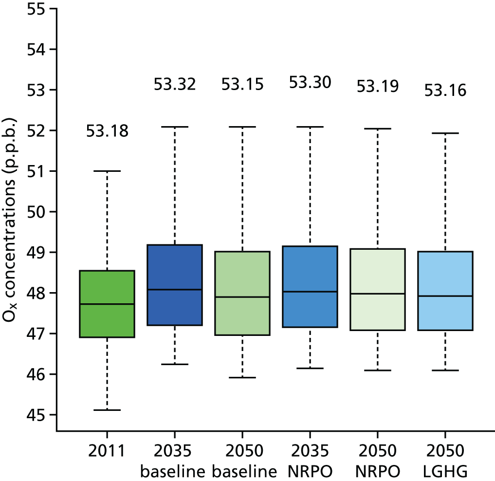
FIGURE 35.
Annual mean Ox concentrations in the various scenarios. (a) 2011; (b) 2035 baseline; (c) 2050 baseline; (d) 2035 NRPO; (e) 2050 NRPO; and (f) 2050 LGHG.

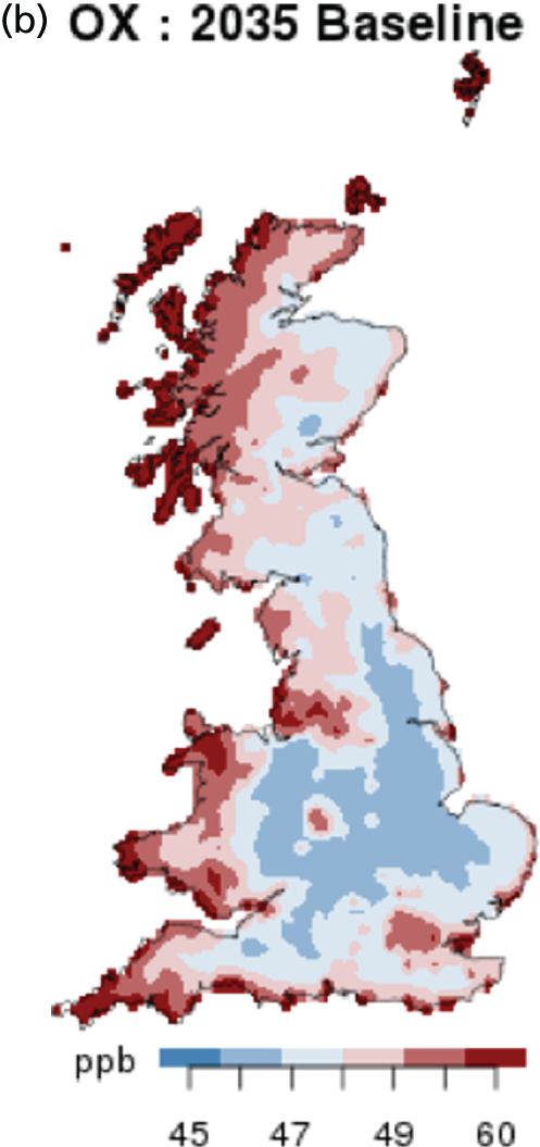
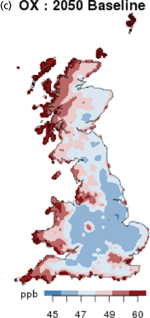
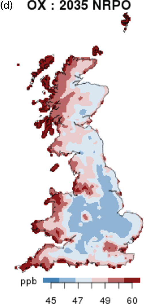

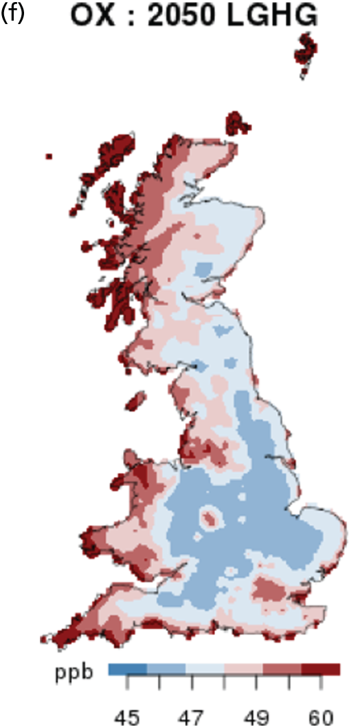
Chapter 7 Public health impact
Introductory remarks, health outcomes, concentration–response functions and methodology
It is now well established that adverse health effects, including mortality, are statistically associated with outdoor ambient concentrations of air pollutants. Moreover, toxicological studies of potential mechanisms of damage have added to the statistical evidence, such that many organisations (e.g. US Environmental Protection Agency, WHO, COMEAP) consider the evidence strong enough to infer a causal relationship between the adverse health effects and the air pollution concentrations. 98 The evidence is strongest for PM2.5, and the impact on mortality in GB of PM2.5 concentrations in 2008 were estimated by COMEAP as approximately 29,000 deaths and typically a loss of 340,000 life-years; alternatively, COMEAP suggested that this could be expressed as a 6-month loss of life expectancy from birth. 99
In the Review of the Health Aspects of Air Pollution project,93 WHO systematically examined peer-reviewed articles on air pollution and health and concluded that the evidence for the adverse effects of PM2.5 had strengthened. Significantly, this review also concluded that the evidence had now strengthened for adverse effects of NO2 independent of those from PM mass, chiefly from the use of two pollutant models in epidemiological studies. Previous assessments had concluded that it was not possible to separate the effects of PM (or other particle metrics such as ultrafine particles) and NO2, as they are highly correlated in most urban areas. The review further discussed the emerging evidence for adverse effects of long-term exposures to O3.
This section uses this epidemiological evidence to estimate the health impact of the changes in air pollutant concentrations predicted by the policy scenarios discussed in Chapter 6.
Concentration–response functions
In general, we based the CRFs on COMEAP recommendations, with the addition of WHO recommendations where these were more recent and/or provided alternative approaches.
Subsequent to the Review of the Health Aspects of Air Pollution project, WHO also reviewed the literature to produce a series of CRFs, relating the outdoor concentrations of a given air pollutant to a specific adverse health outcome,95 in the HRAPIE project. In addition to PM2.5, the HRAPIE study also recommended CRFs for all-cause mortality for long-term exposures to NO2 and to long-term (warm season) O3.
In the UK, since the HRAPIE work,95 COMEAP has separately addressed O396 and NO2100 and made recommendations for CRFs to be used in quantifying their impact. The COMEAP report, however, did not recommend a CRF for longer-term exposures to O3, considering the evidence insufficient to do so at that time.
In considering all the available assessments, we have used the CRFs in relation to long-term exposures to different pollutants and all-cause mortality (unless otherwise stated) (Table 11). The full list of studies used to derive the CRFs is given in the referenced reports.
| Pollutant | Averaging time | RR (hazard ratio) per 10 µg/m3 | Confidence interval | Counterfactual | Comment/source |
|---|---|---|---|---|---|
| PM2.5 | Annual average | 1.06 | 1.04 to 1.083 (WHO) | Aged ≥ 30 years95 | |
| 1.06 | Plausibility interval from expert judgement: 1.01 to 1.12 (COMEAP) | Aged ≥ 30 years, anthropogenic PM2.5 99 | |||
| NO2 | Annual average | 1.017 | 1.007 to 1.027 | 0 or 5 µg/m3 | Uses 1.025 with a 33% reduction to account for overlap with PM2.5100 |
| O3 | April–September, average of daily maximum 8-hour average of > 35 p.p.b. | 1.014 | 1.005 to 1.024 | Respiratory mortality, to be used if short-term impact is not calculated. Used here as a sensitivity study95 |
It is worth noting that the COMEAP report on O396 recommended using no cut-off point or threshold for adverse effects of short-term exposures to O3. This differs from the earlier HRAPIE study,95 which included cut-off points at 35 p.p.b. and 10 p.p.b. in the daily maximum 8-hour mean. This is very important and will be discussed further in Impact of ozone.
There is evidence for effects of air pollution on a wider set of health outcomes than those reflected here,93,95 although the effects of long-term exposure on all-cause mortality will dominate in terms of impact size and severity. These are discussed briefly in Appendix 1.
Methodology
Overall approach
The methodology for estimating the effects of pollution exposures on mortality, in terms of life-years lost and attributable deaths [or deaths brought forward (DBF)], follows that used in a recent study in London,101 which in turn builds on work by Miller and Hurley102,103 and COMEAP. 99 The methodology is consistent with the updates to the Miller work102,103 recommended by COMEAP99,104 and those described in a recent Public Health England document. 105
Life-years lost is less familiar to the public as a health outcome, but it is in fact the most appropriate metric for comparing public health interventions over the long term. 99,102 One life-year is 1 year lived by one person. This is then multiplied up by the years each person survives and the size of the population to give the overall life-years lost or gained. The cohort studies are analysed using survival models, which compare the risk of an event (mortality in this case) per unit time in low-pollution areas with that in higher pollution areas. People survive longer in areas with lower pollution but ultimately they do die. Thus, comparing the numbers of deaths for a population of equivalent age structure and size in less- rather than more-polluted areas is meaningless in the long term (the original members of the population will all have died in both cases). However, when they died is not meaningless and this is expressed in terms of life-years lost. Life expectancy from birth is a more familiar measure and has been calculated here, but it applies only to the birth cohort, not to others in the population alive at the start of the intervention. Thus, it is incomplete for use in cost–benefit analysis, for example, which aims to capture all the benefits.
The health impact calculations used the modelled concentrations described in Chapter 6. In health impact assessments, a balance needs to be struck between the spatial scale of the modelled concentrations; the degree to which this matches the spatial scale in the epidemiological studies; the geographic scale at which other inputs such as population and baseline rates for health outcomes are available; and computer time and capacity. Population by age is required for the health impact calculations. The smallest geographic scale at which this is available in GB is output area level, but, for practicability of the linking process, concentrations were averaged at ward level. Mortality data were compiled by ward for future development of the work. Although data were available at ward level, the calculations at a GB scale at this level of detail proved to be prohibitively long to run in the case of this project, which had already invested considerable effort in developing new concentration modelling approaches before the health impact assessment modelling could start. The distribution of concentrations at ward level is still reflected via the use of population weighting at ward level, with aggregation to local authority level (Table 12). This allows variation in mortality rates by local authority to be taken into account.
| Concentration | Concentration output for health impact | Population by sex and age group | Population weighting | Mortality data | Impact calculation |
|---|---|---|---|---|---|
| 10 km/2 km/20 m (core 10 km /2 km) | Ward | Ward | Ward to local authority | Local authority | Sum of local authority results |
Thought also needs to be given to the structure of the scenarios and comparisons required. The modelling provided concentrations for each scenario in 2011, 2035 and 2050. For long-term effects, it is important to follow up the population over a lifetime, because of both lags between changes in exposures and effects and ongoing effects of changes in the size and age structure of the population. For this reason, we ran the life tables through from 2011 to 2154 (105 years after 2050) to capture the benefits of air pollution reductions up to 2050. All scenarios were calculated as changes compared with baseline mortality rates with no pollution change. Of course, baseline mortality rates include the effects of current levels of pollution. The contribution of leaving 2011 concentrations unchanged was calculated as the difference between baseline mortality rates and the hypothetical baseline mortality rates that would exist if 2011 levels of the relevant pollutant were removed. (Strictly for a log-linear relationship, a decrease in concentration does not give the same result as for an increase in concentration as the curve changes shape when moving up or down. However, this had to be set against using current baseline mortality rates as if they did not include the effects of current pollution, which they do.) The remaining scenarios were calculated in the same way and the difference between the baseline, NRPO and LGHG scenarios and no pollution change presented.
Detailed inputs
The CRFs have already been described in Concentration–response functions. Further details on the preparation of the other input data are given below.
Processing of concentration data
The following concentration outputs by ward were generated from the concentration modelling:
-
annual average anthropogenic PM2.5
-
annual average NO2
-
annual average NO2 minus 5 µg/m3
-
annual average of 1-hour maximum NO2
-
annual average PM10
-
April–September, average of daily maximum 8-hour average O3
-
April–September, average of daily maximum 8-hour average O3 minus 35 p.p.b.
-
annual average of daily maximum 8-hour average O3.
Anthropogenic PM2.5
Non-anthropogenic PM2.5 was derived by subtracting the modelled contribution from natural sources (here, sea salt) from the total PM2.5 modelled as above to give anthropogenic PM2.5.
Population data
In England and Wales, 2011 census data by ward by 5-year age group and sex106 were split into 1-year age groups using the age ratios from single year of age and sex population data, by lower-layer super output area, for mid-2012. 107
Data by local authority in Scotland by single year of age and sex for mid-2011108 were used to scale the data by ward in Scotland, by 5-year age groups. 109
Population weighting
Population weighting was done at ward level. The ward concentrations were multiplied by the population aged ≥ 30 years for each sex, with the resulting population–concentration product summed across all wards in each local authority and then divided by the local authority population. The local authority population-weighted means were then used directly in the health impact calculations or averaged across GB for an overall summary.
Death data
Death data by sex and 5-year age group by ward for 2011 were obtained on request from the ONS (Dr H Walton, King’s College London, 5 August 2016, personal communication). It was scaled to 1-year age groups using age group ratios from data by lower-layer super output area, by single year of age and sex, for mid-2014. 110 Ward data were then aggregated up to local authority level.
For Scotland, deaths data by sex and 5-year age group by ward for 2011 were obtained from National Records of Scotland111 and scaled to 1-year age groups using age ratios from data by single year of age and sex for Scotland as a whole. 112
Total respiratory deaths by local authority were obtained for 2011113,114 (2013 for England). 115 Data for Wales were split by sex using the male/female ratio for respiratory deaths for Wales as a whole. 116 Total respiratory deaths were scaled to 5-year age groups using ratios of respiratory deaths data by 5-year age group to total respiratory deaths for Scotland117 and England and Wales (Dr H Walton, personal communication), and then further to 1-year age groups for Scotland, England and Wales separately, using ratios for single year of age to 5-year age group respiratory deaths for England and Wales combined in 2015. 118
Projections for the baseline life tables before applying concentration changes
As climate change policy objectives extend over many years, it is important to consider likely changes in population size and age, birth rates and mortality rates over time, even in the absence of pollution changes. This was done as follows.
Natural change
Current population size, age distributions and mortality rates will generate future changes in population and age structure in any case. We did not add this separately as it is already taken into account in our life table modelling.
Changes in births over time
Actual data on numbers of births in each local authority were used from 2011 to 2015,119 birth projections by local authority were used from 2016 to 2039 (Dr H Walton, personal communication),120–122 and the ratio of birth projections to 2039 births for England, Wales and Scotland obtained from national populations projections123 was used to scale 2039 births in local authorities to local authority births for 2040–2114. No projections were available after 2114, so births were left constant for 2115–2154.
Mortality rate improvements were applied to the 2011 all-cause hazard rates according to the projected percentage improvements per year provided by the ONS. Percentage improvements for different example ages are provided in the ONS;124 we requested the full set of percentage improvements from the ONS, now available online. 125
Migration
Predicting migration at the current time, post the UK’s European Union membership referendum, is particularly uncertain, with both increases and decreases forecast. We did not, therefore, include this in our first analyses as presented in this report. Over the country as a whole, this contribution to overall health impact is likely to be small. This can be explored further in future work.
Lags
The approach allowed for a delay between exposure and effect using the recommended distribution of lags from COMEAP99 (i.e. 30% of the effect in the first year, 12.5% in each of years 2–5 and 20% spread over years 5–20). An analogous approach was used for the effects of long-term exposure to NO2. HRAPIE95 recommended that, in the absence of information on likely lags between long-term exposure to NO2 and mortality, calculations should follow whatever lags are chosen for PM2.5.
Health Risks of Air Pollution in Europe95 did not make any recommendations for an appropriate lag for effects of long-term exposure to O3. Although some work on exposure windows was included in Jerrett et al. ,126 O3 concentrations (April–September) averaged across the cohort declined by only 3 p.p.b. for the duration of the study, making determining whether exposure a long time ago was more or less important than recent exposure really difficult. It might be argued that without strong evidence for an effect on lung cancer, a shorter lag would be justified. However, there is evidence for an association of long-term exposure to O3 and chronic obstructive pulmonary disease mortality,127 and one possible explanation for this, in addition to worsening prognosis, is an effect on chronic obstructive pulmonary disease development – a long-term process. Thus, there were no strong arguments against using the same lag as for PM2.5 in the absence of any other evidence.
Calculations
The relative risk (RR) per 10 µg/m3 was scaled to a new RR for the appropriate population-weighted mean for each sex in each local authority for each scenario and year. The equation used (for the example coefficient of 1.06) was RR(x) = 1.06x/10, where x is the concentration of interest (with a negative sign for a reduction). Concentrations were assumed to reduce linearly between the years in which modelled concentrations were available (2011, 2035, 2050). The scaled RR was then used to adjust the all-cause hazard rates in the life table calculations.
For the 5 µg/m3 cut-off point for NO2, ward concentrations were interpolated between 2011, 2035 and 2050, and 5 µg/m3 was then subtracted from the ward concentrations in each year. Any resulting negative concentrations were then set to zero before all the ward concentrations were population weighted to local authority level as normal.
Life table calculations were programmed in structured query language based on the methods used in the standard IOMLIFET spreadsheets (Institute of Occupational Medicine, Edinburgh),128 with the following amendments.
-
Extension to 2154 (105 years after 2050).
-
Adjustment of the baseline hazard rates over time according to projected mortality rate improvements.
-
Inclusion of changes in numbers of births over time.
-
IOMLIFET excludes neonatal deaths; however, we included neonatal deaths and followed the South East Public Health Observatory life expectancy calculator128 and Gowers et al. 105 in taking into account the uneven distribution of deaths over the course of the first year when calculating the survival probability. The survival probability (the ratio of the number alive at the end of the year to the number alive at the beginning) is derived by the equivalent of adding half the deaths back onto the mid-year population to give the starting population and subtracting half the deaths from the mid-year population to give the end population, assuming deaths are distributed evenly across the year. This is not the case in the first year, in which a weighting factor based on 90% of the deaths occurring in the first half of the year and 10% in the second half is used instead. After rearrangement the actual formula is (1 – 0.1 × hazard rate)/(1 + 0.9 × hazard rate), rather than the (1 – 0.5 × hazard rate)/(1 + 0.5 × hazard rate) used in other years.
Results for total and annual life-years lost by local authority were then summed to England, Wales, Scotland and GB. We also used the life tables to calculate changes in life expectancy in the various scenarios.
For O3, the concentrations (with 35 p.p.b. subtracted) were used to adjust respiratory hazard rates rather than all-cause hazard rates. The adjusted rates were then added back to the unchanged hazard rates for all other causes to give an adjusted all-cause hazard rate. This follows the method developed by Miller129 and available in spreadsheet form on the IOMLIFET website. 128 The calculations then proceeded as before for all-cause hazard rates. [Ideally, O3 concentrations from the previous summer (April–September) would be applied to the following year so that hazard rate changes were not applied to deaths in January–March, before the relevant concentration change. However, the incremental concentration change between years was small so this would not make a large difference to the results.]
Impact of long-term exposures
Impact of PM2.5 (per se, perhaps with contributions from other pollutants)
The results from the life table calculations are shown in Table 13, for anthropogenic PM2.5 assuming no net migration, with projected new births (2011–2154) in four scenarios, compared with life-years lived with baseline mortality rates (incorporating mortality improvements over time), with a RR of 1.06 per 10 µg/m3 of anthropogenic PM2.5 and lags from the US EPA.
| Scenario | Year | GB population-weighted mean concentrations (µg/m3) | Total life-years lost compared with baseline mortality rates, whole population with new births, 2011–2154 | ||
|---|---|---|---|---|---|
| Male | Female | Total | |||
| Concentration does not reduce from 2011 levels | 2011 | 9.31 | 26,636,321 | 23,505,243 | 50,141,565 |
| 2035 | 9.31 | ||||
| 2050 | 9.31 | ||||
| Baseline (current policies) | 2011 | 9.31 | 17,148,400 | 15,154,017 | 32,302,416 |
| 2035 | 4.74 | ||||
| 2050 | 5.77 | ||||
| NRPO | 2011 | 9.31 | 17,727,599 | 15,697,023 | 33,424,622 |
| 2035 | 7.46 | ||||
| 2050 | 5.36 | ||||
| LGHG | 2011 | 9.31 | 17,380,115 | 15,394,103 | 32,774,218 |
| 2035 | 7.46 | ||||
| 2050 | 5.20 | ||||
Concentrations were modelled (10-km grid rural/2-km grid urban) at 2011, 2035 and 2050, but also interpolated for the intervening years. Concentrations shown are local authority population-weighted mean concentrations by sex and age (≥ 30 years), averaged across GB. Population-weighted mean concentrations by sex and age (≥ 30 years) by local authority were actually used in the calculations. The RR (hazard ratio) has a plausibility interval of 1.01–1.12 (i.e. from roughly one-sixth to double the numbers given).
The life-years lost give a large number because the life-years (one person living for 1 year) is summed over the whole population and over 143 years. For context, the total life-years lived with baseline mortality rates is around 10.8 billion, so these losses of life-years involve about 0.5% of total life-years lived.
If 2011 concentrations of anthropogenic PM2.5 remained unchanged for 143 years, around 50.1 million life-years would be lost across the population over that period. This improves to around 32.3–33.4 million life-years lost with the example policies examined here.
Table 14 shows the differences between the three policy scenarios and the scenario with particulate levels constant at 2011 levels, and Table 14 shows the differences between the two extended climate change policy scenarios and the current policy scenario. The figures are illustrated in Figures 36 and 37.
| Scenario | Year | Change in GB population-weighted mean anthropogenic PM2.5 concentrations compared with 2011 (µg/m3) | Total life-years saved compared with 2011 concentrations maintained, whole population with new births, 2011–2154 | ||
|---|---|---|---|---|---|
| Male | Female | Total | |||
| Base case (current policies) | 2011 | 0 | 9,487,921 | 8,351,226 | 17,839,149 |
| 2035 | –4.57 | ||||
| 2050 | –3.54 | ||||
| NRPO | 2011 | 0 | 8,908,722 | 7,808,220 | 16,716,943 |
| 2035 | –1.85 | ||||
| 2050 | –3.95 | ||||
| LGHG | 2011 | 0 | 9,256,206 | 8,111,140 | 17,367,347 |
| 2035 | –1.85 | ||||
| 2050 | –4.11 | ||||
FIGURE 36.
Cumulative life-years lost for four anthropogenic PM2.5 scenarios across the GB population (no migration), with projected new births, compared with life-years lived with baseline mortality rates (incorporating mortality improvements over time), 2011–2154. RR 1.06 per 10 µg/m3, US EPA lag.
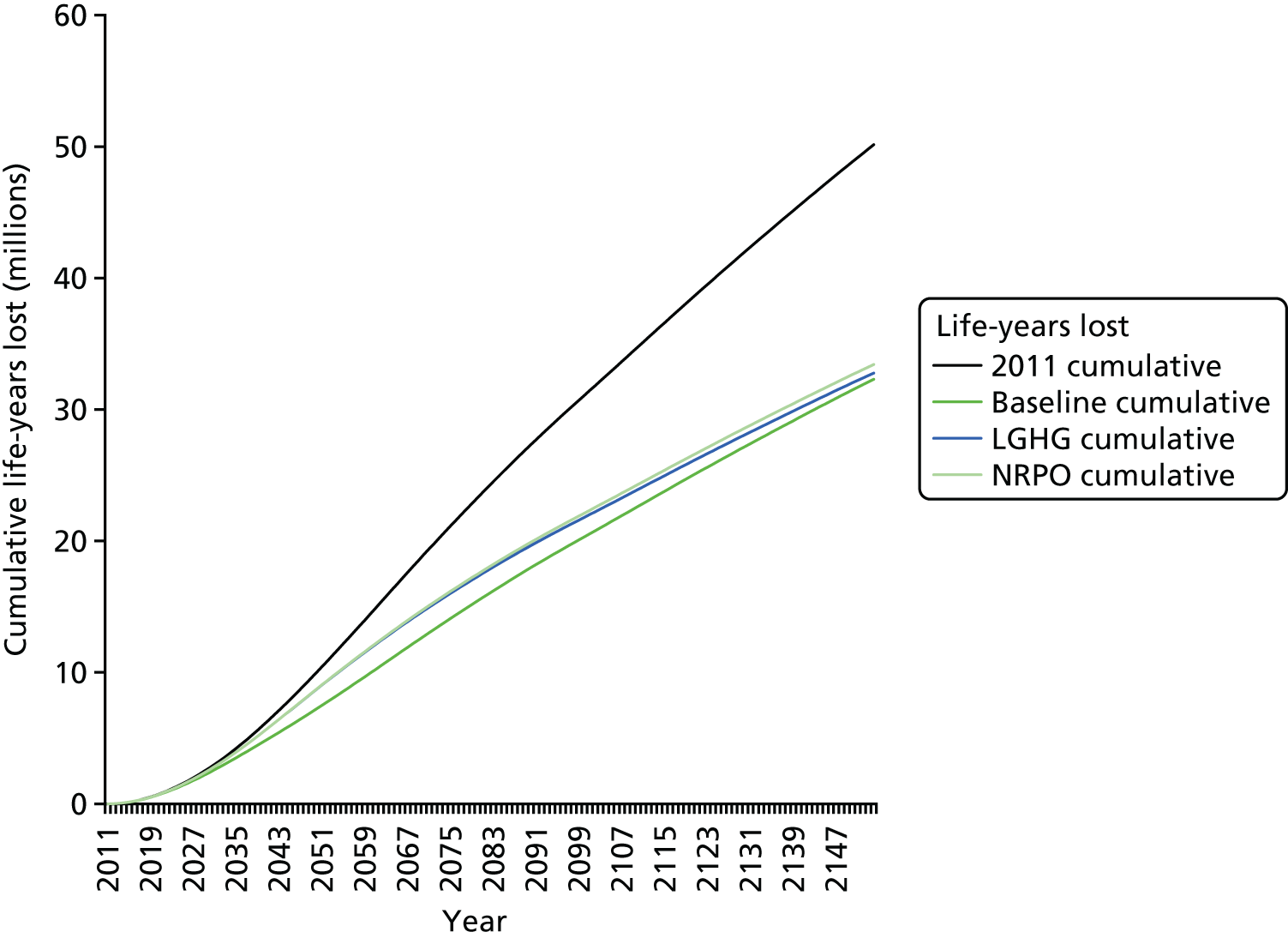
FIGURE 37.
Life-years saved across the GB population (no migration), with projected new births, 2011–2154, for anthropogenic PM2.5 in three greenhouse gas reduction scenarios, compared with 2011 anthropogenic PM2.5 concentrations remaining unchanged, RR 1.06 per 10 µg/m3, US EPA lag.
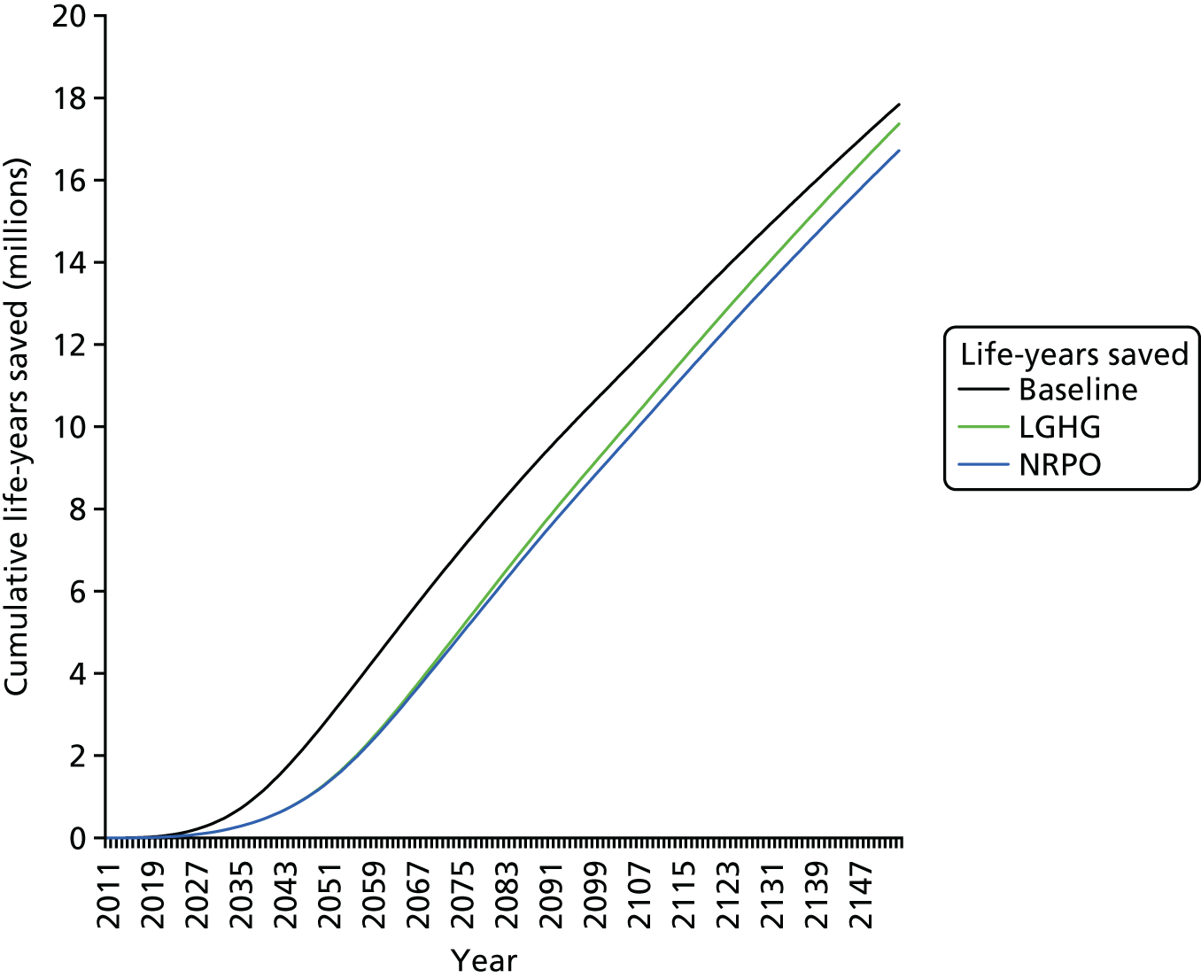
Although the life-years gained are broadly similar, it can be seen that it is actually the baseline (current policies) scenario that gains the most life-years (17.8 million). Although PM2.5 concentrations are lower for the NRPO and LGHG scenarios than the base case in 2050, the concentrations do not actually reduce as much in these scenarios in 2035 compared with the baseline scenario. This is because of the increase in biomass emissions discussed above.
Having illustrated that life-years are gained for the base case, Table 15 shows the comparison of the NRPO and LGHG scenarios more clearly. Figure 37 also shows the development of the gains/losses over time.
| Scenario | Year | Change in GB population-weighted mean concentrations compared with 2011 (µg/m3) | Total life-years saved compared with the baseline (current policies) scenario whole population with new births, 2011–2154 | ||
|---|---|---|---|---|---|
| Male | Female | Total | |||
| NRPO | 2011 | 0 | –579,199 | –543,006 | –1,122,206 |
| 2035 | 2.72 | ||||
| 2050 | –0.41 | ||||
| LGHG | 2011 | 0 | –231,715 | –240,086 | –471,802 |
| 2035 | 2.72 | ||||
| 2050 | –0.57 | ||||
Table 15 shows that both scenarios are actually worse than the baseline case, with current policies showing 1.1 million and 470,000 life-years lost (negative life-years gained) for NRPO and LGHG, respectively, compared with the base case. Figure 36 shows that the cumulative life-years lost in the base case (current policies) accumulate more slowly than either the constant 2011 concentration results or in the NRPO and LGHG scenarios, although the last two get closer to each other for the later years. Figure 37 also shows this. It is worth remembering that there is a delay before the full benefits of concentration reductions are achieved. This is not just attributable to a lag between exposure and effect, but also because the greatest gains occur when mortality rates are highest (i.e. in the elderly). Thus, although by 2050 the concentration reduction is a little bit greater for the NRPO and LGHG scenarios and this difference in concentration is maintained unchanged after 2050, it is another 30–40 years before the cumulative life-years gained start to ‘catch up’ with the base-case scenario. Similarly, when comparing the NRPO and LGHG scenarios with each other, their concentrations start to diverge in 2035, but it is not until 2070 or so before the slopes start to diverge noticeably from each other. When the concentration differences first occur, the effect will be strongly apparent only in the elderly portion of the population but, over time, more and more of the original population become elderly and thus affected by the maintained change. This is why long time periods are needed for the analysis. These effects can be more clearly illustrated by plotting the life-years lost per year during the period of analysis relative to the baseline scenario. This quantity is shown in Figure 38 and shows the effect of the increase in biomass use in the NRPO and LGHG scenarios compared with the baseline scenario. The large increase in life-years lost per year peaks in the 2040s before becoming ‘life-years gained’ well into the period beyond the CCA target on this analysis, around 2070.
FIGURE 38.
Life-years lost per year from long-term exposure to anthropogenic PM2.5 relative to the baseline scenario.
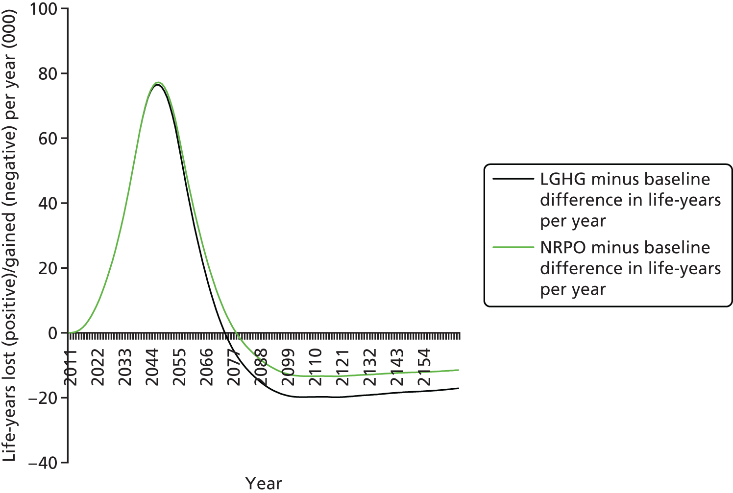
Total life-years across the population is the most appropriate metric for cost–benefit analysis of policies, as it captures effects in the entire population. However, it is a difficult type of metric to communicate as it is difficult to judge what is a ‘small’ answer or a ‘large’ answer. Life expectancy from birth is a more familiar concept for the general public, although it captures effects only on those born on a particular date. Results for life expectancy from birth are shown in Table 16.
| Scenario | Year | GB population-weighted mean concentrations (µg/m3) | Loss of life expectancy from birth compared with baseline mortality rates, 2011 birth cohort followed for 105 years (weeks) | |
|---|---|---|---|---|
| Male | Female | |||
| Concentration does not reduce from 2011 levels | 2011 | 9.31 | 29.5 | 25.8 |
| 2035 | 9.31 | |||
| 2050 | 9.31 | |||
| Base case (current policies) | 2011 | 9.31 | 18.5 | 16.2 |
| 2035 | 4.74 | |||
| 2050 | 5.77 | |||
| NRPO | 2011 | 9.31 | 17.6 | 15.3 |
| 2035 | 7.46 | |||
| 2050 | 5.36 | |||
| LGHG | 2011 | 9.31 | 17.1 | 14.9 |
| 2035 | 7.46 | |||
| 2050 | 5.20 | |||
This shows that loss of life expectancy from birth would be about 26–30 weeks (6–7 months) if 2011 PM2.5 concentrations were unchanged, but improves by about 9–11 weeks for the base case and by 10–12 weeks for the NRPO and LGHG scenarios. This is only a small improvement over the base case. Considering the confidence intervals in the CRFs, the results varied from one-sixth to almost twice these values when using the plausibility interval from a hazard ratio of 1.01 to one of 1.12.
Modelling scale can affect modelled concentrations and, hence, health impact. However, as PM2.5 is fairly spatially homogeneous as a result of regional contributions of PM2.5, changes in modelling scale had only a small effect when tested on the NRPO scenario. GB population-weighted mean concentrations in 2035 were 7.33 µg/m3 for 10-km grid-modelled concentrations in both rural and urban areas and 7.44 µg/m3 for 10-km rural/20-m urban modelling, compared with 7.46 µg/m3 for the 10-km grid rural/2-km grid urban modelling used for all the scenarios. The equivalent figures for 2050 were 5.26, 5.36 and 5.36 µg/m3. Unsurprisingly, these differences reduced the answers in terms of life-years lost by only 3% for the 10-km rural and 10-km urban modelling and by 0.1% for the 10-km rural/20-m urban modelling. This was based on concentrations averaged up to ward level, which will average out some of the exposure contrasts, perhaps explaining the relatively small impact of finer-scale, 20-m, modelling (see Table 10).
Although the results discussed in this section refer to PM2.5, and it is likely that PM2.5 itself is a significant contributor to the effects, it is possible that the effects of other traffic pollutants are being reflected to some extent.
Impact of nitrogen dioxide (and possibly other traffic or combustion pollutants)
The results for NO2 are given in Table 17. The exact pollutants responsible for the associations in reality are unclear, although it is thought likely that NO2 itself makes some contribution. 100 References to effects of changes in NO2 concentrations in the following text should be read with this in mind. The results are given as a range from using a cut-off (counterfactual) point of 5 µg/m3, to assuming effects can be extrapolated down to zero.
| Scenario | Year | NO2 GB population-weighted mean concentrations (µg/m3) | Total life-years lost compared with baseline mortality rates, whole population with new births, 2011–2154 | ||
|---|---|---|---|---|---|
| Male | Female | Total | |||
| Concentration does not reduce from 2011 levels | 2011 | 9.53–14.4 | 9,439,172 to 13,322,689 | 8,243,553 to 11,689,378 | 17,682,726 to 25,012,067 |
| 2035 | 9.53–14.4 | ||||
| 2050 | 9.53–14.4 | ||||
| Base case (current policies) | 2011 | 9.53–14.4 | 6,015,864 to 9,856,596 | 5,260,688 to 8,667,812 | 11,276,553 to 18,524,408 |
| 2035 | 2.44–6.98 | ||||
| 2050 | 6.43–11.25 | ||||
| NRPO | 2011 | 9.53–14.4 | 3,408,301 to 7,145,468 | 2,976,271 to 6,291,577 | 6,384,572 to 13,437,045 |
| 2035 | 2.82–7.37 | ||||
| 2050 | 2.55–7.08 | ||||
| LGHG | 2011 | 9.53–14.4 | 2,370,507 to 6,019,928 | 2,088,795 to 5,326,466 | 4,459,303 to 11,346,394 |
| 2035 | 2.82–7.37 | ||||
| 2050 | 1.33–5.65 | ||||
The calculations use a RR (hazard ratio) of 1.017 per µg/m3 of NO2, with a confidence interval of 1.007 to 1.027 (i.e. from roughly 40% to 1.5 times the numbers given). The effects are unlikely to represent effects of NO2 alone, as this pollutant is closely correlated with other traffic/combustion pollutants.
As expected, the results assuming no effect < 5 µg/m3 are smaller. In addition, the lower the population-weighted mean concentration gets, the more proportional difference the cut-off point makes to the results. This is because a greater number of areas are < 5 µg/m3 and set to zero in the calculations. The ‘minus 5’ population-weighted mean varies from 66% (for 2011) to 24% (LGHG, 2050) of the zero cut-off point result. The life-years lost results range from 71% (2011 constant) to 39% (LGHG) of the zero cut-off point result. (The rank order for the life-year results follows that of the population-weighted mean concentrations, but the proportions do not match exactly.) There are probably a variety of reasons for this: the population-weighted means vary over time; the relationship between change in population-weighted mean and change in hazard rate is not linear; and the life table calculations take account of some wards within a local authority, but not others, falling < 5 µg/m3 over time, including the intervening years between 2011, 2035 and 2050.
In contrast to the results using the PM2.5 coefficient, there is more difference between the scenarios ranging from 4.5 million life-years lost (LGHG, 5 µg/m3 cut-off point) to 25 million life-years lost (2011 constant, no cut-off point), or within the same cut-off point assumption (11–25 million life-years lost). Overall, life-years lost are lower than for PM2.5, the smaller size of the coefficient compensating for the slightly larger NO2 concentration in 2011.
Compared with no change in 2011 concentrations (Table 18), the reduction in population-weighted mean concentrations is now much closer between the zero and 5 µg/m3 cut-off points, although as the reductions get larger (and more areas fall < 5 µg/m3), there is more of a difference (the extent of the reduction is ‘blunted’ by the cut-off point at 5 µg/m3).
| Scenario | Year | Difference in NO2 GB population-weighted mean concentrations (µg/m3) | Total life-years saved compared with 2011 concentrations maintained, whole population with new births, 2011–2154 | ||
|---|---|---|---|---|---|
| Male | Female | Total | |||
| Baseline (current policies) | 2011 | 0 | 3,423,308 to 3,466,093 | 2,982,865 to 3,021,566 | 6,406,173 to 6,487,659 |
| 2035 | –7.09 to –7.42 | ||||
| 2050 | –3.1 to –3.15 | ||||
| NRPO | 2011 | 0 | 6,030,871 to 6,177,221 | 5,267,282 to 5,397,801 | 11,298,154 to 11,575,022 |
| 2035 | –6.71 to –7.03 | ||||
| 2050 | –6.98 to –7.32 | ||||
| LGHG | 2011 | 0 | 7,068,665 to 7,302,761 | 6,154,758 to 6,362,912 | 13,223,423 to 13,665,673 |
| 2035 | –6.71 to –7.03 | ||||
| 2050 | –8.2 to –8.75 | ||||
The life-years gained vary by a factor of 2, with the LGHG scenario giving considerably more benefits (13.2–13.6 million life-years saved) than the base case (6.4–6.5 million life-years saved). The gains are smaller than for PM2.5, despite the larger concentration changes, as a result of the smaller coefficient.
Comparing the NRPO and LGHG scenarios with the base case in Table 19, the population-weighted mean concentrations are actually very slightly higher for the NRPO and LGHG scenarios than in the base case in 2035, but by 2050 these two scenarios lead to substantially lower concentrations. Compared with PM2.5, concentrations of which are a large amount higher in 2035 and a small amount lower in 2050, the net result for NO2 is for gains in life-years. The gains for the LGHG scenario are greater, at 6.8–7.2 million life-years, than for the NRPO scenario (4.9–5.1 million life-years).
| Scenario | Year | Difference in NO2 GB population-weighted mean concentrations (µg/m3) | Total life-years saved compared with the base case, whole population with new births, 2011–2154 | ||
|---|---|---|---|---|---|
| Male | Female | Total | |||
| NRPO | 2011 | 0 | 2,607,563 to 2,711,128 | 2,284,417 to 2,376,235 | 4,891,981 to 5,087,363 |
| 2035 | 0.38 to 0.39 | ||||
| 2050 | –3.88 to –4.17 | ||||
| LGHG | 2011 | 0 | 3,645,357 to 3,836,668 | 3,171,893 to 3,341,346 | 6,817,250 to 7,178,014 |
| 2035 | 0.38 to 0.39 | ||||
| 2050 | –5.1 to –5.6 | ||||
Figure 39 shows that, with the sharper concentration changes from 2035 to 2050, the impact of the scenarios diverge more obviously than for PM2.5 from about 2050. The pattern is similar for the 5 µg/m3 cut-off point, at a smaller level of life-years lost (Figure 40). Figure 41 shows the comparison with 2011 concentrations remaining unchanged from 2011 and Figure 42 plots the cumulative life-years lost compared with baseline mortality rates with and without a cut-off point on the same graph.
FIGURE 39.
Cumulative life-years lost for four NO2 scenarios across the GB population (no migration), with projected new births, compared with life-years lived with baseline mortality rates (incorporating mortality improvements over time) 2011–2154. RR 1.017 per 10 µµg/m3, US EPA lag, no cut-off point.
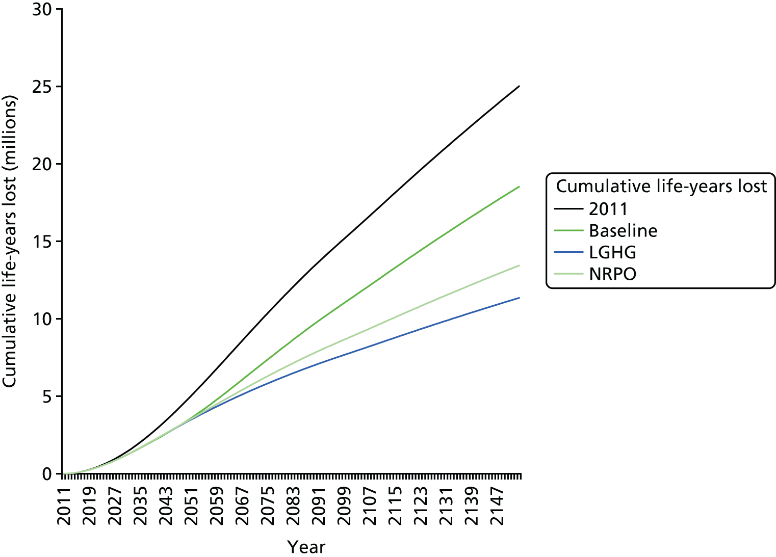
FIGURE 40.
Cumulative life-years lost for four NO2 scenarios across the GB population (no migration), with projected new births, compared with life-years lived with baseline mortality rates (incorporating mortality improvements over time) 2011–2154. RR 1.017 per 10 µg/m3, US EPA lag, 5 µg/m3 cut-off point.
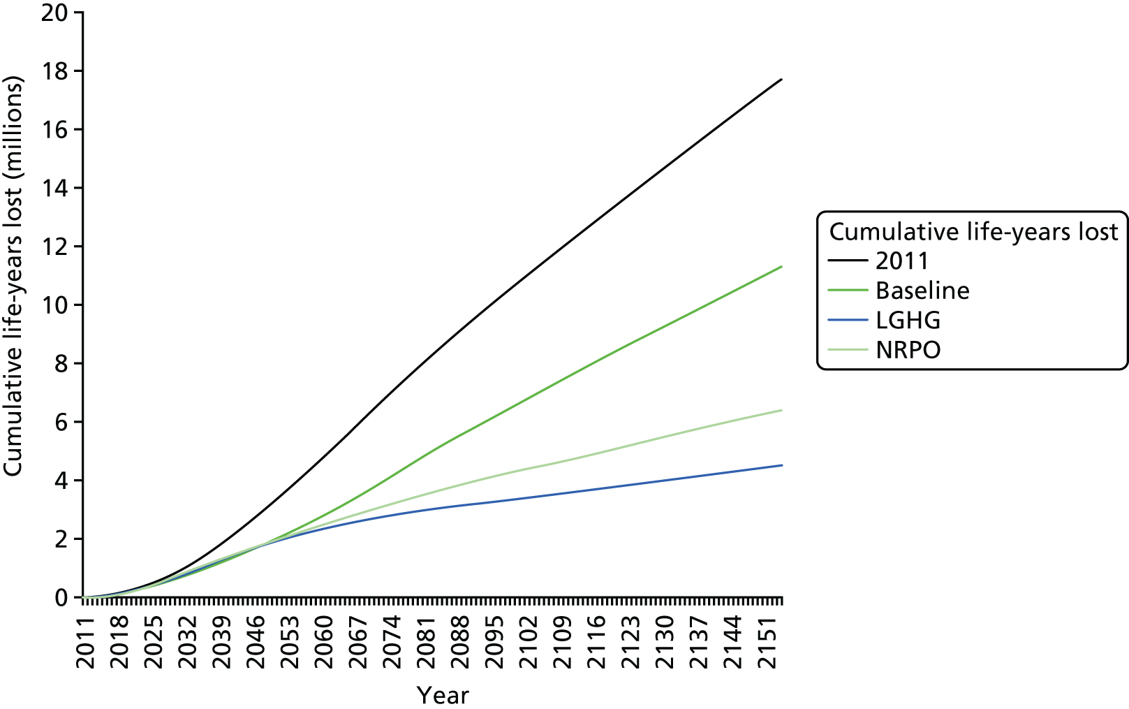
FIGURE 41.
Life-years saved across the GB population (no migration), with projected new births, 2011–2154, for NO2 in three greenhouse gas reduction scenarios, compared with 2011 NO2 concentrations remaining unchanged, RR 1.017 per 10 µg/m3, US EPA lag, no cut-off point.
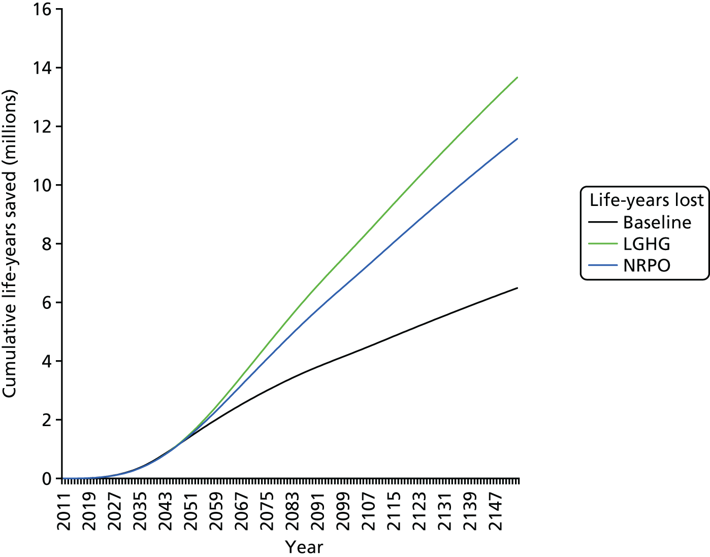
FIGURE 42.
Cumulative life-years lost across the GB population (no migration), with projected new births, 2011–2154, for NO2 in an example greenhouse gas reduction scenario (LGHG), compared with life-years lived with baseline mortality rates (incorporating mortality improvements over time), RR 1.017 per 10 µg/m3, US EPA lag, with and without cut-off point of 5 µg/m3.
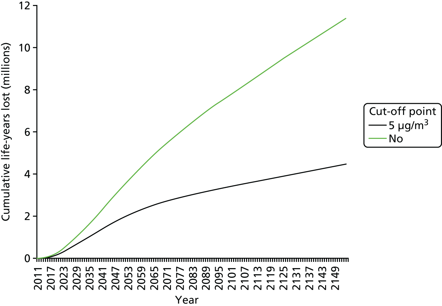
Loss of life expectancy from birth is shown in Table 20.
| Scenario | Year | NO2 GB population-weighted mean concentrations (µg/m3) | Loss of life expectancy from birth compared with baseline mortality rates, 2011 birth cohort followed for 105 years (weeks) | |
|---|---|---|---|---|
| Male | Female | |||
| Concentration does not reduce from 2011 levels | 2011 | 9.53–14.4 | 10.7 to 15 | 9.3 to 13.1 |
| 2035 | 9.53–14.4 | |||
| 2050 | 9.53–14.4 | |||
| Base case (current policies) | 2011 | 9.53–14.4 | 7.1 to 11.3 | 6.2 to 9.9 |
| 2035 | 2.44–6.98 | |||
| 2050 | 6.43–11.25 | |||
| NRPO | 2011 | 9.53–14.4 | 3.2 to 7.3 | 2.8 to 6.4 |
| 2035 | 2.82–7.37 | |||
| 2050 | 2.55–7.08 | |||
| LGHG | 2011 | 9.53–14.4 | 1.7 to 5.7 | 1.4 to 4.9 |
| 2035 | 2.82–7.37 | |||
| 2050 | 1.33–5.65 | |||
This shows that loss of life expectancy from birth would be about 9–15 weeks (2–3.5 months) if 2011 NO2 concentrations were unchanged, but improves by about 3–4 weeks for the base case, by 7–8 weeks for the NRPO scenario and by 8–9 weeks for the LGHG scenario. The loss of life expectancy from birth would be very small with respect to NO2 (and/or pollutants with which it is closely correlated) after implementation of the NRPO or LGHG scenarios compared with the base case. Results varied from 41% of the central estimate to 1.6 times the relevant values with or without a cut-off point when using the confidence interval from a hazard ratio of 1.007 to one of 1.027.
The plot of life-years lost per year is shown in Figure 43 and the difference between this plot and that for PM2.5 is very clear. Apart from a very small loss in life-years at the beginning of the period, before the larger emission reduction measures take effect, life-years are saved in both scenarios compared with the baseline, with a relatively small difference with and without a cut-off point.
FIGURE 43.
Life-years lost per year for NO2, relative to the baseline scenario.
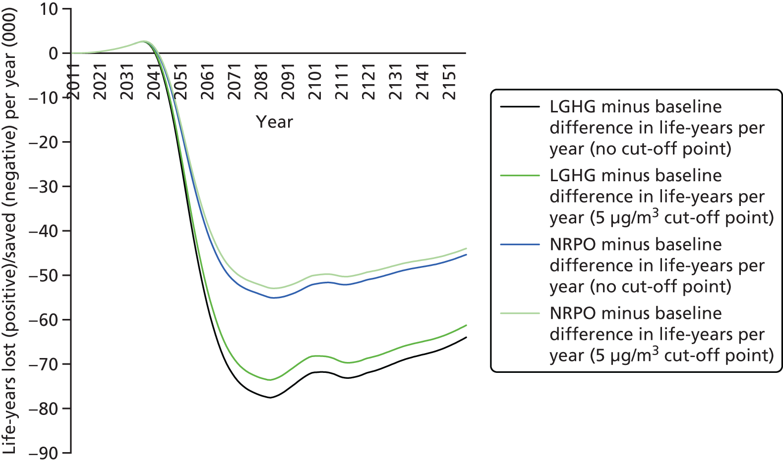
The sensitivity on modelling scale for the NRPO scenario showed GB population-weighted mean concentrations of NO2 (no cut-off point) in 2035 were 6.93 µg/m3 for 10-km grid modelled concentrations in both rural and urban areas and 7.37 µg/m3 for 10-km rural/20-m urban modelling, compared with 7.37 µg/m3 for the 10-km rural/20-km urban modelling used for all the scenarios. The equivalent figures for 2050 were 6.72, 7.07 and 7.08 µg/m3. The differences are slightly greater than for PM2.5, as would be expected for a more spatially homogeneous pollutant. These differences reduced the life-years lost by 8% for the 10-km rural and 10-km urban modelling and increased the life-years lost by 0.3% for the 10-km rural/20-m urban modelling. For NO2, omitting more detailed 2-km modelling of urban areas underestimates the impact, but moving up to 20-m modelling from 2 km makes less of a difference. Again, averaging up to ward level probably averages out some exposure contrasts from the 20-m modelling (see Table 10). The life-years lost results for NO2 with a cut-off point (2011 baseline) were 12% lower for the 10 km/10 km modelling and 3% higher for the 10 km/20 m modelling. The respective values for the NRPO scenario were 17% lower and 1% higher. As expected, these are larger differences than for NO2 without a cut-off point, as areas close to 5 µg/m3 may be above or below this cut-off point according to modelling scale.
Impact of ozone
In considering the long-term impact of O3, we need to be aware of the uncertainties surrounding the epidemiological evidence. The WHO’s HRAPIE study95 recommended a CRF as set out in Table 11, but it was graded as B (a measure of confidence), compared with, for example, the CRF for PM2.5 which was graded A*. We therefore consider this quantification as a sensitivity calculation and will discuss the results in less detail than for PM2.5 and NO2.
The results are shown in Table 21.
| Scenario | O3 GB population-weighted mean concentrations (µg/m3) | Total life-years lost compared with baseline mortality rates, whole population with new births, 2011–2154 | ||
|---|---|---|---|---|
| Male | Female | Total | ||
| Concentration does not reduce from 2011 levels | 34.7 | 3,146,765 | 2,692,044 | 5,838,808 |
| Baseline (current policies) | 27.7 | 2,536,606 | 2,176,301 | 4,712,907 |
| NRPO | 28.7 | 2,655,877 | 2,273,953 | 4,929,830 |
| LGHG | 28.7 | 2,669,961 | 2,284,088 | 4,954,049 |
The same results are shown graphically in Figure 44.
FIGURE 44.
Cumulative life-years lost associated with long-term O3 exposure compared with baseline mortality rates.
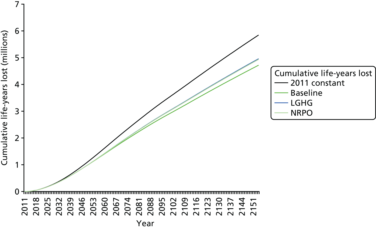
The overall impact is of a similar order to that estimated for NO2 with a cut-off point of 5 µg/m3 and the baseline (no further measures) scenario shows fewer life-years lost than the two CCA-compliant scenarios. The reason for this is probably because of the lower NOx emissions in the two CCA-compliant scenarios, LGHG and NRPO, in which the effect of removing the ‘titration’ effect of NO and O3 is having an effect on the higher O3 concentrations.
The loss of life expectancy from birth in 2011 if O3 concentrations remain unchanged was estimated at around 3 weeks, with a very slight improvement for the scenarios to 2–3 weeks. This is an average across all those born in 2011, and, particularly as the O3 coefficient only relates to respiratory mortality, it is more likely that there is a greater loss of life expectancy for some, while others are unaffected.
The impact on health of long-term O3 exposure, albeit uncertain, in all three future scenarios is significantly smaller than that of PM2.5, and that of NO2 with no cut-off point, by factors of around 6 and around 3–4, respectively.
The question of the existence of a threshold for O3 effects is extremely important. In considering the impact of short-term exposures to O3, COMEAP96 did not recommend qualifying the effects of long-term exposures, but recommended a short-term CRF for all-cause mortality and recommended using no threshold (the COMEAP approach was to meta-analyse studies of all-cause mortality, whereas WHO HRAPIE95 work selected a particular study that showed effects on respiratory mortality). This is a significant statement as noted by Heal et al. ,130 as an approximate calculation shows. Taking the COMEAP CRF of 0.34% increase in mortality per 10 µg/m3 increase in the daily maximum 8-hour mean concentration and assuming linearity, the mortality outcome is determined by the annual mean concentration, which is of the order of 100 µg/m3 (see Table 10). Assuming a UK population of 65 million and an annual mortality base rate of 1%, one estimates the number of premature deaths from short-term exposure to O3 as ≈22,000, a figure broadly comparable to the figure of ≈29,000 premature deaths estimated from long-term exposure to PM2.5. 59 Heal et al. ,130 in a study of 2003 O3 concentrations, derived a figure of ≈11,500 DBF using an earlier CRF recommended by WHO. We intend to do more investigation of the effects of changes in short-term exposure to pollutants as a result of climate change policies in further development of this work.
Overall impact of long-term exposure to air pollution
Calculations were done for each pollutant separately so that results could be recombined in various ways subsequently. The overlap between pollutants is a particular uncertainty because of close correlations between pollutants and difficulties in interpreting multipollutant models in the presence of differing levels of measurement error between pollutants. In addition, if changes in risks from one pollutant change the mortality rates, population size and age distribution, this would in turn affect the impact of a different pollutant. We intend to investigate this in further work.
Effects of long-term exposure to PM2.5 are well established. Recent epidemiological studies showing associations with NO2 suggest the possibility that there may be a small additional effect on mortality better reflected by NO2 than by PM2.5. This does not mean that this possible additional effect is as a result of NO2 alone: intraurban NO2 exposure contrasts probably act as a better marker for traffic pollutants (including NO2 itself, primary PM, ultrafine particles, PAHs, VOCs, carbon monoxide, etc.) than PM2.5 (which includes both regional and local sources). Separation of correlated pollutants in epidemiological studies is very challenging, so the results for the different pollutants need to be seen as estimating health impact from different angles rather than strictly exact effects from particular pollutants.
The issue of adding results for NO2 to PM2.5, or not, is particularly pertinent in this case as the benefits from NO2 concentration reductions would outweigh the adverse health impact from PM2.5, giving net life-years saved of 3.8–4 million for the NRPO scenario and 6.3–6.7 million for the LGHG scenario. But could the uncertainty in the NO2 concentration–response function mean that these benefits would not outweigh the PM2.5 adverse impacts? What if the effects represented by PM2.5 actually overlapped considerably with the effects best represented by NO2 such that the benefits linked with NO2 were reduced? This overlap would need to be as high as 77% for the NRPO scenario and 93% for the LGHG scenario before the benefits linked with NO2 would not outweigh the adverse PM2.5 impacts. The outweighing of the adverse health impact does not need to be on the basis of assuming an effect of NO2 alone as some other traffic pollutants are also likely to be reduced by policies, such as a shift to electric vehicles. However, in some senses, these discussions of overlap are beside the point. The increase in biomass element of the policies is delivering adverse impacts from PM2.5, for which the health evidence is strongest, and it would be possible to design policies to avoid this.
Jerrett et al. 126 found that the association of O3 with respiratory mortality was independent of that from PM2.5, with PM2.5 showing no effect on respiratory mortality after control for O3. NO2 was not examined in this study, but in other studies,127,131 using three pollutant models, O3 associations are robust to control for NO2. These types of combined pollutant risk models may be important approaches for future impact analysis. The overall evidence on long-term exposure to O3 and mortality is somewhat contradictory,96 so this is a sensitivity analysis, but in that context it seems reasonable to add the results to those for PM2.5. However, the impact of O3 was small so this probably would not affect the conclusions. (Short-term exposure impact of O3 needs to be added and these could be important.) Table 22 provides some commentary on ways that results could be combined, but important caveats have to be noted. Overall, we recommend that health impact is described separately for the different pollutants before discussing the balance between them. An overall total, without comment, would omit the fact that quantification of effects of long-term exposure to PM2.5 is more robust, whereas quantification of effects of long-term exposure to O3 and NO2 is more uncertain; furthermore, the latter is probably overestimated.
| Analyses | Pollutant | Comment | ||
|---|---|---|---|---|
| PM2.5 | NO2 | O3 | ||
| Core | ✓ | – | – | May be a small underestimate but well-established pollutant–outcome pair. Include effects of short-term exposure to NO2 and O3 on mortality when long-term exposure is not included |
| Sensitivity 1 | ✓ | ✓ | – | It is likely that there is substantial overlap between the effects of PM2.5 and NO2. Although the NO2 coefficient is adjusted for PM2.5, it is not adjusted for effects of other traffic pollutants. In addition, the PM2.5 coefficient is not adjusted for NO2. Thus, the combined result is likely to be an overestimate |
| Sensitivity 2 | ✓ | – | ✓ | As with the coefficient for PM2.5, the O3 coefficient is also from a single pollutant model. Association seemed to be independent of PM2.5 with little apparent overlap126 |
Chapter 8 Impact of air pollution scenarios on inequalities
Background
Environmental inequality, the concept that more vulnerable individuals, communities and subpopulations are more likely to be exposed to higher levels of environmental pollution, is well documented, particularly in relation to air pollution. 132,133 Environmental inequality implies disadvantages in subpopulations and certain communities because increased levels of both pollution exposure and socioeconomic deprivation may lead to impaired health. 134 Social gradients in health are well established in England, and it has been estimated that between 1.3 and 2.5 million years of life are lost because of health inequalities. 135 Socially and economically disadvantaged people may experience increased susceptibility to the negative air pollution-related health effects, ranging from conditions such as respiratory irritation and cardiovascular disease to premature death, as a result of higher underlying baseline disease rates in deprived communities. 136 Some studies have shown this effect modification on morbidity and mortality risks, in particular for urban areas, where individuals of high social class are not as affected by the negative health effects of air pollution as are individuals of lower social classes. 137 The relationships between the geographical distribution of vulnerable communities and air pollution are, however, more complex than often implied. 138 They vary considerably by geographical area,139 by environmental pollutant140–142 and over time. 143
Understanding how air pollution exposure differs between subpopulations is important for environmental policy and public health, not only to reduce the average risk across the population but, also, to safeguard that no population subgroup such as deprived or ethnic minorities is more burdened than others. 144
Here, we aim to investigate small area associations of air pollution exposures with socioeconomic deprivation and ethnicity and explore the underlying geographical relationships in environmental inequality. We analyse variations in exposure to air pollution by subpopulation across GB and explore if differences in observed national patterns vary by country and government region. This allows us to identify areas at highest risk of environmental inequality for each of the air pollution scenarios.
Data and methods
Study area
The small area unit for this study is the ward 2011 level. Wards are one of the dissemination units for which output statistics from the 2011 census are reported for England and Wales by the ONS and for Scotland by the National Records of Scotland. There are 8941 wards in GB, with an average population of ≈3500. To analyse geographical differences across GB we stratified our analysis by country and, within England, by region, using the 2011 ONS region boundaries (Figure 45).
FIGURE 45.
Study area.
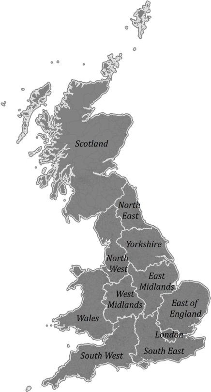
Air pollution exposure
We used air pollution maps at the 10-km/2-km resolution of annual mean concentrations for NO2, PM2.5, PM10 and daily maximum hourly (Dmax) NO2 as described in Chapter 5. For O3, we used both the long-term metric [i.e. the April–September average of the daily maximum 8-hour mean above 35 p.p.b. (equivalent to 70 µg/m3)] and the short-term metric (i.e. the annual average of the daily maximum 8-hour mean, with no threshold or cut-off point). We aggregated the modelled air pollution concentrations to ward 2011 level. The future scenarios have already been described above.
Population characteristics
We analysed routinely available population characteristics at the ward 2011 level focusing on socioeconomic status and ethnicity.
We used the Carstairs 2011 index as the area-level socioeconomic indicator. The Carstairs index is a composite measure of deprivation which is commonly used in epidemiological and health analysis. 145,146 The index consists of census variables which are available and consistent across the three countries of England, Scotland and Wales. The Carstairs index includes the following four variables:
-
unemployment – defined as unemployed males aged 16–74 years as a proportion of all economically active males aged 16–74 years
-
car ownership – defined as households which do not own a car as a proportion of all private households
-
overcrowding – defined as households with more than one person per room as a proportion of all households
-
low social class – defined as persons in households with household reference person aged 16–74 years in social class D or E as a proportion of all persons in households.
We calculated the Carstairs 2011 index following the methodology described by Carstairs and Morris147 using 2011 census data at the ward 2011 level. To compute the Carstairs deprivation score, the four input variables are combined by summing the standardised input variables. A higher Carstairs score thereby implies a greater degree of deprivation. To compare the difference in the relative ranking of all wards 2011 level, we categorised the Carstairs index into five equal groups (the Carstairs quintiles). Figure 46 shows the national distribution of Carstairs quintiles. We assume the same deprivation patterns observed in 2011 for the 2035 and 2050 scenarios, as relative deprivation patterns such as deprivation quintiles are fairly stable over time. 148
FIGURE 46.
Carstairs index using data from the 2011 census, standardised across all wards in GB (left) and ethnicity defined as % non-white based on 2011 census (right).
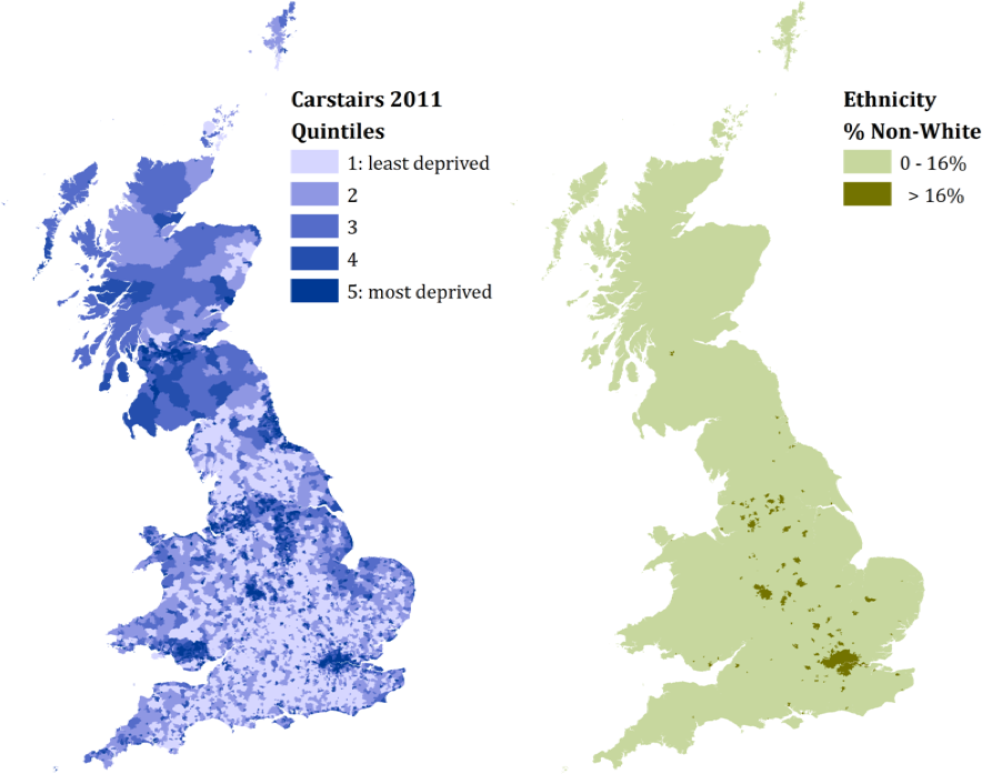
We categorised the wards (2011) according to their ethnic composition as white or non-white (see Figure 46). Using ethnicity information from the 2011 census, we defined white as white British, white Irish and white other. All other ethnic groups, including mixed ethnicity, were defined as non-white. We used a 16% cut-off point to differentiate between the two categories which reflects twice the national average of 8% non-white across all wards (2011) in GB. We analysed differences in air pollution levels by ethnicity for 2011 but not for the 2035 and 2050 scenarios, as ethnic composition of wards varies over time and no ethnicity projection information is available to conduct such analysis.
To analyse correlations of each air pollution variable with Carstairs index and ethnicity we used Pearson’s correlations, scatterplots and box-and-whisker plots. All statistical analyses were performed with open-source software R version 3.3.2 and R Studio (The R Foundation for Statistical Computing, Vienna, Austria).
Results
Descriptive statistics for annual mean NO2, Dmax NO2, O3, PM10 and PM2.5 concentrations at the ward 2011 level across GB are presented in Appendix 2. Concentrations were approximately normally distributed for all pollutants (histograms on request).
Associations of air pollution exposure and ethnicity
Table 23 shows the mean 2011 air pollution levels for white compared with non-white wards in 2011, for GB and the regions London, Wales and Scotland. We did not include results for England because patterns are very similar to those of GB overall. Similarly, we did not include explicitly here results for the regions, in order to minimise the amount of information in the report. These results are available on request from the authors. Both NO2 and PM2.5 concentrations are higher in non-white than in white wards in 2011. NO2 ratios between white and non-white wards are particularly high for GB (9.3 µg/m3 NO2 difference) and London (5.7 µg/m3 NO2 difference), whereas PM2.5 ratios are of a slightly lower magnitude and vary from 1.09 in London to 1.27 in GB. For O3, we observed slightly higher concentrations in white than in non-white wards (2011), but ratios between the wards (2011) categorised as white and non-white are generally low (ratio from 0.89 to 0.95).
| Region | Pollutant (µg/m3) | |||||||||||
|---|---|---|---|---|---|---|---|---|---|---|---|---|
| NO2 | PM2.5 | O3 long term | O3 short term | |||||||||
| White | Non-white | NO2 ratio | White | Non-white | PM2.5 ratio | White | Non-white | O3 ratio | White | Non-white | O3 ratio | |
| GBa | ||||||||||||
| 2011 | 11.2 | 20.5 | 1.83 | 9.0 | 11.4 | 1.27 | 35.8 | 32.2 | 0.90 | 97.1 | 91.0 | 0.94 |
| Londona | ||||||||||||
| 2011 | 20.3 | 26.0 | 1.83 | 11.6 | 12.7 | 1.09 | 34.3 | 30.9 | 0.90 | 92.3 | 88.1 | 0.95 |
| Walesa | ||||||||||||
| 2011 | 7.4 | 11.9 | 1.61 | 7.7 | 9.1 | 1.18 | 35.8 | 31.7 | 0.899 | 99.2 | 94.4 | 0.95 |
| Scotlanda | ||||||||||||
| 2011 | 5.5 | 9.2 | 1.67 | 4.6 | 5.6 | 1.22 | 34.6 | 30.7 | 0.89 | 99.8 | 94.0 | 0.94 |
Associations of air pollution exposure and deprivation
Figure 47 shows the relationship between selected air pollutants (NO2, PM2.5 and O3) and Carstairs deprivation scores, and the Pearson’s correlations between the variables for all wards (2011) in GB. Scatterplots for the other regions are available on request from the authors.
FIGURE 47.
Scatterplot showing relationship between Carstairs 2011 and pollutants (a–f) NO2; (g–l) PM2.5; (m–r) O3 (the long-term exposure metric); and (s–x) O3 no threshold (the short-term exposure metric), at ward 2011 and under different scenarios. Green indicates linear regression line and Pearson’s correlations are shown in blue.*Statistical significance p < 0.001.
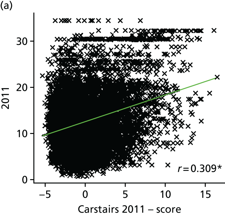
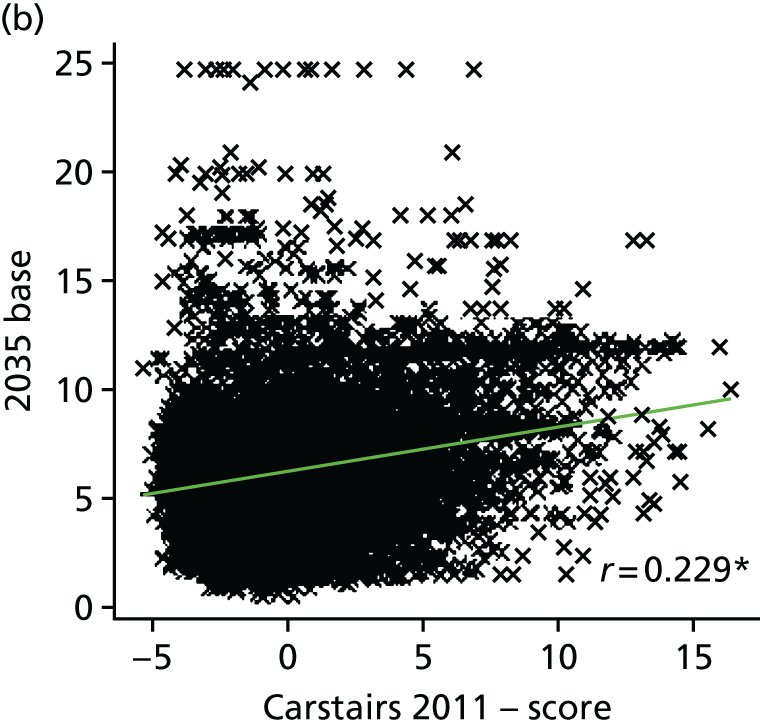

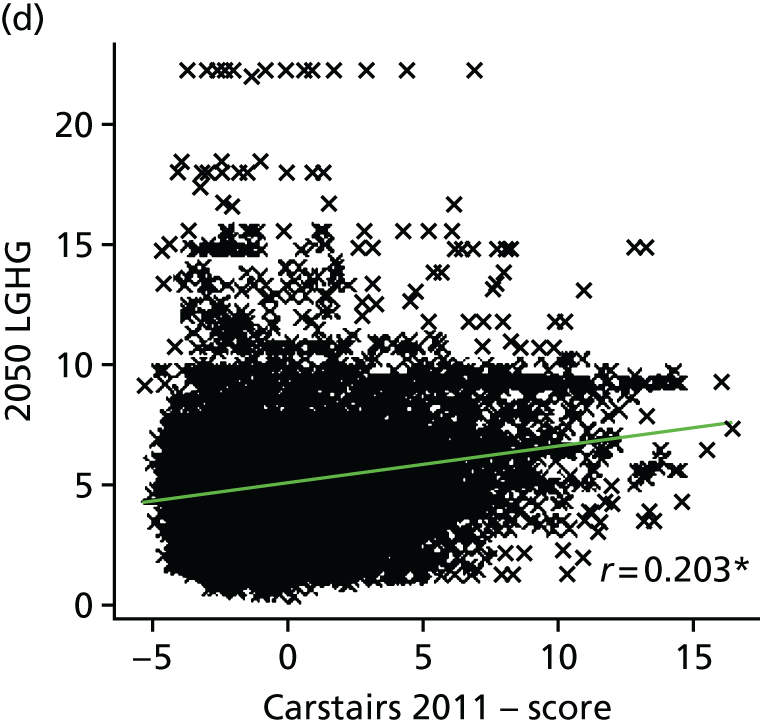
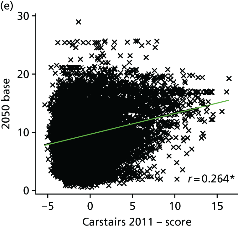
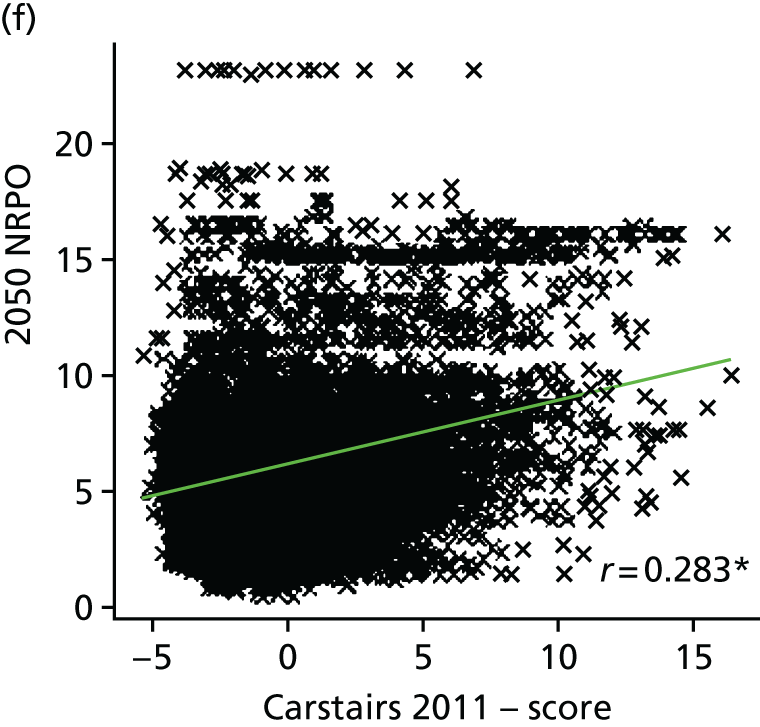
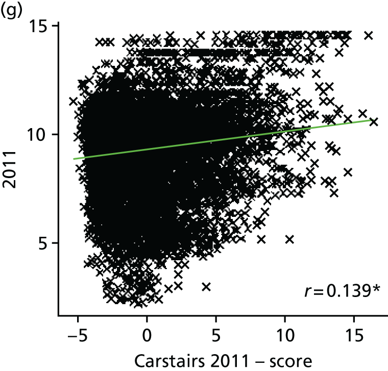

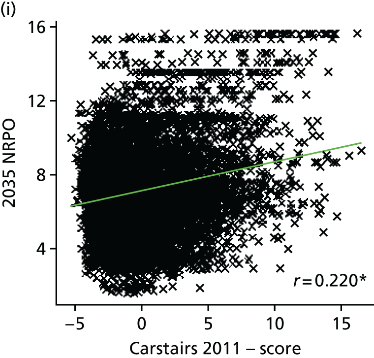
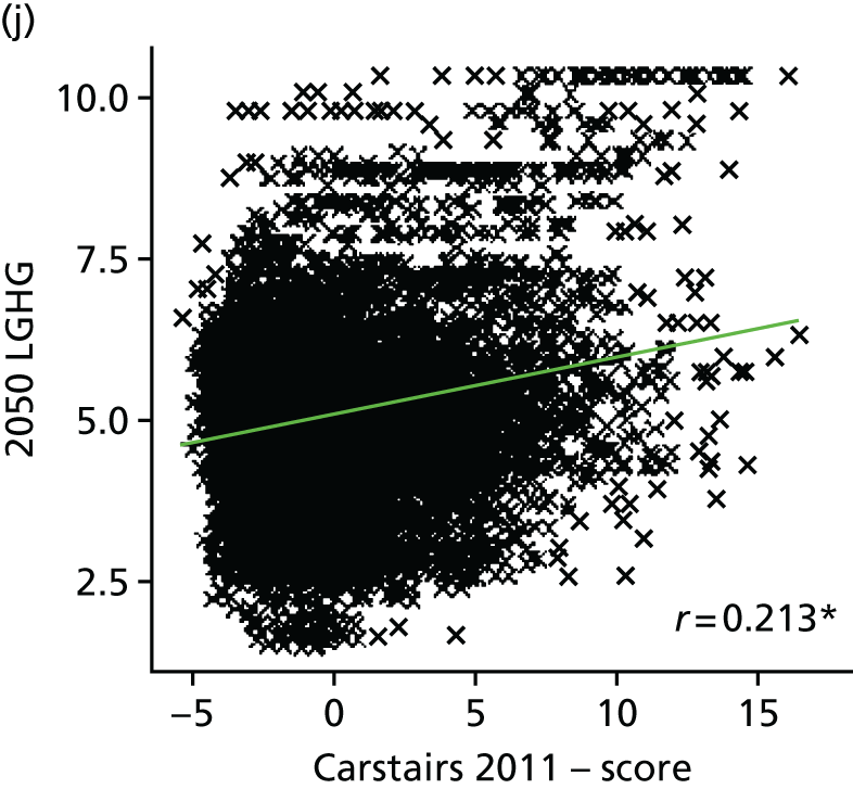

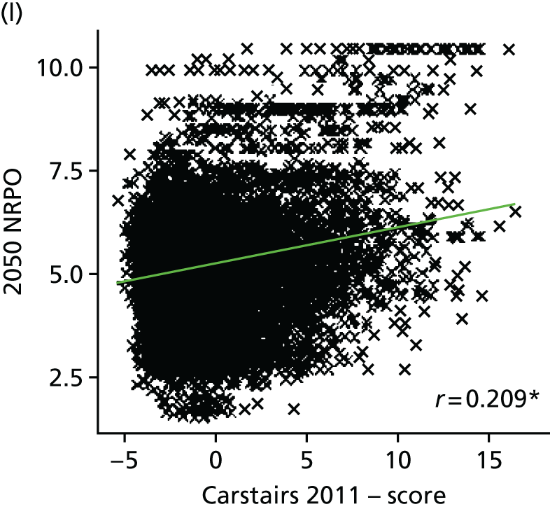
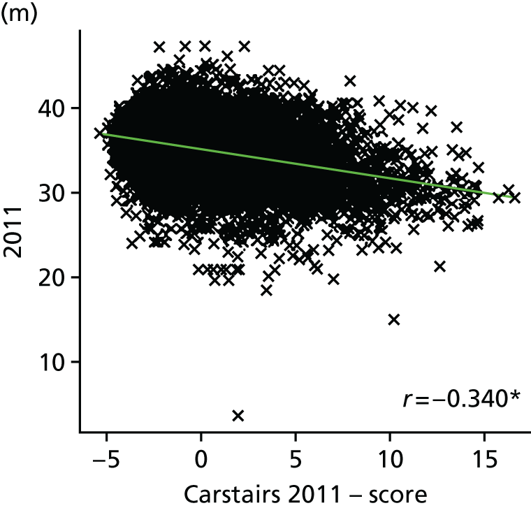

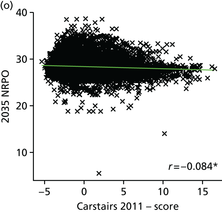
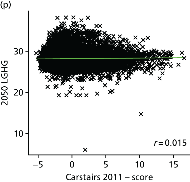
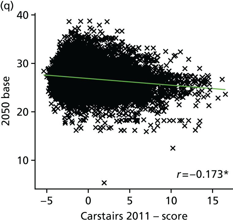


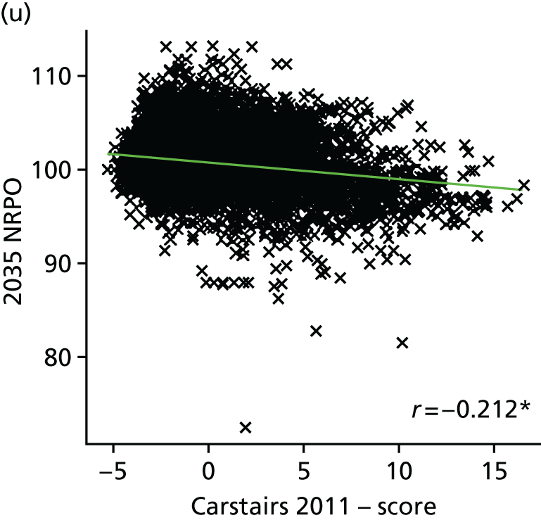
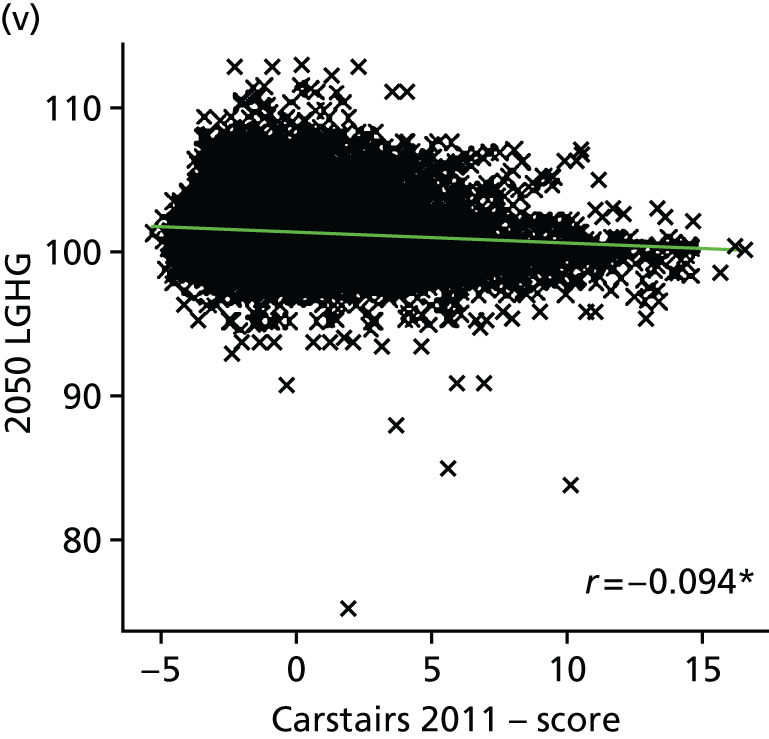
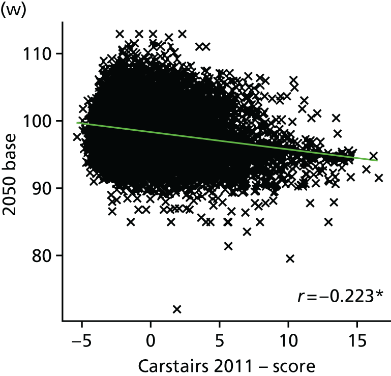
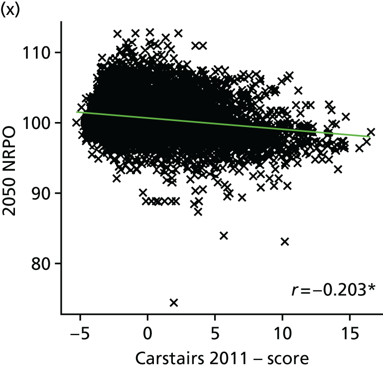
Nitrogen dioxide and PM2.5 concentrations are weakly correlated with the Carstairs score in 2011 (NO2, r = 0.309; PM2.5, r = 0.139), indicating that wards with a higher deprivation score have higher air pollution concentrations (although the spread across wards is very wide for both pollutants). For both pollutants, baseline scenarios have slightly weaker correlations than NRPO scenarios in 2035 and 2050. In contrast, in the LGHG scenario, the NO2 correlation with deprivation is the weakest of all the scenarios (r = 0.203) while for the PM2.5 correlation with deprivation is the highest of all 2050 scenarios (r = 0.213). All correlations for NO2 and PM2.5 are statistically significant with α = 0.001.
For O3, there is a weak negative correlation with Carstairs scores in 2011 using either O3 metric (with threshold, r = –0.340; without threshold, r = –0.303). For either of the scenarios, there were no, or very weak, correlations, which ranged from –0.173 to 0.015 for the O3 metric with threshold of 70 µg/m3 and from –0.223 to –0.094 for the O3 metric without a threshold.
Table 24 shows the mean air pollution levels for the highest compared with the lowest Carstairs quintile for GB and the regions London, Wales and Scotland (results for other regions are available on request from the authors). NO2 patterns by Carstairs quintile suggest that as air pollution levels decrease, so does the ratio of mean concentrations in the most deprived fifth of wards to those in the least deprived fifth of wards (2011) across GB. In London, this is true for the baseline and LGHG scenarios, whereas the ratio for the NRPO scenario increases. In Wales, however, the ratio of mean NO2 concentrations in the most deprived fifth of wards to those in the least deprived fifth of wards (2011) increases for all scenarios as NO2 levels decrease, and is highest for the LGHG scenario in 2050. PM2.5 patterns by Carstairs quintile show a similar trend for GB, Scotland, Wales and London. As PM2.5 levels drop, the ratio of the most deprived to the least deprived fifth of wards (2011) increases. This increase is particularly strong for the NRPO scenarios in all countries. In 2011, O3 levels in London were higher in the least deprived quintile than in the most deprived quintile. For all scenarios, this difference disappears and levels are almost the same in 2050. For other countries and GB, differences between the most and least deprived fifth of wards are minimal, with marginally higher exposure in the least deprived fifth of wards, except in Wales, where exposures are slightly higher in the most deprived fifth of wards.
| Region | Pollutant (µg/m3) | |||||||||||
|---|---|---|---|---|---|---|---|---|---|---|---|---|
| NO2 | PM2.5 | O3 with threshold | O3 without threshold | |||||||||
| Most deprived | Least deprived | NO2 ratio | Most deprived | Least deprived | PM2.5 ratio | Most deprived | Least deprived | O3 ratio | Most deprived | Least deprived | O3 ratio | |
| GB | ||||||||||||
| 2011 | 15.9 | 11.6 | 1.37 | 9.9 | 9.4 | 1.05 | 33.0 | 35.8 | 0.92 | 93.8 | 96.9 | 0.97 |
| 2035 baseline | 7.3 | 5.7 | 1.28 | 5.0 | 4.7 | 1.06 | 28.2 | 28.3 | 0.99 | 100.1 | 100.9 | 0.99 |
| 2035 NRPO | 7.9 | 5.8 | 1.36 | 8.1 | 7.0 | 1.16 | 27.9 | 28.2 | 0.99 | 99.6 | 100.8 | 0.99 |
| 2050 baseline | 11.8 | 9.0 | 1.31 | 6.6 | 6.1 | 1.08 | 25.9 | 27.0 | 0.96 | 96.8 | 98.7 | 0.98 |
| 2050 LGHG | 5.9 | 4.8 | 1.23 | 5.6 | 5.0 | 1.12 | 28.0 | 27.8 | 1.00 | 100.7 | 101.1 | 1.00 |
| 2050 NRPO | 7.7 | 5.6 | 1.38 | 5.8 | 5.2 | 1.12 | 27.7 | 27.9 | 0.99 | 99.6 | 100.7 | 0.99 |
| London | ||||||||||||
| 2011 | 26.8 | 19.5 | 1.37 | 12.9 | 11.5 | 1.12 | 30.3 | 35.6 | 0.85 | 87.4 | 93.8 | 0.93 |
| 2035 baseline | 11.0 | 8.8 | 1.25 | 6.9 | 5.9 | 1.17 | 28.9 | 30.1 | 0.96 | 98.7 | 100.9 | 0.98 |
| 2035 NRPO | 13.8 | 9.5 | 1.45 | 12.6 | 10.4 | 1.21 | 27.8 | 29.7 | 0.94 | 96.4 | 100.1 | 0.96 |
| 2050 baseline | 15.0 | 12.2 | 1.23 | 8.6 | 7.4 | 1.16 | 26.9 | 28.5 | 0.94 | 95.7 | 98.4 | 0.97 |
| 2050 LGHG | 8.9 | 7.2 | 1.24 | 8.3 | 6.9 | 1.20 | 29.0 | 29.8 | 0.97 | 99.9 | 101.5 | 0.98 |
| 2050 NRPO | 13.2 | 9.1 | 1.45 | 8.4 | 7.0 | 1.20 | 27.8 | 29.5 | 0.94 | 96.8 | 100.2 | 0.97 |
| Wales | ||||||||||||
| 2011 | 8.6 | 7.8 | 1.10 | 8.1 | 7.9 | 1.03 | 35.4 | 35.2 | 1.01 | 98.4 | 98.4 | 1.00 |
| 2035 baseline | 4.0 | 3.5 | 1.14 | 3.7 | 3.6 | 1.03 | 29.1 | 28.5 | 1.02 | 103.2 | 103.0 | 1.00 |
| 2035 NRPO | 4.0 | 3.4 | 1.18 | 6.2 | 5.5 | 1.13 | 29.1 | 28.5 | 1.02 | 103.2 | 102.9 | 1.00 |
| 2050 baseline | 6.1 | 5.4 | 1.13 | 4.9 | 4.8 | 1.02 | 27.7 | 27.4 | 1.01 | 101.6 | 101.6 | 1.00 |
| 2050 LGHG | 3.8 | 3.0 | 1.27 | 4.2 | 3.9 | 1.08 | 28.5 | 28.1 | 1.01 | 103.0 | 102.8 | 1.00 |
| 2050 NRPO | 4.3 | 3.5 | 1.23 | 4.3 | 4.0 | 1.08 | 28.6 | 28.2 | 1.01 | 102.8 | 102.7 | 1.00 |
| Scotland | ||||||||||||
| 2011 | 7.8 | 5.0 | 1.56 | 5.2 | 4.4 | 1.18 | 33.1 | 35.3 | 0.94 | 97.4 | 101.2 | 0.96 |
| 2035 baseline | 3.9 | 2.7 | 1.44 | 2.9 | 2.5 | 1.16 | 27.0 | 28.1 | 0.96 | 100.7 | 102.3 | 0.98 |
| 2035 NRPO | 4.1 | 2.9 | 1.41 | 3.9 | 3.1 | 1.26 | 26.8 | 27.9 | 0.96 | 100.4 | 102.1 | 0.98 |
| 2050 baseline | 6.4 | 4.2 | 1.52 | 3.9 | 3.3 | 1.18 | 26.2 | 27.9 | 0.94 | 99.0 | 101.5 | 0.98 |
| 2050 LGHG | 3.1 | 2.3 | 1.35 | 3.0 | 2.6 | 1.15 | 26.6 | 27.4 | 0.97 | 101.0 | 102.2 | 0.99 |
| 2050 NRPO | 3.9 | 2.8 | 1.39 | 3.1 | 2.6 | 1.19 | 26.8 | 27.7 | 0.97 | 100.5 | 102.1 | 0.98 |
Figures 48–51 show the distribution of ward-level NO2 concentrations by deprivation quintile, for GB, London, Wales and Scotland, respectively. NO2 is the pollutant with the highest difference in concentrations; results for other pollutants and regions are available on request from the authors.
FIGURE 48.
Box-and-whisker plots showing distribution of ward 2011-level NO2 concentrations by Carstairs 2011 quintile at 2011 baseline and under different scenarios in GB. (a) 2011; (b) 2035 baseline; (c) 2035 NRPO; (d) 2050 LGHG; (e) 2050 baseline; and (f) 2050 NRPO.
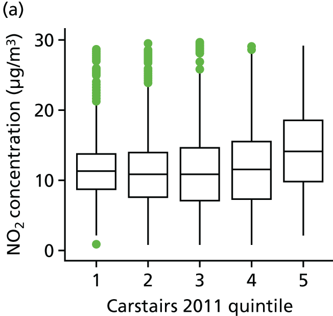
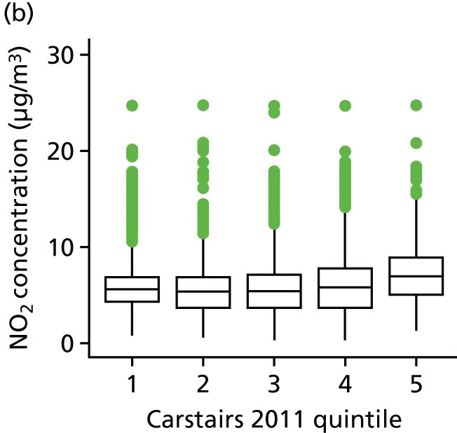
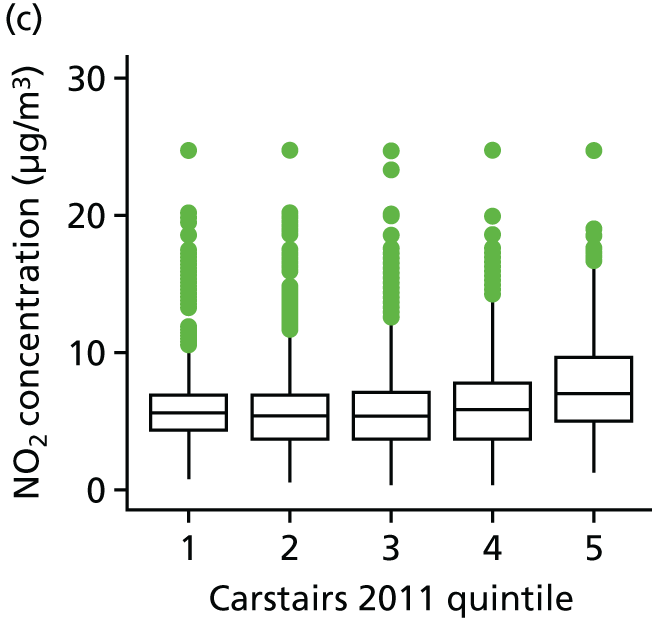

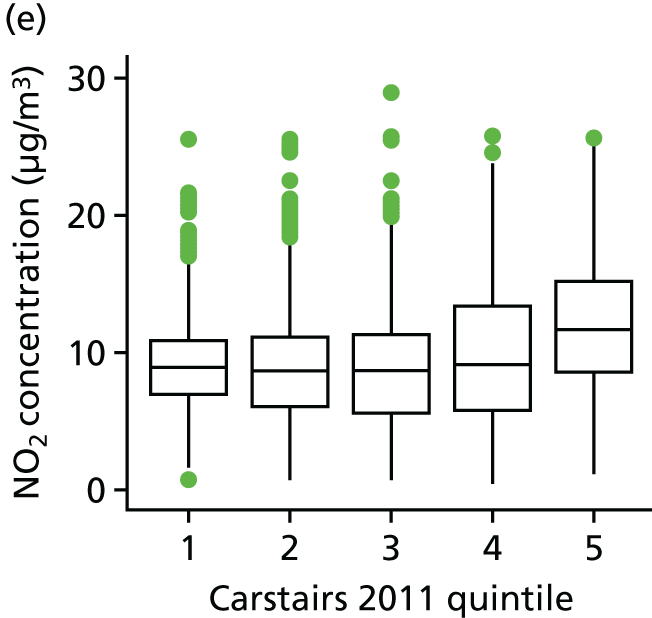
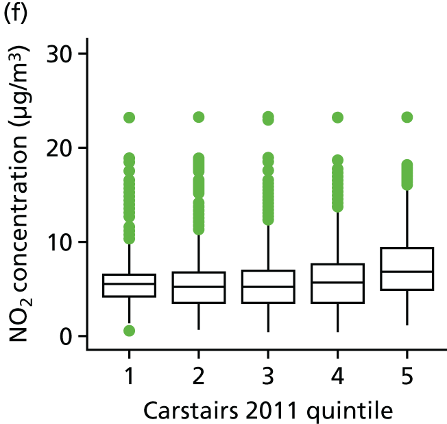
FIGURE 49.
Box-and-whisker plots showing distribution of ward 2011-level NO2 concentrations by Carstairs 2011 quintile at 2011 baseline and under different scenarios in London. (a) 2011; (b) 2035 baseline; (c) 2035 NRPO; (d) 2050 LGHG; (e) 2050 baseline; and (f) 2050 NRPO.
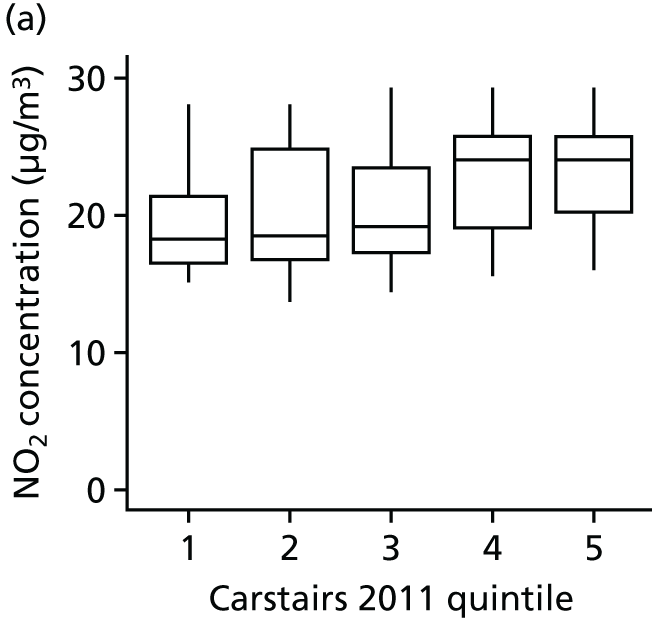
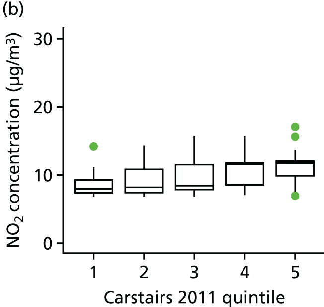
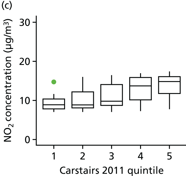
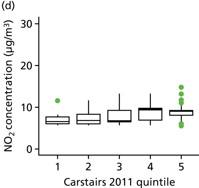
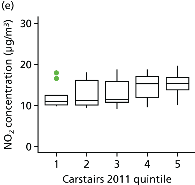
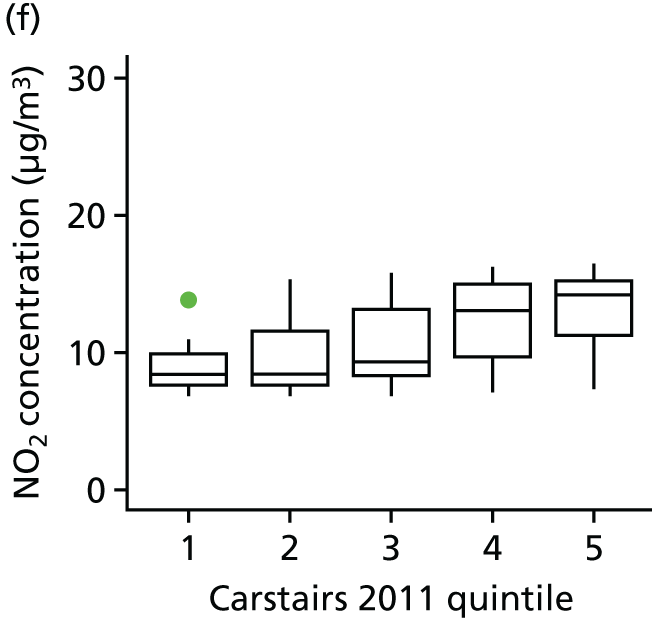
FIGURE 50.
Box-and-whisker plots showing distribution of ward 2011-level NO2 concentrations by Carstairs 2011 quintile at 2011 baseline and under different scenarios in Wales. (a) 2011; (b) 2035 baseline; (c) 2035 NRPO; (d) 2050 NRPO; (e) 2050 LGHG; and (f) 2050 baseline.
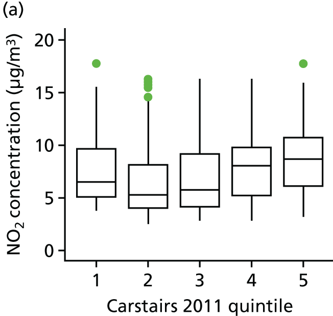
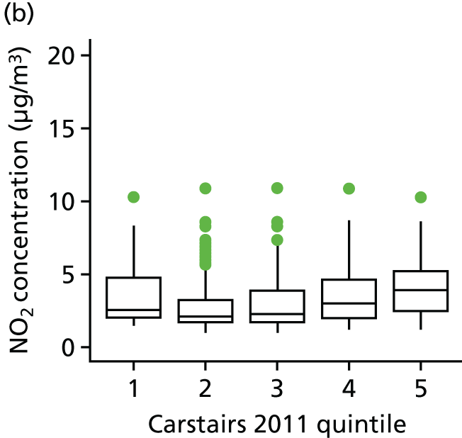
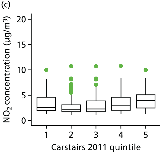
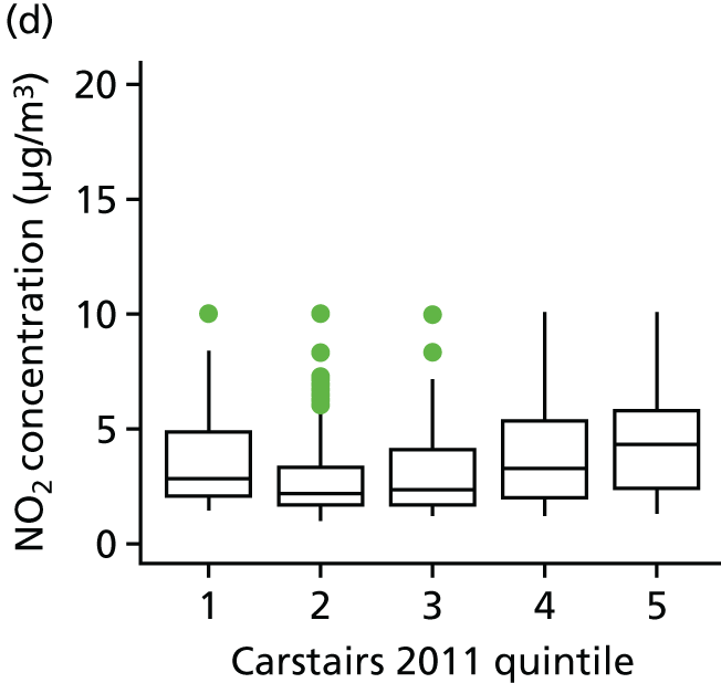
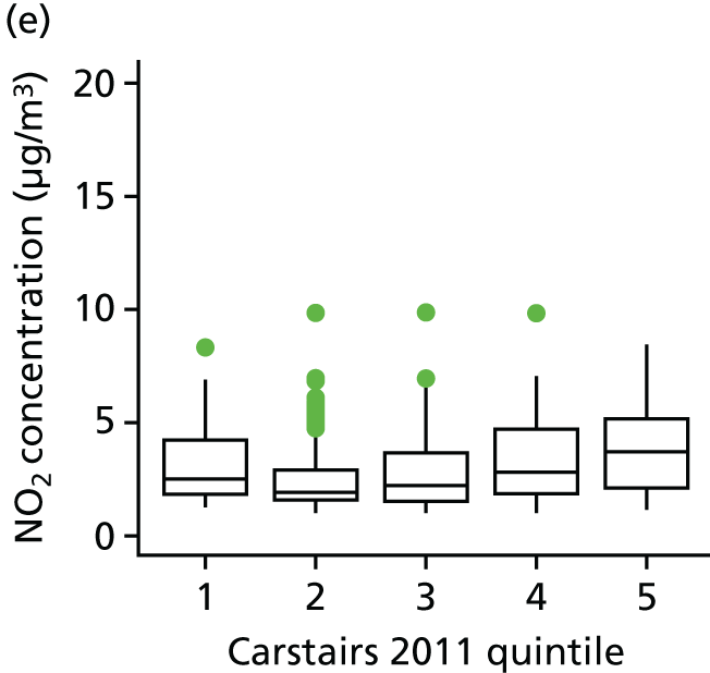
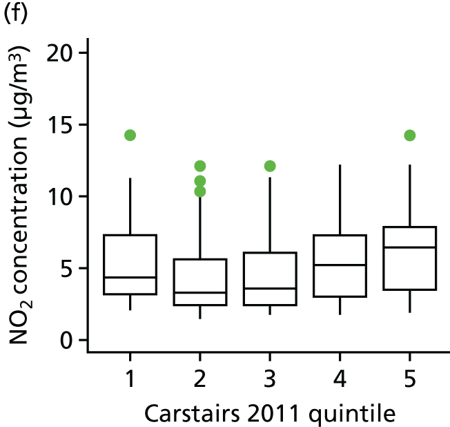
FIGURE 51.
Box-and-whisker plots showing distribution of ward 2011-level NO2 concentrations by Carstairs 2011 quintile at 2011 baseline and under different scenarios in Scotland. (a) 2011; (b) 2035 baseline; (c) 2035 NRPO; (d) 2050 LGHG; (e) 2050 baseline; and (f) 2050 NRPO. NA, not applicable.
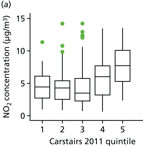
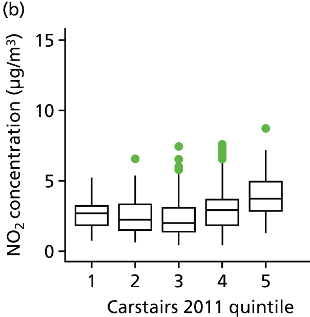
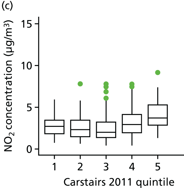
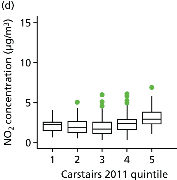
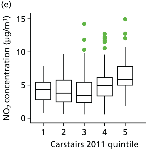
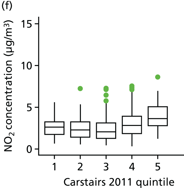
In GB, we observed stable mean NO2 concentrations for the first to fourth quintiles, but higher mean NO2 concentrations for the fifth quintile. In London, NO2 levels steadily increase from lowest to highest deprivation quintile. In Wales and Scotland, we observed more U- and J-shaped distributions, respectively, of NO2 concentrations with lowest concentrations in the middle deprivation quintiles. In all regions, however, wards in the lowest deprivation quintiles had the highest mean NO2 concentrations.
Discussion and conclusion
We analysed small area associations of air pollution exposures with ethnicity and socioeconomic deprivation for current and future projection scenarios. We observed differences in air pollution levels by subpopulations for all analysed pollutants and for each geographical area. Differences in exposure were most marked for NO2, as shown in Table 23 for ethnicity and Table 24 for socioeconomic deprivation. This is unsurprising as NO2 is predominantly a primary pollutant (i.e. its concentrations are less dependent on slow chemical reactions in the atmosphere and are hence highest near to sources, which, for virtually all areas of GB, are roads). Wards with higher proportions of non-white residence and higher deprivation are expected to be closer to roads and, therefore, have higher NO2 levels. Relative differences (i.e. ratios) in NO2 between white and non-white populations were much larger than the differences between the most and least deprived populations in GB and Wales in 2011, but slightly smaller in London. Relative differences between most and least deprived populations in 2011 were highest in Scotland, closely followed by London; relative differences in Wales were the smallest.
Ozone and PM2.5 show smaller differences. A significant fraction of PM2.5 in GB is made up of secondary aerosol formed over long periods (up to several days) from emissions in other parts of GB and in the rest of Europe. Spatial patterns of PM2.5 annual averages are therefore more homogeneous than for NO2. The relative differences between subpopulations are consequently smaller than for NO2.
Ozone is a purely secondary pollutant with a fairly homogeneous spatial distribution across the country, but with the added factor that it is destroyed by chemical reactions with fresh NOx emissions. Annual average O3 concentrations are, therefore, smaller in areas where NO2 is higher and levels are, hence, lower in areas closest to roads and in cities. This effect across the ward level is averaged out to some extent, so the differences between subpopulations are relatively small for all geographical areas and there is essentially no difference in annual mean O3 exposures across the country at the ward level.
The future scenarios all reduce the absolute values of the concentrations, with the exception of the NRPO scenario in 2035. This scenario includes a large increase in biomass, discussed above, and this is probably the reason why the concentrations are no lower than those in the baseline scenario. The LGHG scenario also has a similarly large increase in biomass and, although we did not model the 2035 LGHG scenario, the exposures for PM2.5 would be expected to be very similar to those of the NRPO scenario in 2035, as they are in 2050.
There is some indication that the future scenarios for NO2 reduce the differences between most and least deprived populations as measured by the ratios (apart from the high biomass 2035 NRPO and probably the 2035 LGHG scenarios). This is less clear for PM2.5, and there is even some indication that, in this case, the ratios increase.
For O3, all future scenarios show almost identical exposures across the indices for most and least deprived populations.
The plots in Figures 48–51 show that, despite the large decreases in NO2 concentrations, there are still differences in exposures across the deprivation quintiles. This is because, in the future scenarios, NO2 concentrations are still highest near roads despite the large reductions in road traffic emissions, as discussed in Chapter 6. The increase in exposure across the deprivation quintiles is steady in London, whereas in Scotland the lower quintiles are broadly similar in exposure with the highest quintile showing a marked increase. In Wales, the NO2 levels by quintiles show more of a U-shaped behaviour, with the least deprived classes having slightly higher exposures, although the most deprived wards show the highest exposures in all scenarios.
Overall, therefore, we conclude that all future scenarios reduce the absolute levels of pollution exposure in all deprivation quintiles across GB, except in those scenarios where there is a large increase in biomass burning. Differences in exposure between the most and least deprived populations remain in all future scenarios, most clearly for NO2, but are somewhat reduced. From the environmental inequality perspective, there appears to be little difference in NO2 exposure differentials between most and least deprived groups when comparing the baseline scenario, which does not meet the CCA target, and the NRPO scenario, which meets the target but with limited nuclear build. The NRPO scenario leads to a higher NOx emission than the LGHG scenario, which meets the CCA target with no constraint on nuclear build. In this latter scenario, for London at least, the differences in exposure between the most and least deprived populations look to be smaller than in the other two scenarios. The absolute differences for the LGHG scenario are 1.7 µg/m3, baseline 2.8 µg/m3 and NRPO 4.1 µg/m3.
Chapter 9 Economic valuation of the air quality impact on mortality
In undertaking a valuation in monetary terms of the mortality impact described in Chapter 8, we have used the methods set out in an earlier report from King’s College London on the health impact of air pollution in London. 101 This built on previous work by the study team for Defra and the Interdepartmental Group on Costs and Benefits within the UK government. The methods are therefore consistent with those used in government in the UK.
Methods
General approaches
It is first necessary to distinguish between different approaches for valuation of health impact as used in the disciplines of health economics, which is widely used already in the NHS (e.g. in guidance from the National Institute for Health and Care Excellence), and environmental economics, which is not, with preference here given to the latter.
In the context of health economics in the UK, impact is frequently valued in terms of quality-adjusted life-years (QALYs). A QALY score of 1 indicates a year of life in perfect health, whereas a score of 0 indicates death or a zero quality of life. There are various methods available for deriving QALYs. 149 One widely used approach for deriving QALYs for specific conditions is time trade-off analysis, which seeks to describe the preference that individuals have for improving their health. The trade-off takes the form of considering the amount of time that one would be willing to spend in perfect health as opposed to time spent with a reduced quality of life. Interviews are generally performed by trained medical staff. Subsequent analysis can then consider what is variously described as the cost-effectiveness or cost–utility of different treatment options, in terms of cost per QALY, in order to direct available resource towards the treatments that will prove most beneficial for the society served by the health system in question. This general approach is extensively used by the National Institute for Health and Care Excellence.
The approach taken here, however, is based on the discipline of environmental economics. 150 Environmental economics was developed partly in response to recognition of the externalities, or external costs, posed by various human activities. ‘Externalities’ are unforeseen effects that arise from action that benefits one party, generally to the detriment of others, when those effects are external or not considered in the decision-making process. Notable examples include the loss of utility from effects of air pollution arising from power generation or transport. The question faced by the economist in this situation is not how to allocate a defined amount of resource (the health service budget), but how much should be spent to mitigate externalities. This requires that health impact is monetised in order that the benefits of action can be compared directly with the costs in a benefit–cost analysis.
Several approaches have been taken to value mortality impact (the impact that dominates the assessment made in this report), although all seek to quantify public preference, demonstrating consistency in objective with the health economics work in deriving QALYs for various conditions. The methods used for valuing a death fall into three categories:
-
wage–risk studies, which consider the additional wage demanded of people working in risky occupations, providing an estimate of willingness to accept risk
-
consumer market studies that consider the willingness of individuals to pay for equipment that will reduce their risk of death [e.g. several studies were carried out on car safety equipment (air bags, etc.) before they were made mandatory]
-
contingent valuation surveys, in which individuals are asked for their willingness to pay (WTP) for treatments that will reduce the risk of a health impact of some kind, or of dying within ‘X’ years.
Early work in this field was affected by various biases. Considerable effort has been taken over the last three decades to identify these biases and refine contingent valuation approaches to reduce them, with some success.
In the context of health valuation, the underlying calculations are similar for whichever of the three methods just mentioned is used. In the case of the wage–risk studies, for example, it may be observed that construction workers operating at height will accept an additional risk of death annually of 1 in 1000 (0.001) for an additional wage of £1000. The value of statistical life (VSL) calculated from these figures would be £1000/0.001 – £1M. A review by the Organisation for Economic Co-operation and Development (OECD) gives an averaged VSL for EU member states of €3M. UK government, via the Department for Transport, adopts a value that is lower by about 40% of £1.56M. 151
Opinion is divided as to whether valuation of mortality should concern ‘deaths’ or ‘life-years lost’. The OECD is firmly committed to use of the VSL. 152 The UK government, through the Interdepartmental Group on Costs and Benefits, however, values mortality in terms of the loss of life expectancy expressed as the ‘value of a life-year’, taking a value of £36,379 in 2014 prices. The basic approach to quantification, however, is the same, with values elicited against a change in the risk of a health outcome, in this case the loss of a life-year. The large difference between the unit values for VSL and value of a life-year is partly mitigated in subsequent analysis by the number of life-years lost being about 10 times higher than the number of deaths. However, the UK government position generates estimates of air pollution damage that are significantly lower than estimates made using the OECD position. Given that the UK government position is followed here, the results should be considered to be at the conservative end of plausible ranges.
Similar calculations can be made to assess the WTP to avoid ill health more generally, such as development of respiratory or cardiovascular disease. The total impact for morbidity has a number of elements:
-
WTP to avoid lost utility (being well and enjoying the opportunities that good health offers)
-
the costs of health care
-
costs to the marketed economy through lost productivity.
Costs have been defined for a variety of end points of relevance to air pollution in analysis for UK government and also for other bodies, such as the European Commission. 153,154
Adopted values, discounting and uplift
The values of most relevance concern acute and chronic mortality, as these have been shown by numerous studies to dominate the cost–benefit analysis. The value of a lost year of life to chronic exposure as applied in the current analysis is £36,379, assuming that it reflects the loss of a year of life in ‘normal health’ taken from the guidance issued by Defra. 155
It is important to factor the time at which impacts occur into the analysis for two reasons. The first is that values should be uplifted for future years to capture the likely effect of (anticipated) growth in incomes on WTP for health protection. The second, opposing, effect concerns the need to discount future values on the basis that money or goods are more valuable now than at some point in the future. There are several reasons for this. One is that resource available now can be used to increase the availability of resource in the future. An obvious example concerns investment in infrastructure projects that facilitate economic development. Along similar lines, investment in health research may lead to the development of cures or treatments for illnesses in the future. Further information can be found in Guidance from Her Majesty’s Treasury in the ‘Green Book’. 156
The ‘Green Book’ recommends the use of declining discount rates for effects quantified over prolonged periods. However, the impact of using declining discount rates in line with Her Majesty’s Treasury recommendation, rather than constant discount rates, will be minimal as these rates apply only after 30 years have passed, by which time values are reduced by two-thirds. The impact of the declining rates will clearly increase over time, though the rate of decline is so slight that it will still make little difference (Table 25).
| Period of years | Discount rate (%) |
|---|---|
| 0–30 | 3.5 |
| 31–75 | 3.0 |
| 76–125 | 2.5 |
| 126–200 | 2.0 |
| 201–300 | 1.5 |
| 301+ | 1.0 |
The government guidance157 recommends that future values should be uplifted at 2% per annum; as incomes rise it is to be expected that WTP to avoid risks also rises. However, it is unclear whether or not the uplift of 2% is still appropriate. It is notable that the guidance was first developed before the economic crash of 2008 and so does not account for any change in growth since that time. However, the present analysis is based on a long time frame, so short-term perturbations to growth seem likely to be factored out in the longer term.
In conclusion, the method defined in the earlier King’s College London report,101 with respect to discounting and the uplift of future values, is in line with UK government guidance and hence should be considered appropriate here. There are reasons for adopting alternative positions on some aspects of the analysis, which could be adopted for sensitivity analysis.
Inequality is not factored explicitly into the economic analysis, beyond the acceptance of a national average estimate for mortality valuation (in other words, the values of disadvantaged groups are not down rated to reflect a likely lower WTP linked to reduced ability to pay).
Results
Under the baseline scenario, the overall magnitude of benefits equates to an annual cost of between £24B and £28B, depending on whether or not a threshold is adopted for assessment of effects quantified against NO2 exposure. Of this, roughly two-thirds of the impact is attributable to quantification against PM2.5 exposure (Table 26). To put these figures into some context, they are equivalent to 1.5% of current UK gross domestic product (GDP) under the baseline scenario. Of course, personal utility, as measured using the WTP paradigm for health, is not captured by GDP: this should be seen as a deficiency in the extent to which GDP describes wealth, rather than an indication that these monetised benefits are in some sense inferior or not truly a part of the national economy. 152
| Country/region | Scenario | ||
|---|---|---|---|
| PM2.5 | NO2 | NO2 with threshold | |
| England | 16,453 | 9234 | 5746 |
| Scotland | 856 | 480 | 170 |
| Wales | 705 | 314 | 136 |
| GB | 18,015 | 10,027 | 6052 |
Total annual monetised impact for each scenario is shown in Figure 52. It should be stressed here that combining the impact for PM2.5 and NO2 is performed here for illustrative purposes and is likely to represent an upper bound to the valuation. The issues around the role of NO2 in affecting health vis-à-vis PM2.5 have been discussed in Chapter 8, and the possible overlap in effects from the two pollutants has been partially accounted for in the CRFs, on the basis of the most recent advice available from COMEAP at the time of this study.
FIGURE 52.
Total monetised impact, £M/year, under each scenario for PM2.5 and NO2 (no threshold) combined (this is illustrative, see Results).
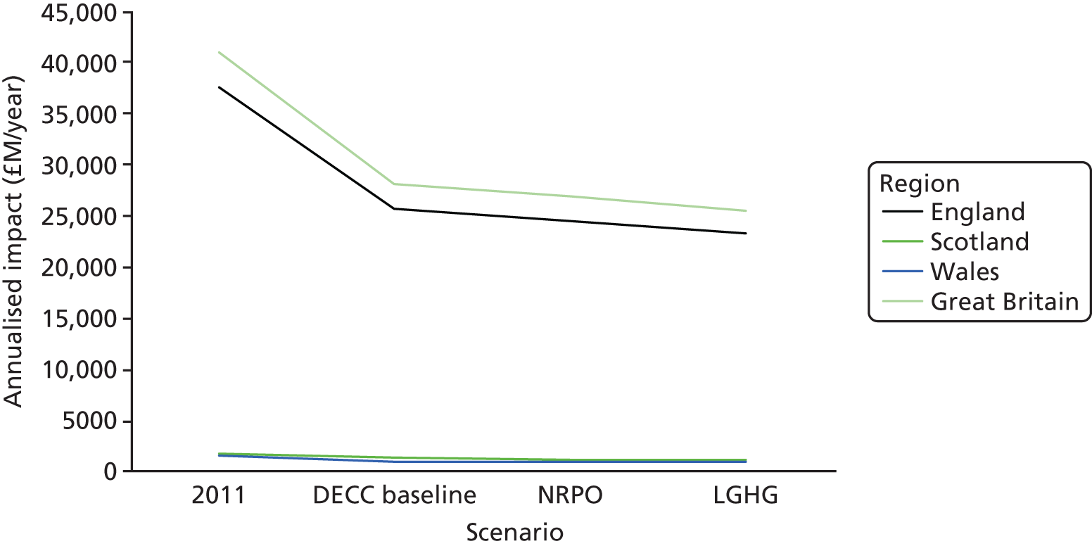
The figure first demonstrates the extent to which impact in England dominates the assessment. This domination is largely a consequence of the difference in population relative to Scotland and Wales, although higher pollutant levels, particularly in London and south-east England, also play a role.
The figure also demonstrates the decline in impact relative to the situation had 2011 conditions persisted. Most of the forecast benefit is attributable to the baseline rather than the NRPO or LGHG scenarios.
Table 27 breaks down the benefits for the LGHG scenario relative to the baseline. Table 27 shows negative benefit (increased impact) for assessment relative to PM2.5, through increased use of biomass for combustion. Benefits expressed against NO2 exposure outweigh these effects related to PM2.5 sufficient to generate an overall benefit for the LGHG scenario relative to the baseline of > £3B/year, equivalent to 0.2% of GDP, although this may be an overestimate. There is little difference between benefits regardless of whether a threshold is applied to NO2 exposure, indicating that by far the greater share of exposure reduction under the scenario occurs in locations that exceed threshold.
| Country/region | Scenario | ||
|---|---|---|---|
| PM2.5 | NO2 | NO2 with threshold | |
| England | –756 | 3103 | 2999 |
| Scotland | –2 | 149 | 98 |
| Wales | –82 | 85 | 66 |
| GB | –839 | 3336 | 3163 |
Discussion
The results demonstrate that the economic impact of air pollution on health is substantial, equivalent to around 1.5% of GDP (accepting that GDP is an imperfect measure of ‘wealth’, as it considers only the ‘productive’ economy and ignores goods such as health and well-being). These results are broadly consistent with those generated in other assessments of air quality impact.
The results across different scenarios, and the comparison with 2011 conditions, show that the policy scenarios make a smaller difference to the benefits of improving air quality than policies already accounted for in the baseline scenario (as shown by the difference between the benefits of baseline relative to 2011, and the NRPO and LGHG scenarios relative to the baseline). Given that certain of the measures in place in the baseline scenario are designed specifically to improve air quality, this is not surprising, as it leaves reduced scope for future improvements. Given that results highlight that there remains a substantial level of impact beyond NRPO and LGHG, it is appropriate to ask whether or not the climate policies could be better targeted on air quality: the most efficient approach for society will be derived from analysis that takes all impact of climate policies, including the cobenefits and trade-offs of climate actions, as well as direct climate-related benefits.
There are several methodological issues that affect the magnitude of economic estimates. The following examples provide illustration of issues that affect the results in different directions:
-
The valuations used in the UK are based on a limited literature and ignore the international literature (e.g. the OECD, 2012 meta-analysis152). Inclusion of studies from elsewhere could increase the valuations significantly. There is very little evidence to support the adoption of values lower than those used in the UK for the UK population.
-
The 2% uplift is based on an assumed growth in WTP in line with growth in incomes. This in turn implies an elasticity of 1. In relation to mortality valuation, OECD152 recommends an elasticity of 0.8, which would reduce estimated values in the future compared with the current assumption. OECD also recommends use of an even lower elasticity, 0.4, in line with the recommendations of US EPA.
Overall, it is considered here that there is more bias towards potential underestimation of economic impact than to overestimation, given the size of the difference between mortality valuations accepted by UK government and the wider valuation literature. Although different assumptions would affect the magnitude of results, they would not affect the relationship between the scenarios. They would, however, obviously affect the economic appraisal of abatement measures.
Chapter 10 Discussion and conclusions
Scientific conclusions
Scenario emissions
The two ‘CCA-compliant’ scenarios, NRPO and LGHG, had a high proportion of energy generated through biomass use with a large increase in PM2.5 emissions of approximately 50%, compared with 2011, and peaking in 2035. Although biomass use was projected to decrease again by 2050, primary PM2.5 emissions in 2050 were still marginally higher than 2011 levels. The baseline and reference scenarios, which did not meet the CCA target, had lower levels of wood burning.
Both the LGHG and the NRPO had a high degree of switching from petrol and diesel fuels to electric, hybrid and alternatively fuelled vehicles in the UK road transport fleet, leading to reductions of around 90% from transport sector NOx emissions in all scenarios except the baseline. The baseline scenario had higher gas and biomass consumption in CHP plants compared with other scenarios, as well as no obligation to meet the CCA target, and this lead to increased NO2 exposure. In the transportation sector, despite the exhaust emission reductions, the UKTM projections show large increases in traffic activity with car and heavy goods vehicle kilometres projected to increase by roughly 50% in all the scenarios and vans by a factor of about 2. This leads to a pro-rata increase in PM emissions from brake and tyre wear and resuspension of road dust, although these are uncertain as we have assumed in future that the emissions factors will remain at current levels. Consequently, non-exhaust emissions could be the dominant source of primary PM from vehicles in future, increasing PM10 by about 15% compared with 2011 in the NRPO scenario, for example. This is more of an issue for PM10, as the non-exhaust emissions are coarser in size.
Pollutant concentrations
Annual mean concentrations of NO2 are projected to decrease by about 60% in the LGHG scenario and by ≈50% in the NRPO scenario across the whole of GB and in London, but only by ≈20% across GB and ≈42% in London in the baseline scenario.
Annual mean PM2.5 concentrations are also projected to fall by around 40% in the top 25% of grid squares, but by only ≈25% in the highest areas. However, concentrations of primary PM2.5 are projected to increase in 2035 in the NRPO and LGHG scenarios, by around 30–60% in the more polluted grid squares, as a result of the increase in biomass use. By 2050, in those two scenarios, levels are only slightly lower than 2011 values and in the highest grid square are very similar to 2011 concentrations. If this amount of primary PM2.5 were to be removed, by avoiding the high use of biomass, total PM2.5 concentrations could fall even further than projected, down by ≈50% in the highest areas compared with ≈25% reduction with the increased biomass use.
Total PM10 concentrations are projected to increase in 2035 in many areas of the UK in both the LGHG and NRPO scenarios, despite the reduction in secondary PM precursors, because of the increased use of biomass and the increased non-exhaust emissions from transport. PM10 levels decrease again by 2050, but remain only about 15% smaller than 2011 in the more polluted areas of GB. This is a small reduction and is not larger because of the increasing contribution from non-exhaust emissions. This is of concern as these emissions are potentially toxic.
The reductions in NOx emissions result in increasing annual average O3 concentrations in urban areas, leading to higher exposures using the metric recommended by COMEAP for short-term impact on mortality. In contrast, all scenarios show reductions in the metric suggested by the WHO for long-term O3 exposure impact on mortality.
Both O3 and NO2 are strong oxidising agents and can play a role in oxidative stress in the human body. This can be quantified through the use of the metric Ox or oxidant (Ox = O3 + NO2), which has been shown to be associated with adverse health outcomes. Annual average levels are projected to remain virtually constant to 2050. The significance of this for health is that the balance of Ox will shift to O3 as NO2 reduces; the former is the more powerful Ox so that the oxidising power of the urban atmosphere in the UK will increase with potentially increased adverse health effects, assuming that the global background of O3 remains broadly constant.
Health impact
We have calculated impact arising from long-term exposures to the pollutants PM2.5, NO2 and O3, on mortality, using a life table approach to calculate the loss of life-years in each of the scenarios. This now incorporates birth projections, projected improvements in mortality rates and mortality rates at local authority level. The two scenarios which achieve the CCA target result in more life-years lost from long-term exposures to PM2.5 beyond the carbon policies already in place and the levels of PM2.5 still result in a loss of life expectancy from birth in 2011 of around 4 months. This is an important opportunity lost and arises from the large increase in biomass use peaking in 2035. Our estimates suggest that in the more highly polluted areas of GB, total PM2.5 concentrations could reduce by as much as 50% without the biomass contribution.
There is currently some uncertainty over the role of NO2 vis-à-vis PM2.5, but using the CRFs currently suggested by COMEAP, reduced long-term exposures to NO2 lead to more life-years saved and an improvement of 2 months in loss of life expectancy from birth in 2011 in the ‘CCA-compliant’ scenarios compared with the baseline scenario, with the largest benefits arising from the most ambitious scenario LGHG.
Evidence for impact on mortality of long-term exposures to O3 is increasing, although using the quantification recommended by WHO we estimate life-years lost from this exposure to be smaller by factors of ≈6 and ≈3–4, than those from PM2.5 and from NO2, respectively, if no threshold is assumed for NO2. However, the short-term O3 exposure metric recommended by COMEAP suggests the number of DBF in a year could be around 22,000 compared with 29,000 from long-term PM2.5 exposures.
However, it should be noted that the distinction between effects attributable to NO2 and those attributable to PM2.5 and the issue of how if, at all, one might add the effects of both pollutants is still a matter of some uncertainty. COMEAP is currently in the process of preparing a report on this subject, unpublished at the time of writing.
The issue of a no-effects threshold is also very important on quantifying the impact of O3 concentrations. The long-term exposure metric recommended by WHO in the HRAPIE project95 as a sensitivity study included a threshold of 35 p.p.b. or 70 µg/m3 and resulted in an impact on life-years lost much smaller than those of PM2.5 and NO2. However, the short-term exposure metric recommended by COMEAP did not incorporate a threshold, and a rough calculation suggests that the impact from this metric of O3 concentrations could lead to the number of DBF of a similar order to that for PM2.5, approximately 20,000 from O3 exposure compared with 29,000 from PM2.5.
We also investigated the effect of the changing concentrations on exposures in different socioeconomic classes. We observed differences in air pollution levels in subpopulations for all analysed pollutants and for each geographical area. Differences in exposure were most marked for NO2 for ethnicity and for socioeconomic deprivation. Wards with higher proportions of non-white residence and higher deprivation are expected to be closer to roads and, therefore, exposed to these higher NO2 levels. The ratios of exposures in white and non-white populations were much larger than those for the most deprived populations compared with least deprived populations in GB and Wales, but slightly smaller in London. Relative differences between most and least deprived populations were highest in Scotland, closely followed by London; relative differences in Wales were the smallest.
All future scenarios reduced the absolute levels of pollution exposure in all deprivation quintiles across GB, except in those cases in which there is a large increase in biomass burning. Differences in exposure between the most and least deprived populations remain in all scenarios, most clearly for NO2, in which there is little difference between the baseline scenario and the NRPO scenario.
Limitations of the research
Although we have presented an advanced and detailed modelling study of the air pollution impact on health from climate policies, there are inevitable limitations to the work. We used the complex UKTM energy model as this represents a much more detailed method of generating energy scenarios than our original proposal. Because of this we were able to run only a limited number of scenarios. A wider range of pathways to the CCA would have potentially quantified a larger degree of health improvements in future years. The complexity of the UKTM model and the system we have built requires significant computer resources so that it is impracticable to undertake a range of sensitivity analyses around the economic parameters and energy and transport futures in the UKTM model.
Air quality modelling is always limited by several factors, the most important of which is the accuracy of the emissions inventory input. We improved the existing inventories using the most up-to-date information, but there are inevitably limitations to this knowledge. Equally, our understanding of the mechanisms of particle formation is developing continuously and, although we have used the best available chemical/physical mechanism of particle formation, there are still uncertainties involved here.
The health impact calculations are limited by the uncertainty in the numerical coefficients relating health outcomes to air pollutant concentrations, although to a degree we have allowed for this via the confidence intervals incorporated in the epidemiological studies. An important limitation is the extent to which the science supports an independent effect of NO2 compared with PM2.5 and the degree of overlap between the two pollutants in the association with adverse health outcomes. The review of the evidence by COMEAP, due to be published near the time of writing, had not appeared as this report was finalised.
Although improving the modelling scale down to 20 m in urban areas is an important advance in picking up exposure contrasts (particularly close to roads), the health impact methodology used is not, at this stage, able to take full advantage of this. In order to be able to use routinely available statistics on population and mortality by age group, concentrations were averaged up to ward level. Depending on how small-scale variations in population and mortality line up with variations in pollutant concentrations (particularly NO2), results could differ if finer-scale inputs were used for population and mortality as well as concentration.
Uncertainties
Uncertainties in emissions and air quality modelling
The energy scenario modelling represents a series of hypothetical futures, and, if we were trying to predict actual future energy use in a forecasting sense, we would have needed to explore the uncertainties around the economic forecasts, for example. However, in the sense that we have used the projections – in a ‘what if?’ sense – then these uncertainties become less relevant.
The development of a new energy and air quality model has been a significant undertaking and represents an important step forward as a policy development tool. The inputs to the model system are numerous and the uncertainties are difficult to test in a comprehensive way, and, although we have started to look at methods to test the CMAQ model uncertainties for O3 predictions, these methods have not been used in the present work.
In lieu of a detailed uncertainty analysis we have provided results of a model evaluation exercise across GB using 80 measurement sites. Using the criteria in a recent model evaluation exercise, we have confidence that the combination of the WRF meteorological model, emissions and CMAQ/ADMS air pollution models is able to reproduce 2011 and 2012 concentrations of NOX, NO2, O3, PM10 and PM2.5 at spatial scales, from 10 km across the UK, down to 20-m scale in urban areas. Furthermore, comparison with PM component measurements (nitrate, sulphate, OA, etc.) from the London 2012 ClearfLo campaign show good agreement, which is encouraging both from a model chemistry point of view, but also because it supports the introduction of new emissions to the model, such as domestic wood burning, cooking and diesel IVOCs. The UKTM model has also been evaluated against 2010 energy statistics and WRF assessed against 169 UK Met Office measurement sites.
There is uncertainty in future emissions predictions over whether we use energy-related activity data from the UKTM model or emissions factor assumptions, although for the latter we have used UK NAEI 2030 emission factors as far as possible.
Specific examples include uncertainties in our understanding of PM10 non-exhaust emissions, which are assumed to increase pro rata with vehicle kilometres to 2050. This assumption may change as some private cars become lighter, are fitted with lower rolling resistant tyres and use regenerative braking, whereas delivery vehicles become heavier, and as all vehicles are subject to increased city congestion and there are ongoing changes to the materials used in brakes and tyre manufacture. Without regulation of these sources future predictions should be considered with caution.
Furthermore, the treatment of domestic wood burning emissions makes assumptions regarding the mix of wood burning appliances resulting in a 19% reduction in PM emissions per kilogram of wood burnt, as a result of the introduction of stoves complying with emission limits in the Ecodesign Directive (53% reduction in PM emissions compared with existing wood burners) and large pelletised domestic appliances (93% reduction in PM emissions compared with existing wood burners) in the UK appliance stock. Another important uncertainty is the location of CHP stations, which we have assumed is the same as existing UK locations for this source (i.e. in northern UK cities). Although this is not unreasonable, the introduction of CHP is already happening in other cities such as London and, although not likely to change the total emissions in our model, will possibly spread the impact away more widely than we have assumed.
Finally, although there will always be uncertainty in future predictions, the project aims were to provide alternative future scenarios, pointing out the potential for undesirable air pollution impacts within climate change policy and accepting that a large range of outcomes are possible.
Uncertainties in health and inequalities
Calculations were done using the confidence intervals (or plausibility intervals in the case of PM2.5) to give one indication of a range of possible answers. For PM2.5 this gave a range for the life-years lost or gained from one-sixth to twice the result for the central estimate. This was in line with the range for the originating CRF. The proportion relative to the central estimate varied very slightly – because of the non-linearities in the calculations. This range is not that for a 95% confidence interval. The original COMEAP recommendations included wider uncertainties than just those relating to statistical sampling. In addition, uncertainties in other inputs are not included. The range for the differences between scenarios was derived by subtracting the lower ends of the ranges for each scenario from each other – this probably overestimates the range. The impact of the spatial scale of the modelling was investigated, but not other issues so far. Some inputs are well established (e.g. population and deaths data), but, even in that case, assumptions are required, for example inferring distribution by age at small local areas from distributions at a wider geographical scale. The uncertainties in the modelling data have been discussed above but have not, so far, been propagated to the health impact calculations. In principle, this could be done, but would involve a much larger resource than was available in this project. There are a variety of versions of mortality rate improvement projections and birth projections – we have used only the central ones. Migration was not included and it is very unclear at present in which direction this will go.
Many of the same issues apply to the calculations for NO2 (with and without a cut-off point). In terms of the 95% confidence interval of the CRFs, the results varied from 41%/42% of the central estimate to 1.6 times the central estimate. This only represents one aspect of the uncertainty. Results can be sensitive to the choice of cut-off point.
As described in Chapter 8, we assumed that deprivation and ethnicity patterns at the small area level observed in 2011 are representative for the years 2035 and 2050. This assumption is based on studies which have shown that, in particular, deprivation patterns are fairly stable over time. We used this approach because no information on future deprivation or ethnicity patterns is available that far into the future. Uncertainties associated with such future sociodemographic prediction would be expected to not be dissimilar to those associated with our approach.
Inevitably, assumptions have to be made when projecting into the future. Inclusion of projected mortality improvements and birth projections improved this, compared with assuming baseline mortality rates and births remaining the same. However, these projections themselves are uncertain. In addition, we did not include projections of migration at this stage.
The project’s contribution to advances in knowledge
This project has, for the first time in the UK, delivered a sophisticated tool to enable the explicit calculation of public health impact arising from future energy strategies in GB using a state-of-the-art air quality model with an energy systems model used to inform government policy on greenhouse gas mitigation. This represents a major improvement over previous approaches to the impact of greenhouse gas emissions. Our work has established a method of calculating public health impact of air pollution resulting from climate policies through the full ‘impact pathway’ approach rather than the cruder, more approximate, ‘damage cost’ approach. The latter approach has been used to date by government in the UK to appraise climate policies; it relies on simply assigning a monetary value to a unit of air pollution emission. Consequently, there is no explicit calculation of pollution concentrations in the air, or of the impact on mortality and morbidity. Our system now allows that to be done in a linked system beginning with the economic model of the British energy system, through a sophisticated air quality model to a detailed life table model for calculating impact on health, on exposures in socioeconomic classes and for calculating economic impact. Moreover, the system we have developed allows this impact to be calculated at the finest spatial resolution yet achieved in GB, in which we model the rural areas at 10 km and major urban centres at 2 km or as fine as 20 m.
The science of air quality and of PM has continued to evolve during the life of the project. During the study it was necessary for us to incorporate emerging research on the sources of PM from cooking sources that were not previously included in emission inventories in GB. We have also built on King’s College London’s expertise in understanding the contribution of wood (biomass) burning to air quality to improve the inventory of emissions from this source. We were also able to enhance our model to treat the major British cities at a spatial resolution of 20 m, where previously we had been able to do this only for London. We have evaluated this improved air quality model and shown it to behave well against accepted criteria.
During the course of the project, we formed a collaboration with the Institute for Sustainable Resources at UCL to allow us to link the UKTM energy systems model with our air quality model and our health impact capability. This formed a major advance and the link now establishes a credible system to assess the impact of energy futures and climate policies in GB.
Discussion
There are several important policy messages which arise from this project. The CCA target, in principle, offers a great opportunity to make very large reductions in air pollution emissions as the UK energy system is decarbonised. However, the PM2.5 emissions from the large increases in residential and CHP biomass use and the increase in non-exhaust PM emissions from transport in the two CCA-compliant scenarios we have studie mean that PM2.5 and PM10 concentrations do not fall as much as they would otherwise have done without the biomass use. This increase in biomass use has resulted in the finding that the CCA-compliant scenarios result in more life-years lost than the baseline scenario which incorporates no further climate action beyond that already in place.
Solutions to improve air quality impact on health could include measures to discourage the use of biomass in small installations, or to increase the stringency of the emission limits in the Ecodesign Directive. The related study by Lott et al. ,33 using the damage cost approach, carried out a calculation including damage costs for biomass use to attempt to account for the public health impact. This succeeded in reducing the use of biomass in the hypothetical calculation. In reality, measures to discourage biomass use would probably be best delivered through revisions to the renewable heat incentive. In terms of improving air quality and minimising the impact on public health, wood burning, if it were to be used at all, would be best deployed in large, efficient power stations rather than small-scale domestic or CHP use. Fiscal measures in the renewable heat incentive to encourage this shift would have benefits to public health without necessarily compromising the achievement of the CCA target.
Non-exhaust emissions of PM10, and to a lesser extent PM2.5, are projected to increase significantly by 2050 as traffic activity increases. The precise agents in tyre and brake wear and resuspended dust responsible for the potential toxicity of these emissions are, as yet, unclear, so reformulation of these products would need to await more clarification from toxicological research. However, in the meantime, the obvious solution to ameliorate potential impact from all emissions from road transport here would be to discourage traffic use, particularly in urban centres.
On the positive side, electrification of the road transport fleet results in large reductions in the potential adverse impact on health from NO2 and potential compliance with legal standards. This will also have benefits for PM concentrations and will, to a limited degree, offset the impact of any continued increase in biomass use.
The use of economic appraisal provides a mechanism for assessing the efficacy of measures for further action, permitting direct comparison of costs and benefits of measures, and enabling collation of a variety of different types of effect. As shown above, economic damage associated with air pollution in the UK is substantial and will remain so over the period covered by the scenarios considered here. It is noted that the UK approaches to valuation appear highly conservative compared with assumptions followed in the wider international literature.
Further research with the linked UKTM and our air quality model, CMAQ-Urban, could investigate other possible scenarios which achieve the CCA target and which could minimise the problem with residential and CHP biomass use and the impact of non-exhaust road transport emissions.
Recommendations for future research
The system we have developed links together a sophisticated energy system model – used by government in the UK – with a detailed chemical–transport model for air quality, health impact calculations and assessments of exposures and impacts in different socioeconomic classes. It also allows the monetary valuation of this impact on health. Because of the complexity of the system we have been able to run only a small number of scenarios and, although we have demonstrated some significant issues for future climate change mitigation measures, there is still scope to address optimal pathways for attaining the CCA target by minimising the impact on air quality and public health.
The work has shown that trends in different fractions of the atmospheric particle mix may be different in future. Primary particles (containing known carcinogens) may increase, whereas secondary particles may decrease. This highlights the importance of studies to elucidate the differential toxicity of different particle fractions.
The work has shown that, with increased penetration of ultra-low and zero-emissions road vehicles, concentrations of NO2 will decrease by large amounts. The precise role of NO2, compared with that of PM2.5 and other pollutants, in affecting human health is still uncertain. More clarity is needed here before any health benefits from reductions in NO2 can be confidently quantified.
The effects of long-term exposure to air pollution on mortality generally dominate cost–benefit analysis, but a full investigation of the health impact would involve quantifying the potential effects on a wider range of health outcomes. In addition, further sensitivity analyses on the data inputs and assumptions regarding CRFs (e.g. effect modification) would be helpful. There is a need to explore how using population and mortality inputs at a finer geographical scale affects the result. More meta-analyses of epidemiological studies on PM2.5 and NO2 will also be useful.
Acknowledgements
The authors would like to thank the National Institute for Health Research for funding this work under project number 11/3005/13.
In addition, authors would like to thank Dr Gregor Stewart (King’s College London) for help with the emission inventory.
Contributions of authors
Martin L Williams (Professor of Air Quality Research, King’s College London) was responsible for the concept and design of the study, advice and direction of scenario building and modelling, and overall production of the report.
Sean Beevers (Senior Lecturer, Air Quality Modelling, King’s College London) was responsible for the management and direction of air quality modelling, transforming UKTM output to give air pollutant emissions and contributing to report writing.
Nutthida Kitwiroon (Senior Air Pollution Scientist) was responsible for setting up CMAQ air quality model runs and running the model, plotting and analysing the air quality model results.
David Dajnak (Principal Air Quality Scientist, King’s College London) was responsible for health impact assessment and life table calculations.
Heather Walton (Senior Lecturer, King’s College London) was responsible for the direction of, and contributing to, the health impact assessment, life table calculations and contributing to report writing.
Melissa C Lott (Doctoral Researcher, UCL) was responsible for UKTM scenario design and production.
Steve Pye (UCL) was responsible for UKTM scenario design and production.
Daniela Fecht (Imperial College London) was responsible for the social deprivation analysis.
Mireille B Toledano (Imperial College London) provided advice on the design of the social deprivation analysis.
Mike Holland (Economic Consultant, Ecometrics, Research and Consulting) provided advice on economic impact.
Publication
Williams ML, Lott MC, Kitwiroon N, Dajnak D, Walton H, Holland M, et al. The Lancet Countdown on health benefits from the UK Climate Change Act: a modelling study for Great Britain. Lancet Planet Health 2018;2:e202–13.
Data sharing statement
Data used, or referred to, in this report may be obtained by contacting the corresponding author (Professor Martin Williams, King’s College London).
Disclaimers
This report presents independent research funded by the National Institute for Health Research (NIHR). The views and opinions expressed by authors in this publication are those of the authors and do not necessarily reflect those of the NHS, the NIHR, NETSCC, the PHR programme or the Department of Health and Social Care. If there are verbatim quotations included in this publication the views and opinions expressed by the interviewees are those of the interviewees and do not necessarily reflect those of the authors, those of the NHS, the NIHR, NETSCC, the PHR programme or the Department of Health and Social Care.
References
- Vardoulakis S, Heaviside C. Health Effects of Climate Change in the UK 2012. Current Evidence, Recommendations and Research Gaps 2012. www.gov.uk/government/uploads/system/uploads/attachment_data/file/371103/Health_Effects_of_Climate_Change_in_the_UK_2012_V13_with_cover_accessible.pdf (accessed 6 December 2016).
- Department for Environment, Food & Rural Affairs . Air Pollution in a Changing Climate 2010. www.defra.gov.uk/publications/2011/04/13/pb13378-air-pollution/ (accessed 6 December 2016).
- Williams ML. Tackling climate change: what is the impact on air pollution?. Carbon Manag 2012;3:511-19. https://doi.org/10.4155/cmt.12.49.
- Hendriks C, Forsell N, Kiesewetter G, Schaap M, Schopp W. Ozone concentrations and damage for realistic future European climate and air quality scenarios. Atmos Environ 2016;144:208-19. https://doi.org/10.1016/j.atmosenv.2016.08.026.
- Watson L, Lacressonniere G, Gauss M, Engardt M, Andersson C, Josse B, et al. Impact of emissions and +2C climate change upon future ozone and nitrogen dioxide over Europe. Atmos Environ 2016;142:271-85. https://doi.org/10.1016/j.atmosenv.2016.07.051.
- Colette A, Bessagnet B, Vautard R, Szopa S, Rao ST, Schucht S, et al. European atmosphere in 2050, a regional air quality and climate perspective under CMIP5 scenarios. Atmos Chem Phys 2013;13:7451-71. https://doi.org/10.5194/acp-13-7451-2013.
- Braspenning Radu O, van den Berg M, Klimont Z, Deetman S, Janssens-Maenhout G, Muntean M, et al. Exploring synergies between climate and air quality policies using long-term global and regional emission scenarios. Atmos Environ 2016;140:577-91. https://doi.org/10.1016/j.atmosenv.2016.05.021.
- Liu Q, Lam KS, Jiang F, Wang TJ, Xie M, Zhuang BL, et al. A numerical study of the impact of climate and emission changes on surface ozone over South China in autumn time in 2000–2050. Atmos Environ 2013;76:227-37. https://doi.org/10.1016/j.atmosenv.2013.01.030.
- Wang Y, Shen L, Wu S, Mickley L, He J, Hao J. Sensitivity of surface ozone over China to 2000e2050 global changes of climate and emissions. Atmos Environ 2013;75:374-82. https://doi.org/10.1016/j.atmosenv.2013.04.045.
- He H, Liang X-Z, Lei H, Wuebbles DJ. Future U.S. ozone projections dependence on regional emissions, climate change, long-range transport and differences in modelling design. Atmos Environ 2016;128:124-33. https://doi.org/10.1016/j.atmosenv.2015.12.064.
- Trail M, Tsimpidi AP, Liu P, Tsigaridis K, Rudokas J, Miller P, et al. Sensitivity of air quality to potential future climate change and emissions in the United States and major cities. Atmos Environ 2014;94:552-63. https://doi.org/10.1016/j.atmosenv.2014.05.079.
- Glotfelty T, Zhang Y, Karamchandani P, Streets DG. Changes in future air quality, deposition, and aerosol-cloud interactions under future climate and emission scenarios. Atmos Environ 2016;139:176-91. https://doi.org/10.1016/j.atmosenv.2016.05.008.
- Mickley LJ, Leibensperger EM, Jacob DJ, Rind D. Regional warming from aerosol removal over the United States: Results from a transient 2010–2050 climate simulation. Atmos Environ 2012;46:545-53. https://doi.org/10.1016/j.atmosenv.2011.07.030.
- Cordell RL, Mazet M, Dechoux C, Hama SML, Staelens J, Hofman J, et al. Evaluation of biomass burning across North West Europe and its impact on air quality. Atmos Environ 2016;141:276-86. https://doi.org/10.1016/j.atmosenv.2016.06.065.
- Beltman JB, Hendriks C, Tum M, Schaap M. The impact of large scale biomass production on ozone air pollution in Europe. Atmos Environ 2013;71:352-63. https://doi.org/10.1016/j.atmosenv.2013.02.019.
- Sa E, Martins H, Ferreira J, Marta-Almeida M, Rocha A, Carvalho A, et al. Climate change and pollutant emissions impacts on air quality in 2050 over Portugal. Atmos Environ 2016;131:209-24. https://doi.org/10.1016/j.atmosenv.2016.01.040.
- Stern N. The Economics of Climate Change. London: HM Treasury; 2006.
- Nemet GF, Holloway T, Meier P. Implications of incorporating air-quality co-benefits into climate change policy making. Env Res Letters 2010;5:1-9. https://doi.org/10.1088/1748-9326/5/1/014007.
- Air Quality and the Ancillary Benefits of Climate Change Policies. Copenhagen: European Environmental Agency; 2006.
- van Vuuren DP, Cofala J, Eerens HE, Oostenrijk R, Heyes C, Kilmont Z, et al. Exploring the ancillary benefits of the Kyoto Protocol for air pollution in Europe. Energy Policy 2006;34:444-60. https://doi.org/10.1016/j.enpol.2004.06.012.
- Bollen JC, Brink CJ, Eerens HC, Manders AJG. Co-Benefits of Climate Policy. PBL Report No. 500116005. The Hague, Netherlands: the Netherlands Environment Assessment Agency; 2009.
- Rypdal K, Rive N, Berntsen T, Fagerli H, Klimont Z, Mideksa TK, et al. Climate and air quality-driven scenarios of ozone and aerosol precursor abatement. Env Sci Policy 2009;12:855-69. https://doi.org/10.1016/j.envsci.2009.08.002.
- Walsh MP. Ancillary benefits for climate change mitigation and air pollution control in the world’s motor vehicle fleets. Annu Rev Public Health 2008;29:1-9. https://doi.org/10.1146/annurev.publhealth.29.091307.083257.
- Mazzi EA, Dowlatabadi H. Air quality impacts of climate mitigation: UK policy and passenger vehicle choice. Environ Sci Technol 2007;41:387-92. https://doi.org/10.1021/es060517w.
- Shindell D, Kuylenstierna JC, Vignati E, van Dingenen R, Amann M, Klimont Z, et al. Simultaneously mitigating near-term climate change and improving human health and food security. Science 2012;335:183-9. https://doi.org/10.1126/science.1210026.
- Williams ML. UK air quality in 2050-synergies with climate change policies. Env Sci Policy 2007;10:169-75. https://doi.org/10.1016/j.envsci.2006.11.001.
- Woodcock J, Edwards P, Tonne C, Armstrong BG, Ashiru O, Banister D, et al. Public health benefits of strategies to reduce greenhouse-gas emissions: urban land transport. Lancet 2009;374:1930-43. https://doi.org/10.1016/S0140-6736(09)61714-1.
- Wilkinson P, Smith KR, Beevers S, Tonne C, Oreszczyn T. Energy, energy efficiency, and the built environment. Lancet 2007;370:1175-87. https://doi.org/10.1016/S0140-6736(07)61255-0.
- Watts N, Adger WN, Agnolucci P, Blackstock J, Byass P, Cai W, et al. Health and climate change: policy responses to protect public health. Lancet 2015;386:1861-914. https://doi.org/10.1016/S0140-6736(15)60854-6.
- Climate Change Act 2008. London: The Stationery Office; 2008.
- Department of Energy and Climate Change . The UK Low Carbon Transition Plan: National Strategy for Climate and Energy 2009. www.gov.uk/government/uploads/system/uploads/attachment_data/file/228752/9780108508394.pdf (accessed 6 December 2016).
- Department of Energy and Climate Change . The Carbon Plan: Delivering Our Low Carbon Future 2011. www.decc.gov.uk/en/content/cms/tackling/carbon_plan/carbon_plan.aspx (accessed 6 December 2016).
- Lott MC, Pye S, Dodds PE. Quantifying the co-impacts of energy sector decarbonisation on outdoor air pollution in the United Kingdom. Energy Policy 2017;101:42-51. https://doi.org/10.1016/j.enpol.2016.11.028.
- Clean Air Act 1956. London: The Stationery Office; 1956.
- Strachan N, Pye S, Kannan R. The iterative contribution and relevance of modelling to UK energy policy. Energy Policy 2009;37:850-60. https://doi.org/10.1016/j.enpol.2008.09.096.
- Department of Trade and Industry . Energy White Paper – Our Energy Future – Creating a Low Carbon Economy 2003. http://webarchive.nationalarchives.gov.uk/20090609015453/http://www.berr.gov.uk/files/file10719.pdf (accessed 19 February 2018).
- Meeting the Energy Challenge. A White Paper on Energy. London: Department of Trade and Industry; 2007.
- Building a Low-Carbon Economy – the UK’ s Contribution to Tackling Climate Change. London: CCC; 2008.
- The Fourth Carbon Budget: Reducing the Emissions Through 2020. London: CCC; 2010.
- Committee on Climate Change . Fifth Carbon Budget 2016. www.theccc.org.uk/publication/fifth-carbon-budget-dataset/ (accessed 19 February 2018).
- Committee on Climate Change . Sectoral Scenarios for the Fifth Carbon Budget, Committee on Climate Change 2015. https://d2kjx2p8nxa8ft.cloudfront.net/wp-content/uploads/2015/11/Sectoral-scenarios-for-the-fifth-carbon-budget-Committee-on-Climate-Change.pdf (accessed 19 February 2018).
- Committee on Climate Change . The Fifth Carbon Budget: The Next Step Towards a Low-Carbon Economy 2015. www.theccc.org.uk/wp-content/uploads/2015/11/Committee-on-Climate-Change-Fifth-Carbon-Budget-Report.pdf (accessed 19 February 2018).
- The Carbon Budget Order 2016. London: BEIS; 2016.
- Taylor PG, Upham P, McDowall W, Christopherson D. Energy model, boundary object and societal lens: 35 years of the MARKAL model in the UK. Energy Res Soc Sci 2014;4:32-41. https://doi.org/10.1016/j.erss.2014.08.007.
- Dodds PE, Keppo I, Strachan N. Characterising the evolution of energy system models using model archaeology. Environ Model Assess 2015;20:83-102. https://doi.org/10.1007/s10666-014-9417-3.
- Energy Technology Systems Analysis Program (ETSAP) . VEDA 2016. www.iea-etsap.org/web/Veda.asp (accessed 19 February 2018).
- Loulou R, Goldstein G, Noble K. Documentation for the MARKAL Family of Models. Paris: International Energy Agency; 2004.
- Loulou R, Remme U, Kanudia A, Lehtila A, Goldstein G. Documentation for the TIMES Model Authors 2005. https://iea-etsap.org/docs/Documentation_for_the_TIMES_Model-Part-I_July-2016.pdf (accessed 19 February 2018).
- Remme U, Goldstein GA, Schellmann U, Schlenzig C, Chamoni P, Leisten R, et al. Operations Research Proceedings. New York, NY: Springer; 2001.
- Department for Environment, Food & Rural Affairs . Emissions of Air Quality Pollutants 1990–2014 2016. https://uk-air.defra.gov.uk/assets/documents/reports/cat07/1609130906_NAEI_AQPI_Summary_Report_1990-2014_Issue1.1.pdf (accessed 21 February 2018).
- Greater London Authority . The London Atmospheric Emissions Inventory 2013 2016. https://data.london.gov.uk/dataset/london-atmospheric-emissions-inventory-2013 (accessed 6 December 2016).
- Beevers SD, Westmoreland E, de Jong MC, Williams ML, Carslaw DC. NOX-NO2 emissions trends in Great Britain. Atmos Environ 2012;54:107-16. https://doi.org/10.1016/j.atmosenv.2012.02.028.
- Ots R, Young DE, Vieno M, Xu L, Dunmore RE, Allan JD, et al. Simulating secondary organic aerosol from missing diesel-related intermediate-volatility organic compound emissions during the Clean Air for London (ClearfLo) campaign. Atmos Chem Phys 2016;16:6453-73. https://doi.org/10.5194/acp-16-6453-2016.
- Broxton PD, Zeng X, Sulla-Menashe D, Troch PA. A global land cover climatology using MODIS data. J Appl Meteor Climatol 2014;53:1593-605. https://doi.org/10.1175/JAMC-D-13-0270.1.
- Walters L. Special Feature – Domestic Wood Use Survey. A Report for DECC from the Renewable Energy Statistics Unit. London: Department for Energy and Climate Change; 2016.
- Fuller GW, Tremper AH, Baker TD, Yttri KE, Butterfield D. Contribution of wood burning to PM10 in London. Atmos Environ 2014;87:87-94. https://doi.org/10.1016/j.atmosenv.2013.12.037.
- Denier van der Gon HAC, Bergström R, Fountoukis C, Johansson C, Pandis SN, Simpson D, et al. Particulate emissions from residential wood combustion in Europe – revised estimates and an evaluation. Atmos Chem Phys 2015;15:6503-19. https://doi.org/10.5194/acp-15-6503-2015.
- Commission Regulation (EU) 2015/1189 of 28 April 2015 Implementing Directive 2009/125/EC of the European Parliament and of the Council With Regard to Ecodesign Requirements for Solid Fuel Boilers. Brussels: Official Journal of the EU; 2015.
- Ots R, Vieno M, Allan JD, Reis S, Nemitz E, Young DE, et al. Model simulations of cooking organic aerosol (COA) over the UK using estimates of emissions based on measurements at two sites in London. Atmos Chem Phys 2016;16:13773-89. https://doi.org/10.5194/acp-16-13773-2016.
- Fountoukis C, Megaritis AG, Skyllakou K, Charalampidis PE, Denier van der Gon HAC, Crippa M, et al. Simulating the formation of carbonaceous aerosol in a European Megacity (Paris) during the MEGAPOLI summer and winter campaign. Atmos Chem Phys 2016;16:3727-41. https://doi.org/10.5194/acp-16-3727-2016.
- Dunmore RE, Hopkins JR, Lidster RT, Lee JD, Evans MJ, Rickard AR, et al. Diesel-related hydrocarbons can dominate gas phase reactive carbon in megacities. Atmos Chem Phys 2015;15:9983-96. https://doi.org/10.5194/acp-15-9983-2015.
- Department for Environment, Food & Rural Affairs . UK Emission Projections of Air Quality Pollutants to 2030 2012. https://uk-air.defra.gov.uk/assets/documents/reports/cat07/1211071420_UEP43_(2009)_Projections_Final.pdf (accessed 7 December 2016).
- Carslaw DC, Beevers SD, Tate JE, Westmoreland E, Williams ML. Recent evidence concerning higher NOx emissions from passenger cars and light duty vehicles. Atmos Environ 2011;45:7053-63. https://doi.org/10.1016/j.atmosenv.2011.09.063.
- Amann M. Adjusted Historic Emission Data, Projections, and Optimized Emission Reduction Targets for 2030 – A Comparison With COM Data 2013 Part A: Results for EU-28 TSAP Report #16A Version 1.1 2015. https://ec.europa.eu/environment/air/pdf/review/TSAP_16a.pdf (accessed 21 February 2018).
- Fagerli H, Tsyro S, Denby BR, Olivié D, Nyíri Á, Gauss M, et al. Transboundary Particulate Matter, Photo-Oxidants, Acidifying and Eutrophying Components, EMEP Status Report 1/2016. Oslo: Norwegian Meteorological Institute; 2016.
- Beevers SD, Kitwiroon N, Williams ML, Carslaw DC. One way coupling of CMAQ and a road source dispersion model for fine scale air pollution predictions. Atmos Environ 2012;59:47-58. https://doi.org/10.1016/j.atmosenv.2012.05.034.
- Skamarock WC, Klemp JB, Dudhia J, Gill DO, Barker DM, Duda MD, et al. A Description of the Advanced Research WRF Version 3. Technical Note: NCAR/TN–475+STR. Boulder, CO: National Center for Atmospheric Research; 2008.
- Dudhia J. Numerical study of convection observed during the Winter Monsoon Experiment using a mesoscale two-dimensional model. J Atmos Sci 1989;46:3077-107. https://doi.org/10.1175/1520-0469(1989)046<3077:NSOCOD>2.0.CO;2.
- Kain JS. The Kain–Fritsch convective parameterization: an update. J Appl Meteor 2004;43:170-81. https://doi.org/10.1175/1520-0450(2004)043<0170:TKCPAU>2.0.CO;2.
- Hong S-Y, Lim J-O-J. The WRF single-moment 6-class microphysics scheme (WSM6). J Korean Meteor Soc 2006;42:129-51.
- Pleim JE, Xiu A. Development of a land surface model. Part II: data assimilation. J Appl Meteorol 2003;42:1811-22. https://doi.org/10.1175/1520-0450(2003)042<1811:DOALSM>2.0.CO;2.
- Benjamin SG, Grell GA, Brown JM, Smirnova TG. Mesoscale weather prediction with the RUC hybrid isentropic-terrain-following coordinate model. Mon Wea Rev 2004;132:473-94. https://doi.org/10.1175/1520-0493(2004)132<0473:MWPWTR>2.0.CO;2.
- Pleim JE. A combined local and nonlocal closure model for the atmospheric boundary layer. Part II: application and evaluation in a mesoscale meteorological model. J Appl Meteorol Clim 2007;46:1396-409. https://doi.org/10.1175/JAM2534.1.
- Dunne JP, John JG, Adcroft AJ. GFDL’s ESM2 global coupled climate-carbon earth system models, part 1: physical formulation and baseline simulation characteristics. J Clim 2012;25:6646-65. https://doi.org/10.1175/JCLI-D-11-00560.1.
- Taylor KE, Stouffer RJ, Meehl GA. An overview of CMIP5 and the experiment design. Am Meteorol Soc 2012:485-98. https://doi.org/10.1175/BAMS-D-11-00094.1.
- Donahue NM, Robinson AL, Stanier CO, Pandis SN. Coupled partitioning, dilution, and chemical aging of semivolatile organics. Environ Sci Technol 2006;40:2635-43. https://doi.org/10.1021/es052297c.
- Sarwar G, Appel KW, Carlton AG, Mathur R, Schere K, Zhang R, et al. Geoscientific model development impact of a new condensed toluene mechanism on air quality model predictions in the US. Geosci Model Dev 2011;4:183-93. https://doi.org/10.5194/gmd-4-183-2011.
- Whitten GZ, Heo G, Kimura Y, McDonald-Buller E, Allen D, Carter WPL, et al. A new condensed toluene mechanism for carbon bond: CB05-TU. Atmos Environ 2010;44:5346-55. https://doi.org/10.1016/j.atmosenv.2009.12.029.
- Emmons LK, Walter S, Hess PG, Lamarque J -F, Pfister GG, Fillmore D, et al. Description and evaluation of the Model for Ozone and Related chemical Tracers, version 4 (MOZART-4). Geosci Model Dev 2010;3:43-67. https://doi.org/10.5194/gmd-3-43-2010.
- Donner JL, Wyman BL, Hemler RS, Horowitz LW, Ming YI, Zhao M, et al. The dynamical core, physical parameterizations, and basic simulation characteristics of the atmospheric component AM3 of the GFDL global coupled model CM3. J Clim 2011;24:3484-519. https://doi.org/10.1175/2011JCLI3955.1.
- CERC . ADMS Roads v4.1.1 n.d. www.cerc.co.uk/environmental-software/assets/data/doc_userguides/CERC_ADMS-Roads4.1.1_User_Guide.pdf (accessed 21 February 2018).
- Carslaw DC, Beevers SD. Estimations of road vehicle primary NO2 exhaust emission fractions using monitoring data in London. Atmos Environ 2005;39:167-77. https://doi.org/10.1016/j.atmosenv.2004.08.053.
- Roselle SJ, Schere KL, Pleim JE. Science Algorithms of the EPA Models-3 Community Multiscale Air Quality (CMAQ) Model System. Washington, DC: United States Environmental Protection Agency; 1999.
- Donahue NM, Epstein SA, Pandis SN, Robinson AL. A two-dimensional volatility basis set: 1. organic-aerosol mixing thermodynamics. Atmos Chem Phys 2011;11:3303-18. https://doi.org/10.5194/acp-11-3303-2011.
- Koo B, Knipping E, Yarwood G. 1.5-Dimensional volatility basis set approach for modeling organic aerosol in CAMx and CMAQ. Atmos Environ 2014;95:158-64. https://doi.org/10.1016/j.atmosenv.2014.06.031.
- Robinson AL, Donahue NM, Shrivastava MK, Weitkamp EA, Sage AM, Grieshop AP, et al. Rethinking organic aerosols: semivolatile emissions and photochemical aging. Science 2007;315:1259-62. https://doi.org/10.1126/science.1133061.
- Jathar SH, Gordon TD, Hennigan CJ, Pye HOT, Pouliot G, Adams PJ, et al. Unspeciated organic emissions from combustion sources and their influence on the secondary organic aerosol budget in the United States. P Natl Acad Sci USA 2014;111:10473-8. https://doi.org/10.1073/pnas.1323740111.
- Bahreini R, Middlebrook AM, de Gouw JA, Warneke C, Trainer M, Brock CA, et al. Gasoline emissions dominate over diesel in formation of secondary organic aerosol mass. Geophys Res Lett 2012;39. https://doi.org/10.1029/2011GL050718.
- Gentner DR, Isaacman G, Worton DR, Chan AWH, Dall-mann TR, Davis L, et al. Elucidating secondary organic aerosol from diesel and gasoline vehicles through detailed characterization of organic carbon emissions. P Natl Acad Sci USA 2012;109:18318-23. https://doi.org/10.1073/pnas.1212272109.
- Bohnenstengel SI, Belcher SE, Aiken A, Allan JD, Allen G, Bacak A, et al. Meteorology, air quality, and health in London: The ClearfLo Project. B Am Meteorol Soc 2014;96. https://doi.org/10.1175/BAMS-D-12-00245.1.
- Shaoa X, Steina M, Ching J. Statistical comparisons of methods for interpolating the output of a numerical air quality model. J Stat Plan Inference 2007;137:2277-93. https://doi.org/10.1016/j.jspi.2006.07.014.
- Carlsaw DC, ApSimon H, Beevers SD, Brookes D, Carruthers D, Cooke S, et al. DEFRA Phase 2 Urban Model Evaluation 2013. https://uk-air.defra.gov.uk/assets/documents/reports/cat20/1312021020_131031urbanPhase2.pdf (accessed 21 February 2018).
- World Health Organization . Review of the Health Aspects of Air Pollution 2013. www.euro.who.int/en/health-topics/environment-and-health/air-quality/publications/2013/review-of-evidence-on-health-aspects-of-air-pollution-revihaap-project-final-technical-report (accessed 10 December 2016).
- Amato F, Cassee FR, Denier van der Gon HA, Gehrig R, Gustafsson M, Hafner W, et al. Urban air quality: the challenge of traffic non-exhaust emissions. J Hazard Mater 2014;275:31-6. https://doi.org/10.1016/j.jhazmat.2014.04.053.
- World Health Organization . Health Risks of Air Pollution in Europe-HRAPIE Project 2013. www.euro.who.int/en/health-topics/environment-and-health/air-quality/publications/2013/health-risks-of-air-pollution-in-europe-hrapie-project.-recommendations-for-concentrationresponse-functions-for-costbenefit-analysis-of-particulate-matter,-ozone-and-nitrogen-dioxide (accessed 10 December 2016).
- Committee on the Medical Effects of Air Pollutants . Quantification of Mortality and Hospital Admissions Associated With Ground-Level Ozone, London, UK n.d. www.gov.uk/government/publications/comeap-quantification-of-mortality-and-hospital-admissions-associated-with-ground-level-ozone (accessed 10 December 2016).
- Williams ML, Atkinson RW, Anderson HR, Kelly FJ. Associations between daily mortality in London and combined oxidant capacity, ozone and nitrogen dioxide. Air Qual Atmos Health 2014;7:407-14. https://doi.org/10.1007/s11869-014-0249-8.
- US Environmental Protection Agency . Integrated Science Assessment of Particulate Matter, Report No. EPA 600 R-08 139F. 2009 n.d. https://cfpub.epa.gov/ncea/isa/recordisplay.cfm?deid=216546 (accessed 10 December 2016).
- Committee on the Medical Effects of Air Pollutants . The Mortality Effects of Long-Term Exposure to Particulate Matter Air Pollution in the UK 2010. https://comeap.org.uk/documents/reports/128-the-mortality-effects-of-long-term-exposure-to-particulate-air-pollution-in-the-uk.html (accessed 6 December 2016).
- Committee on the Medical Effects of Air Pollutants . Interim Statement on Quantifying the Association of Long-Term Average Concentrations of Nitrogen Dioxide and Mortality 2016. https://app.box.com/s/gv2xjsp6g6ffp1zhm72igzjlwtrt7uf7/1/2988781741/98059614644/1 (accessed 14 December 2016).
- Walton H, Dajnak D, Beevers SD, Williams ML, Watkiss P, Hunt A. Understanding the Health Impacts of Air Pollution in London 2015. www.london.gov.uk/sites/default/files/hiainlondon_kingsreport_14072015_final.pdf (accessed 21 February 2018).
- Miller BG, Hurley JF. Life table methods for quantitative impact assessments in chronic mortality. J Epidemiol Community Health 2003;57:200-6. https://doi.org/10.1136/jech.57.3.200.
- Miller BG. Report on Estimation of Mortality Impacts of Particulate Air Pollution in London. Report to GLA. Consulting Report P951–001 n.d. www.webarchive.org.uk/wayback/archive/20110117145109/https://www.london.gov.uk/sites/default/files/Health_Study_%20Report.pdf (accessed 21 February 2018).
- Committee on the Medical Effects of Air Pollutants . Estimating the Mortality Burden of Particulate Air Pollution at the Local Level 2012. https://webarchive.nationalarchives.gov.uk/20140505104658/https://www.comeap.org.uk/documents/statements/39-page/linking/46-mortality-burden-of-particulate-air-pollution (accessed 15 December 2016).
- Gowers A, Miller BG, Stedman JR. Estimating the Mortality Burdens Associated with particulate Air Pollution, Public Health England, Report Number PHE-CRCE-010. London: Public Health England; 2014.
- Office for National Statistics . Dataset(s):2011 Census: Population and Household Estimates for Wards and Output Areas in England and Wales 2012. www.ons.gov.uk/peoplepopulationandcommunity/populationandmigration/populationestimates/datasets/2011censuspopulationandhouseholdestimatesforwardsandoutputareasinenglandandwales (accessed 21 February 2018).
- Office for National Statistics . Dataset: Lower Super Output Area Mid-Year Population Estimates (Supporting Information) 2016. www.ons.gov.uk/peoplepopulationandcommunity/populationandmigration/populationestimates/datasets/lowersuperoutputareamidyearpopulationestimates (accessed 22 December 2016).
- Office for National Statistics . Population Estimates for UK, England and Wales, Scotland and Northern Ireland 2016. www.ons.gov.uk/peoplepopulationandcommunity/populationandmigration/populationestimates/datasets/populationestimatesforukenglandandwalesscotlandandnorthernireland (accessed 22 December 2016).
- Scotland’s Census . 2011 Census Bulk Data Files by Ward 2016. www.scotlandscensus.gov.uk/ods-web/data-warehouse.html#bulkdatatab (accessed 21 February 2018).
- Office for National Statistics . User Requested Data: Deaths by LSOA, Single Year of Age and Sex, England and Wales, 2014 Registrations 2016. www.ons.gov.uk/peoplepopulationandcommunity/birthsdeathsandmarriages/deaths/adhocs/005453deathsbylsoasingleyearofageandsexenglandandwales2014registrations (accessed 18 January 2017).
- National records of Scotland . Vital Events Reference Tables 2011 Section 6: Deaths – Causes Table 6.3: Deaths, by Sex, Cause and Administrative Area, Scotland, 2011 2012. www.nrscotland.gov.uk/statistics-and-data/statistics/statistics-by-theme/vital-events/general-publications/vital-events-reference-tables/2011/section-6-deaths-causes (accessed 18 January 2017).
- National Records of Scotland . Vital Events Reference Tables 2011 Section 6: Deaths – Causes Table 6.2: Deaths, Numbers and Rates, by Sex, Age and Cause, Scotland, 2011 2012. www.nrscotland.gov.uk/statistics-and-data/statistics/statistics-by-theme/vital-events/general-publications/vital-events-reference-tables/2011/section-6-deaths-causes (accessed 18 January 2017).
- National Records of Scotland . Vital Events Reference Tables 2011 Section 6: Deaths – Causes Table 6.3: Deaths, by Sex, Cause and Administrative Area, Scotland, 2011 2012. www.nrscotland.gov.uk/statistics-and-data/statistics/statistics-by-theme/vital-events/general-publications/vital-events-reference-tables/2011/section-6-deaths-causes (accessed 18 January 2017).
- Health Maps Wales . Respiratory Disease Mortality 2016. www.healthmapswales.wales.nhs.uk/IAS/dataviews/view?viewId=151 (accessed 18 January 2017).
- Office for National Statistics . Nomis Official Labour Market Statistics Data Downloads on Life Events – Mortality Statistics – Underlying Cause, Sex and Age 2016. www.nomisweb.co.uk/query/construct/summary.asp?mode=construct&version=0&dataset=161 (accessed 18 January 2017).
- Welsh Government . Health Statistics Wales Chapter 1 Population and Vital Statistics 2016. https://gov.wales/statistics-and-research/health-statistics-wales/?tab=previous&lang=en (accessed 18 January 2017).
- National Records of Scotland . Vital Events Reference Tables 2011 Section 6: Deaths – Causes Table 6.2: Deaths, Numbers and Rates, by Sex, Age and Cause, Scotland, 2011 2012. www.nrscotland.gov.uk/statistics-and-data/statistics/statistics-by-theme/vital-events/general-publications/vital-events-reference-tables/2011/section-6-deaths-causes (accessed 18 January 2017).
- Office for National Statistics . Deaths by Underlying Cause, Sex and Single Year of Age, England and Wales, 2015 2016. www.ons.gov.uk/file?uri=/peoplepopulationandcommunity/birthsdeathsandmarriages/deaths/datasets/deathregistrationssummarytablesenglandandwalesreferencetables/2015/syoacause2015.xls (accessed 18 January 2017).
- Office for National Statistics . Dataset: Births by Mothers’ Usual Area of Residence in the UK 2016. www.ons.gov.uk/peoplepopulationandcommunity/birthsdeathsandmarriages/livebirths/datasets/birthsbyareaofusualresidenceofmotheruk (accessed 21 December 2016).
- Office for National Statistics . Sub-National Population Projections, Local Authorities in England SNPP Z1–2014 Based 2016. www.ons.gov.uk/peoplepopulationandcommunity/populationandmigration/populationprojections/datasets/localauthoritiesinenglandz1 (accessed 21 December 2016).
- Statistics for Wales . Local Authority Population Projections for Wales – 2014 Based: Further Results 2016. https://gov.wales/statistics-and-research/local-authority-population-projections/?lang=en (accessed 22 December 2016).
- National Records of Scotland . 2014-Based Principal Population Projections for 2014–2039, by Sex, Council Area and Single Year of Age 2016. www.nrscotland.gov.uk/statistics-and-data/statistics/statistics-by-theme/population/population-projections/sub-national-population-projections/2014-based/detailed-tables (accessed 21 December 2016).
- Office for National Statistics . All Data Related to National Population Projections 2014-Based Statistical Bulletin 2015. www.ons.gov.uk/peoplepopulationandcommunity/populationandmigration/populationprojections/bulletins/nationalpopulationprojections/2015–10–29/relateddata (accessed 22 December 2016).
- Office for National Statistics . Compendium: Mortality Assumptions (2014-Based National Population Projections) 2015. www.ons.gov.uk/peoplepopulationandcommunity/populationandmigration/populationprojections/compendium/nationalpopulationprojections/2015–10–29/mortalityassumptions (accessed 21 December 2016).
- Office for National Statistics . User Requested Data: Calendar Year Mortality Improvements for 2014 Base Year Projections, UK Minus Scotland and Scotland Separately 2016. www.ons.gov.uk/peoplepopulationandcommunity/birthsdeathsandmarriages/lifeexpectancies/adhocs/006400calendaryearmortalityimprovementsfor2014baseyearprojectionsukminusscotlandandukseparately (accessed 21 December 2016).
- Jerrett M, Burnett RT, Pope CA, Ito K, Thurston G, Krewski D, et al. Long-term ozone exposure and mortality. N Engl J Med 2009;360:1085-95. https://doi.org/10.1056/NEJMoa0803894.
- Turner MC, Jerrett M, Pope CA, Krewski D, Gapstur SM, Diver WR, et al. Long-term ozone exposure and mortality in a large prospective study. Am J Respir Crit Care Med 2016;193:1134-42. https://doi.org/10.1164/rccm.201508-1633OC.
- Institute for Occupational Medicine . IOMLIFET: A Spreadsheet System For Life Table Calculations For Health Impact Assessment 2013. www.iom-world.org/research/iom-research-disciplines/statistical-services/iomlifet/ (accessed 3 January 2017).
- Miller BG. Impact Assessment of the Mortality Effects of Longer-Term Exposure to Air Pollution: Exploring Cause-Specific Mortality and Susceptibility. Edinburgh: Institute of Occupational Medicine; 2003.
- Heal MR, Heaviside C, Doherty RM, Vieno M, Stevenson DS, Vardoulakis S. Health burdens of surface ozone in the UK for a range of future scenarios. Environ Int 2013;61:36-44. https://doi.org/10.1016/j.envint.2013.09.010.
- Crouse DL, Peters PA, Hystad P, Brook JR, van Donkelaar A, Martin RV, et al. Ambient PM2.5, O3, and NO2 exposures and associations with mortality over 16 years of follow-up in the Canadian Census Health and Environment Cohort (CanCHEC). Environ Health Perspect 2015;123:1180-6. https://doi.org/10.1289/ehp.1409276.
- Havard S, Deguen S, Zmirou-Navier D, Schillinger C, Bard D. Traffic-related air pollution and socioeconomic status a spatial autocorrelation study to assess environmental equity on a small-area scale. Epidemiology 2009;20:223-30. https://doi.org/10.1097/EDE.0b013e31819464e1.
- Morello-Frosch R, Pastor M, Porras C, Sadd J. Environmental justice and regional inequality in southern California: implications for future research. Environ Health Perspect 2002;110:149-54. https://doi.org/10.1289/ehp.02110s2149.
- O’Neill MS, Jerrett M, Kawachi L, Levy JL, Cohen AJ, Gouveia N, et al. Health, wealth, and air pollution: advancing theory and methods. Environ Health Perspect 2003;111:1861-70. https://doi.org/10.1289/ehp.6334.
- Marmot M. Fair Society, Healthy Lives: The Marmot Review 2012. www.instituteofhealthequity.org/resources-reports/fair-society-healthy-lives-the-marmot-review/fair-society-healthy-lives-full-report-pdf.pdf (accessed 2 March 2018).
- Clougherty JE, Kubzansky LD. A framework for examining social stress and susceptibility to air pollution in respiratory health. Environ Health Perspect 2009;117:1351-8. https://doi.org/10.1289/ehp.0900612.
- Forastiere F, Stafoggia M, Tasco C, Picciotto S, Agabiti N, Cesaroni G, et al. Socioeconomic status, particulate air pollution, and daily mortality: differential exposure or differential susceptibility. Am J Ind Med 2007;50:208-16. https://doi.org/10.1002/ajim.20368.
- Fecht D, Fischer P, Fortunato L, Hoek G, de Hoogh K, Marra M, et al. Associations between air pollution and scioeconomic characteristics, ethnicity and age profile of neighbourhoods in England and the Netherlands. Environ Pollut 2015;198:201-10. https://doi.org/10.1016/j.envpol.2014.12.014.
- Stroh E, Oudin A, Gustafsson S, Pilesjö P, Harrie L, Strömberg U, et al. Are associations between socio-economic characteristics and exposure to air pollution a question of study area size? An example from Scania, Sweden. Int J Health Geogr 2005;4.
- Briggs D, Abellan JJ, Fecht D. Environmental inequity in England: small area associations between socio-economic status and environmental pollution. Soc Sci Med 2008;67:1612-29. https://doi.org/10.1016/j.socscimed.2008.06.040.
- Kruize H, Driessen PP, Glasbergen P, van Egmond KN. Environmental equity and the role of public policy: experiences in the Rijnmond region. Environ Manage 2007;40:578-95. https://doi.org/10.1007/s00267-005-0378-9.
- Vrijheid M, Martinez D, Aguilera I, Ballester F, Basterrechea M, Esplugues A, et al. Socioeconomic status and exposure to multiple environmental pollutants during pregnancy: evidence for environmental inequity?. J Epidemiol Community Health 2012;66:106-13. https://doi.org/10.1136/jech.2010.117408.
- Mitchell G, Norman P, Mullin K. Who benefits from environmental policy? An environmental justice analysis of air quality change in Britain, 2001–2011. Environmental Research Letters 2015;10. https://doi.org/10.1088/1748-9326/10/10/105009.
- Anand S. The concern for equity in health. J Epidemiol Community Health 2002;56:485-7. https://doi.org/10.1136/jech.56.7.485.
- Elliott P, Wakefield JC, Best NG, Briggs DJ. Spatial Epidemiology: Methods and Applications. Oxford: Oxford University Press; 2000.
- Hansell AL, Blangiardo M, Fortunato L, Floud S, de Hoogh K, Fecht D, et al. Aircraft noise and cardiovascular disease near Heathrow airport in London: small area study. BMJ 2013;347. https://doi.org/10.1136/bmj.f5432.
- Carstairs V, Morris R. Deprivation and Health in Scotland. Aberdeen: Aberdeen University Press; 1991.
- Norman P. Identifying changes over time in small area socio-economic deprivation. Appl Spat Anal Policy 2010;3:107-38. https://doi.org/10.1007/s12061-009-9036-6.
- Torrance GW. Measurement of health state utilities for economic appraisal. J Health Econ 1986;5:1-30. https://doi.org/10.1016/0167-6296(86)90020-2.
- ExternE . ExternE – Externalities of Energy, Methodology 2005 Update 2005. www.externe.info/externe_d7/sites/default/files/methup05a.pdf (accessed 21 February 2018).
- Department for Transport . Transport Analysis Guidance (TAG), March 2017 2017. www.gov.uk/government/uploads/system/uploads/attachment_data/file/603277/webtag-databook-march-2017-release-v1-7.xls (accessed 21 February 2018).
- Mortality Risk Valuation in Environment, Health and Transport Policies. Paris: OECD; 2012.
- Holland M. Implementation of the HRAPIE Recommendations for European Air Pollution CBA Work. Report to European Commission DG Environment, January 2014. Reading: Ecometrics Research and Consulting; 2014.
- Holland M. Cost–Benefit Analysis of Final Policy Scenarios for the EU Clean Air Package. Corresponding to IIASA TSAP Report No.11. Report to European Commission DG Environment, March 2014 n.d. https://ec.europa.eu/environment/air/pdf/TSAP%20CBA.pdf (accessed 23 February 2018).
- Department for Environment Food & Rural Affairs . Impact Pathway Guidance for Valuing Changes in Air Quality 2013. www.gov.uk/government/uploads/system/uploads/attachment_data/file/197900/pb13913-impact-pathway-guidance.pdf (accessed 23 February 2018).
- HM Treasury . The Green Book: Appraisal and Evaluation in Central Government 2011. www.gov.uk/government/uploads/system/uploads/attachment_data/file/220541/green_book_complete.pdf (accessed 23 February 2018).
- HM Treasury . Valuing Impacts on Air Quality: May 2013 Supplementary Green Book Guidance 2013. www.gov.uk/government/uploads/system/uploads/attachment_data/file/197893/pu1500-air-quality-greenbook-supp2013.pdf (accessed 23 February 2018).
- Committee on the Medical Effects of Air Pollutants . 2015 Long-Term Exposure to Air Pollution and Chronic Bronchitis n.d. www.gov.uk/government/publications/comeap-long-term-exposure-to-air-pollution-and-chronic-bronchitis (accessed 22 December 2016).
Appendix 1 Health impact assessment methodology details
Spatial scale
The spatial scale of the air pollution modelling can have an important effect on the estimation of health impact. The larger the grid squares in the model, the more the pollutant concentrations are averaged out over areas where emissions may be low, or even absent, so the modelled concentrations are lower than is the case for finer grid sizes. This effect can be particularly marked for single point sources, such as industrial plants, or for roads. The effect of the latter can be seen in the results at different scales for NO2 (which derives mainly from traffic in UK cities) in Table 10. Although we can now model at a spatial resolution as low as 20 m, the spatial resolution used in estimating health impact is usually limited by the spatial resolution of the health outcome and mortality data. Here we used mortality data at GB local authority level, which are obviously much larger than 20 m, hence our use of 2-km resolution in the major urban areas for the life table calculations.
Long-term exposure to PM2.5 and all-cause mortality: concentration–response function, population subgroup, lag from exposure to effect and counterfactual
The COMEAP recommended CRF for long-term exposure to PM2.5 and all-cause mortality. 99 The hazard ratio was 1.06. A plausibility interval, derived from expert elicitation of wider sources of uncertainty, was also presented. The recommendation was to be applied to anthropogenic PM2.5 (i.e. non-anthropogenic PM2.5 concentrations were used as the counterfactual), and to the population aged ≥ 30 years. A lag between a change in concentration and the resulting effect on mortality was recommended, based on an expert elicitation by the US EPA. 98
The HRAPIE report95 central estimate was the same.
Long-term exposure to NO2 and all-cause mortality: concentration–response function, population subgroup, lag from exposure to effect and counterfactual
The report on the impact of NO2 on health is due to be published in 2017, but at the time of writing the only material on which we could base our calculations was contained in the interim COMEAP statement and minutes of the meeting on 24 February 2016. 100 There are issues to be resolved on the quantification, as noted above, and also the question of the additivity of the NO2 and PM2.5 effect estimates. Further work will possibly be necessary when the COMEAP conclusions are published.
Long-term exposure to PM10 and chronic bronchitis (not included for future sensitivity analysis work)
The overall conclusion of a report by COMEAP158 did not support an association between PM10 on chronic bronchitis; the CRF was provided for sensitivity analysis only. This was because associations were demonstrated in some studies. The CRF was in terms of prevalence of chronic bronchitis rather than incidence as in HRAPIE. 95 The studies showed reversibility of reports of the disease, suggesting elements of exacerbation rather than incidence of disease. It was noted that the definition of the outcome in epidemiological study associations is imprecise and only provides a minimum indication of severity and duration. It is distinct from a clinical definition of chronic bronchitis in which the information used to make a diagnosis may be both more extensive and less standardised. It therefore cannot be assumed that the associations necessarily represent incidence of serious disease.
The WHO’s recommendation on chronic bronchitis was based on one of the studies included in the COMEAP review above.
Future work will also look at other issues such as long-term exposure to NO2 and asthma prevalence.
Appendix 2 Descriptive statistics of air pollution exposure for different scenarios, Great Britain (µg/m3)
| Pollutant | Year/scenario | Exposure (µg/m3) | ||||||||
|---|---|---|---|---|---|---|---|---|---|---|
| Mean | SD | Minimum | 5th PC | 25th PC | Median | 75th PC | 95th PC | Maximum | ||
| NO2 | 2011 | 12.5 | 6.2 | 0.7 | 4.0 | 8.1 | 11.5 | 15.8 | 25.3 | 34.3 |
| 2035 baseline | 6.1 | 3.0 | 0.4 | 1.9 | 4.1 | 5.7 | 7.6 | 11.5 | 24.6 | |
| 2035 NRPO | 6.3 | 3.4 | 0.3 | 1.8 | 4.1 | 5.7 | 7.6 | 13.8 | 24.6 | |
| 2050 baseline | 9.7 | 4.5 | 0.5 | 2.7 | 6.7 | 9.2 | 12.4 | 17.5 | 29.0 | |
| 2050 LGHG | 5.0 | 2.5 | 0.3 | 1.6 | 3.5 | 4.8 | 6.2 | 9.3 | 22.2 | |
| 2050 NRPO | 6.1 | 3.2 | 0.3 | 1.8 | 4.1 | 5.6 | 7.4 | 13.2 | 23.2 | |
| NO2 Dmax | 2011 | 25.5 | 12.2 | 1.4 | 8.7 | 16.9 | 23.8 | 32.1 | 51.5 | 64.5 |
| 2035 baseline | 11.6 | 5.4 | 0.7 | 3.9 | 8.0 | 11.1 | 14.4 | 22.2 | 44.8 | |
| 2035 NRPO | 12.3 | 6.5 | 0.7 | 3.8 | 8.1 | 11.3 | 14.9 | 27.6 | 45.0 | |
| 2050 baseline | 18.8 | 8.0 | 1.2 | 5.8 | 16.3 | 17.9 | 24.3 | 32.4 | 50.4 | |
| 2050 LGHG | 9.6 | 4.5 | 0.7 | 3.4 | 6.9 | 9.2 | 11.6 | 17.3 | 40.9 | |
| 2050 NRPO | 11.9 | 6.1 | 0.7 | 3.9 | 8.0 | 11.0 | 14.3 | 26.1 | 42.4 | |
| O3 long term | 2011 | 34.9 | 3.4 | 3.7 | 29.0 | 33.0 | 35.2 | 37.2 | 39.8 | 47.2 |
| 2035 baseline | 28.4 | 2.0 | 5.5 | 25.9 | 27.1 | 28.2 | 29.5 | 32.1 | 38.7 | |
| 2035 NRPO | 28.3 | 2.0 | 5.4 | 25.8 | 27.1 | 28.1 | 29.2 | 31.9 | 38.6 | |
| 2050 baseline | 26.8 | 2.8 | 5.2 | 22.4 | 25.0 | 26.9 | 28.5 | 31.5 | 38.7 | |
| 2050 LGHG | 28.1 | 1.9 | 6.0 | 25.6 | 26.8 | 27.9 | 29.1 | 31.6 | 38.1 | |
| 2050 NRPO | 28.0 | 1.9 | 6.0 | 25.7 | 26.8 | 27.8 | 28.9 | 31.7 | 38.3 | |
| O3 short term | 2011 | 96.3 | 4.6 | 56.0 | 88.1 | 93.7 | 96.7 | 99.3 | 102.9 | 113.4 |
| 2035 baseline | 100.9 | 2.6 | 73.1 | 97.5 | 99.3 | 100.6 | 102.2 | 105.7 | 113.1 | |
| 2035 NRPO | 100.7 | 2.8 | 72.6 | 96.7 | 99.0 | 100.4 | 102.1 | 105.6 | 113.0 | |
| 2050 baseline | 98.4 | 3.9 | 72.1 | 92.2 | 95.8 | 98.4 | 100.7 | 105.0 | 113.0 | |
| 2050 LGHG | 101.2 | 2.3 | 75.4 | 98.4 | 99.8 | 100.8 | 102.3 | 105.6 | 112.8 | |
| 2050 NRPO | 100.6 | 2.7 | 74.3 | 96.9 | 99.0 | 100.3 | 102.0 | 105.5 | 112.8 | |
| PM10 | 2011 | 13.9 | 2.7 | 5.5 | 9.8 | 12.5 | 13.7 | 14.8 | 18.8 | 29.0 |
| 2035 baseline | 9.4 | 2.8 | 4.2 | 6.3 | 7.8 | 8.5 | 10.2 | 15.4 | 24.6 | |
| 2035 NRPO | 11.8 | 3.3 | 4.3 | 7.5 | 9.8 | 11.1 | 13.3 | 17.8 | 32.0 | |
| 2050 baseline | 10.9 | 2.7 | 4.7 | 7.7 | 9.4 | 10.3 | 11.7 | 16.5 | 26.2 | |
| 2050 LGHG | 9.8 | 2.8 | 4.2 | 6.5 | 9.1 | 8.9 | 10.8 | 15.6 | 26.3 | |
| 2050 NRPO | 9.9 | 2.8 | 4.2 | 6.6 | 8.3 | 9.1 | 10.9 | 15.7 | 26.5 | |
| PM2.5 | 2011 | 9.3 | 2.0 | 2.2 | 5.4 | 8.2 | 9.7 | 10.5 | 12.1 | 14.6 |
| 2035 baseline | 4.7 | 1.0 | 1.6 | 2.9 | 4.1 | 4.8 | 5.3 | 6.3 | 8.3 | |
| 2035 NRPO | 7.1 | 2.4 | 1.6 | 3.4 | 5.7 | 7.0 | 8.4 | 11.2 | 15.6 | |
| 2050 baseline | 6.1 | 1.3 | 1.9 | 3.8 | 5.4 | 6.4 | 6.9 | 8.0 | 10.3 | |
| 2050 LGHG | 5.1 | 1.4 | 1.5 | 2.9 | 4.3 | 5.1 | 5.7 | 7.3 | 10.3 | |
| 2050 NRPO | 5.2 | 1.4 | 1.5 | 3.0 | 4.4 | 5.3 | 5.9 | 7.5 | 10.5 | |
Glossary
- Anthropogenic average concentration
- Particulate matter of ≤ 2.5 µm (PM2.5) concentration without the natural component of PM2.5 (in this case sea salt from PM2.5 is equal to 0.55 µg/m3 in 2010).
- Attributable deaths
- Long-term exposure to anthropogenic particulate air pollution or to nitrogen dioxide is estimated to have an effect on mortality risks equivalent to the number of attributable deaths. Air pollution is likely to contribute a small amount to the deaths of a larger number of exposed individuals rather than being solely responsible for the number of deaths equivalent to the calculated figure of attributable deaths.
- Attributable fraction
- The proportion of deaths estimated as attributable to long-term exposure to anthropogenic particulate air pollution or to nitrogen dioxide.
- Burden
- The total effect on health or a specific health outcome resulting from the total amount or majority of air pollution. Given as a ‘snapshot’ in a specified year.
- Cardiovascular
- Relating to the heart and circulation. Cardiovascular disease includes stroke and problems with arteries or veins in other parts of the body not just the heart.
- Chronic
- Long-term (e.g. a disease is chronic if it is established over the long term, rather than transient).
- Cohort
- A group of people who have shared experience over a particular time period (e.g. a birth cohort is the group of people born in a particular year followed over time).
- Committee on the Medical Effects of Air Pollutants
- The UK Department of Health and Social Care advisory committee.
- Community Multiscale Air Quality model
- Used to generate pollution concentrations from emissions.
- Concentration–response coefficient
- In this report, a number representing the slope of a graph between air pollutant concentrations and a health effect.
- Counterfactual
- A pollutant concentration used for comparison with the total effect of pollution. This can be a concentration of zero, the lowest concentration found in the environment, the lowest concentration in studies of the effects of air pollution on health or other options.
- Cut-off point
- See Threshold.
- Damage costs
- Damage costs reflect the health impact of a tonne of emissions of a particular pollutant, expressed in monetary terms. They value impacts from the perspective of social welfare and capture the wider costs to society as a whole (the environmental, social and economic impacts). For health impacts, this includes analysis of resource costs, opportunity costs and disutility. However, they are not based on pollutant concentrations, which more properly reflect population exposures.
- Deaths brought forward
- Term used to denote the fact that the increased deaths detected in time series studies of daily exposure to air pollutants are not additional deaths but deaths occurring sooner than expected, perhaps by only a short time. Subsequent work has indicated that at least some of the deaths are brought forward by months or more.
- Hazard rate
- The mortality rate in a specific age group conditional on reaching that age.
- Health Risks of Air Pollution in Europe
- A project co-funded by the World Health Organization and the European Commission to provide concentration–response coefficients for use in cost–benefit analysis of policy measures by the European Commission.
- International Classification of Diseases
- A system of numerical codes defined by the World Health Organization to ensure a common understanding of exact disease definitions. International Classification of Diseases, Tenth Edition, is the 10th revision of the International Classification of Diseases codes.
- IOMLIFET
- A system for calculating changes in life tables using Microsoft Excel® spreadsheets (Microsoft Corporation, Redmond, WA, USA) separating age and calendar year. It was developed by the Institute for Occupational Medicine (see URL: www.iom-world.org/research/research-expertise/statistical-services/iomlifet/; accessed 6 February 2018).
- Life tables
- Tables which show, for each age, the probability that a person will die before their next birthday (if given by 1 year age groups).
- Life-year
- One year lived by one person. Usually added up over the population and a specific duration. Allows quantification of changes in timing of deaths.
- µg
- One-millionth of a gram.
- µm
- One-millionth of a metre.
- Odds ratio
- The odds that an outcome will occur given a particular exposure, compared with the odds of the outcome occurring in the absence of that exposure.
- Organic aerosol
- The fraction of atmospheric particles emitted as carbon-containing compounds or formed in the atmosphere from carbon-containing precursor compounds.
- Oxides of nitrogen
- Nitric oxide and nitrogen dioxide.
- Ozone
- A molecule formed of three oxygen atoms that is abundant in the stratosphere, in which it absorbs harmful ultraviolet light from the sun; it is damaging to human and plant health at ground level.
- Particulate matter of ≤ 2.5 µm
- Mass per cubic metre of particles passing through the inlet of a size selective sampler with a transmission efficiency of 50% at an aerodynamic diameter of 2.5 µm.
- Particulate matter of ≤ 10 µm
- As for Particulate matter of ≤ 2.5 µm, but for an aerodynamic diameter of 10 µm.
- Parts per billion
- A volume concentration of a pollutant. X parts per billion means X volumes of pollutant to a billion (109) volumes of ambient air.
- Plausibility interval
- A term used by the Committee on the Medical Effects of Air Pollutants to express uncertainty around the concentration–response coefficient for long-term exposure to PM2.5 and mortality, including both sampling uncertainty (as represented by the confidence interval) and wider uncertainties (see URL: www.gov.uk/government/uploads/system/uploads/attachment_data/file/304667/COMEAP_long_term_exposure_to_air_pollution.pdf; accessed 6 February 2018).
- Primary particles/primary particulate matter
- Those particles emitted directly into the atmosphere (e.g. the ‘soot’ from vehicle exhaust).
- Quality-adjusted life-year
- A measure of the state of health of a person or group in which the benefits, in terms of length of life, are adjusted to reflect the quality of life. One quality-adjusted life-year is equal to 1 year of life in perfect health. Quality-adjusted life-years are calculated by estimating the years of life remaining for a patient following a particular treatment or intervention and weighting each year with a quality-of-life score (on a 0–1 scale). It is often measured in terms of the person’s ability to carry out the activities of daily life, and freedom from pain and mental disturbance.
- Review of the Health Aspects of Air Pollution
- A project co-funded by the World Health Organization and the European Commission to provide advice to the European Commission.
- Secondary particles/secondary particulate matter/secondary aerosol
- Particles created by chemical reactions in the atmosphere (e.g. the oxidation of sulphur dioxide into sulphuric acid/ammonium sulphate and nitrogen oxides into nitric acid/ammonium or sodium nitrate).
- Selected Nomenclature for sources of Air Pollution Prototype
- A classification of pollution emission source categories.
- Threshold
- A pollutant concentration below which there are no adverse health effects from exposure.
- The UK Integrated MARKAL–EFOM System
- The UK energy systems model used by the Department of Energy and Climate Change, now the Business, Energy and Industrial Strategy, and the Committee on Climate Change to inform government policy on greenhouse gas reductions.
- Value of a life-year
- The monetary value of a year of life lost, based on studies that assess the willingness to pay for reducing mortality risks associated with air pollution.
List of abbreviations
- ADMS
- Atmospheric Dispersion Modelling Software
- Bvehkm
- billion vehicle kilometres
- CCA
- Climate Change Act 2008
- CCC
- Committee on Climate Change
- CHP
- combined heat and power
- ClearfLo
- Clean Air for London
- CMAQ
- Community Multiscale Air Quality
- COMEAP
- Committee on the Medical Effects of Air Pollutants
- CRF
- concentration–response function
- DBF
- deaths brought forward
- DECC
- Department of Energy and Climate Change
- Defra
- Department for Environment Food & Rural Affairs
- Dmax
- daily maximum hourly
- EC
- elemental carbon
- ECLIPSE
- Evaluating the Climate and Air Quality Impacts of Short-Lived Pollutants
- EU
- European Union
- GAINS
- greenhouse gas-air pollution interaction and synergies
- GB
- Great Britain
- GDP
- gross domestic product
- HRAPIE
- Health Risks of Air Pollution in Europe
- IIASA
- International Institute for Applied Systems Analysis
- IVOC
- intermediate volatile organic compound
- LGHG
- low greenhouse gas
- MODIS
- MODerate resolution Imaging Spectroradiometer
- NAEI
- National Atmospheric Emissions Inventory
- NECD
- National Emissions Ceiling Directive
- NERC
- Natural Environment Research Council
- NFR
- nomenclature for reporting
- NOx
- oxides of nitrogen
- NRPO
- nuclear replacement option
- O3
- ozone
- OA
- organic aerosol
- OECD
- Organisation for Economic Co-operation and Development
- ONS
- Office for National Statistics
- Ox
- oxidant
- PM
- particulate matter
- PM2.5
- particulate matter of ≤ 2.5 µm
- PM10
- particulate matter of ≤ 10 µm
- POA
- primary organic aerosol
- p.p.b.
- parts per billion
- QALY
- quality-adjusted life-year
- RAINS
- regional air pollution information and simulation
- RR
- relative risk
- SMOKE
- Sparse Matrix Operator Kernel Emissions
- SNAP
- Selected Nomenclature for sources of Air Pollution Prototype
- SO2
- sulphur dioxide
- SOA
- secondary organic aerosol
- SVOC
- semivolatile organic compound
- UCL
- University College London
- UKTM
- UK Integrated MARKAL–EFOM System
- US EPA
- United States Environmental Protection Agency
- VBS
- volatile basis set
- VOC
- volatile organic compound
- VSL
- value of statistical life
- WHO
- World Health Organization
- WRF
- weather research and forecasting
- WTP
- willingness to pay

